
20.3. Spiral structure
Almost all disk galaxies display spiral structure in some form or another. The only disk galaxies without spiral structure are lenticular galaxies (also known as S0 galaxies; see Chapter 18.3), which are not only devoid of spiral structure, but also of star formation and gas. Having read through this chapter so far, it should come as no surprise that galaxies are prone to the formation of spiral structure. First of all, the differential rotation that characterizes the dynamics of all galactic disks quickly shears any density perturbation into a trailing spiral feature—trailing, because the rotational frequency always decreases with radius. And second of all, we have seen in the discussions in this chapter that galactic disks are prone to amplifying small spiral perturbations that form through a tidal interaction (e.g., Figure 19.2) or are seeded by noise in the density distribution.
Spiral structure comes in many guises and affects its galaxy in multifarious ways. There is almost certainly no single cause for spiral structure in disk galaxies, but instead a variety of triggers and mechanisms contribute to create the rich phenomenology of spiral structure that we observe. To make sense of all of this, we start with a brief observational introduction to spiral structure in Section 20.3.1, before considering the dynamics of spiral structure and its effect on its galaxy in Sections 20.3.2 and 20.3.3, and concluding with a discussion of the formation and evolution of different types of spiral structure in Section 20.3.4.
20.3.1. Observations
Spiral structure in galaxies can be divided into two basic classes: grand-design and flocculent. In grand-design spiral galaxies, a global spiral pattern exists over the entire face of the galaxy. Essentially all grand-design spirals have two spiral arms extending over a large radial range that are long and symmetric under a rotation of the galaxy by \(180^\circ\). We have already encountered a few examples of grand-design spiral structure: M51 in Figure 1.1 and M81 in Figure 1.3. Another archetypal example is M100, shown in different wavebands in Figure 20.28.
|
|
|
|
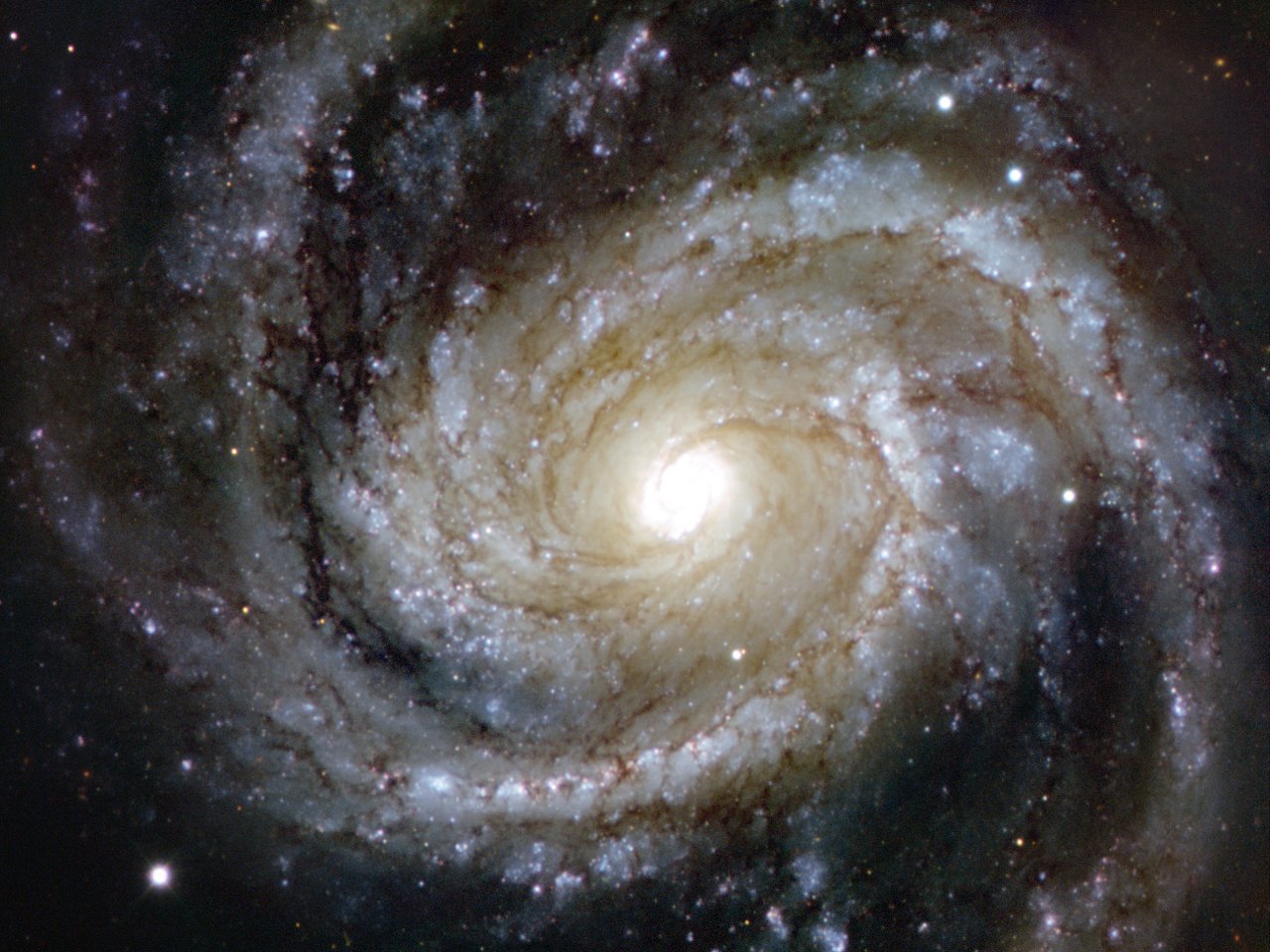


Figure 20.28: M100, a grand-design spiral galaxy, in different wavelengths. Optical (top, left; ESO), ultraviolet-through-near-infrared+H\(\alpha\) composite (top, right; ESO), mid-infrared showing cool and hot dust (bottom, left; NASA/JPL-Caltech), and carbon-monoxide \(J = 2 \rightarrow 1\) line emission (bottom, right; ALMA: [ESO/NAOJ/NRAO] and NRAO/AUI/NSF, B. Saxton). Note that the images are not aligned, especially the bottom-left one.
At the other end of the spiral spectrum are flocculent spirals: spiral structure characterized by a disordered appearance manifesting itself mainly as many fragmented arms without a clear global pattern. An example of a flocculent spiral is NGC 4414, shown in Figure 20.29.
|
|
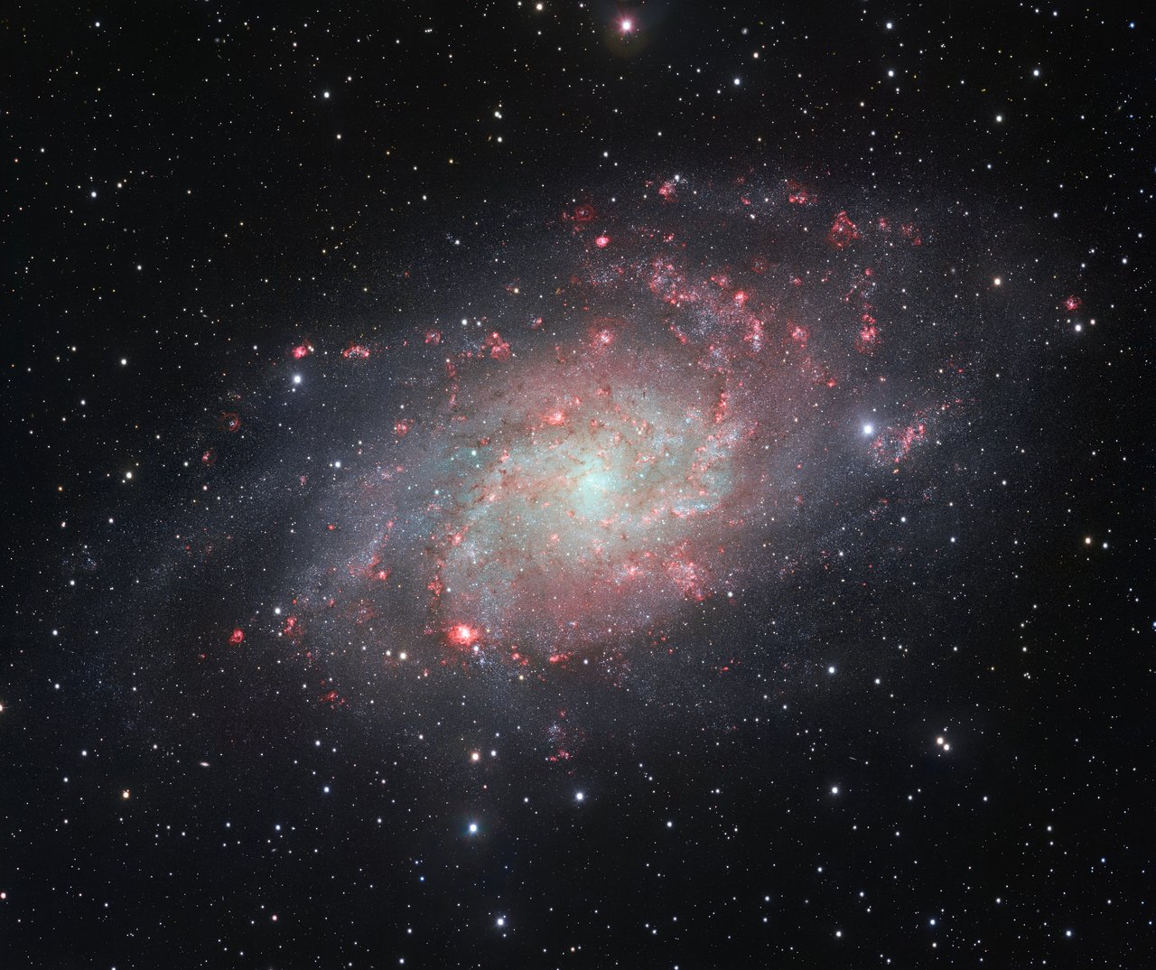

Figure 20.29: M33, an intermediate spiral galaxy (ESO) and NGC 4414, a flocculent spiral (The Hubble Heritage Team/AURA/STScI/NASA).
While spiral structure in grand-design spirals is a global feature, in flocculent spirals it appears to be a local feature and it is, thus, likely that the driving mechanism behind the spiral structure is different.
A range of sub-types can be defined within the class of grand-design spirals based on exactly how global and well-defined the spiral pattern is. The quintessential grand-design spiral has two sharply-defined, symmetric arms extending from the center (or from the ends of the bar as for NGC 1300 in Figure 1.3) all the way to the outskirts of the galaxy. M100 shown in Figure 20.28 is a great example of this. But many galaxies have a global spiral pattern that is less well defined than this and they can be designated as intermediate spiral structure. M101 in Figure 2.1 is an example of this, as is M33 (the Triangulum galaxy) shown in Figure 20.29. In these intermediate spirals, a global pattern can be clearly distinguished, but it does not necessarily extend over the entire face of the galaxy or it can appear irregular in the inner or outer regions.
Elmegreen & Elmegreen (1982) discuss the relative fractions of grand-design versus flocculent galaxies and classify spiral structure into twelve sub-types ranging from chaotically-flocculent to grand grand-design. Among unbarred isolated galaxies, they find that \(\approx 30\%\) of spirals are grand-design, but this fraction rises to \(\gtrsim 70\%\) when considering galaxies in groups, galaxies in a binary pair, or barred galaxies (with weak or strong bars). All but a few percent of grand-design spirals either live in a binary or group, or are barred. Among grand-design spirals, less than half have the quintessential grand-design, with most having intermediate spiral structure. These results indicate that external perturbations from companions or driving by the bar are likely crucial to creating the most striking grand-design patterns that we observe.
Because of our vantage point inside the Milky Way, determining the global appearance of the Milky Way’s spiral structure is difficult. Because the Milky Way was known to be a flat disk, it was suspected to be a spiral nebula, but it was only in the 1950s that observations of young, massive stars (Morgan et al. 1952) and of 21cm neutral-hydrogen emission (van de Hulst et al. 1954; see Figure 20.30) unmistakenly demonstrated that the Milky Way has spiral structure. However, even now the overall structure of the Milky Way’s spiral pattern remains unclear. The best tracers nowadays are high-mass star-forming regions that act as masers—lasers in the microwave spectrum—because their high-intensity radio emission allows their parallaxes, and thus three-dimensional positions in the Galaxy, to be measured precisely using very long baseline interferometry (Reid & Honma 2014). The locations of five spiral arms that can be traced in this way are shown in the right panel of Figure 20.30.
|
|

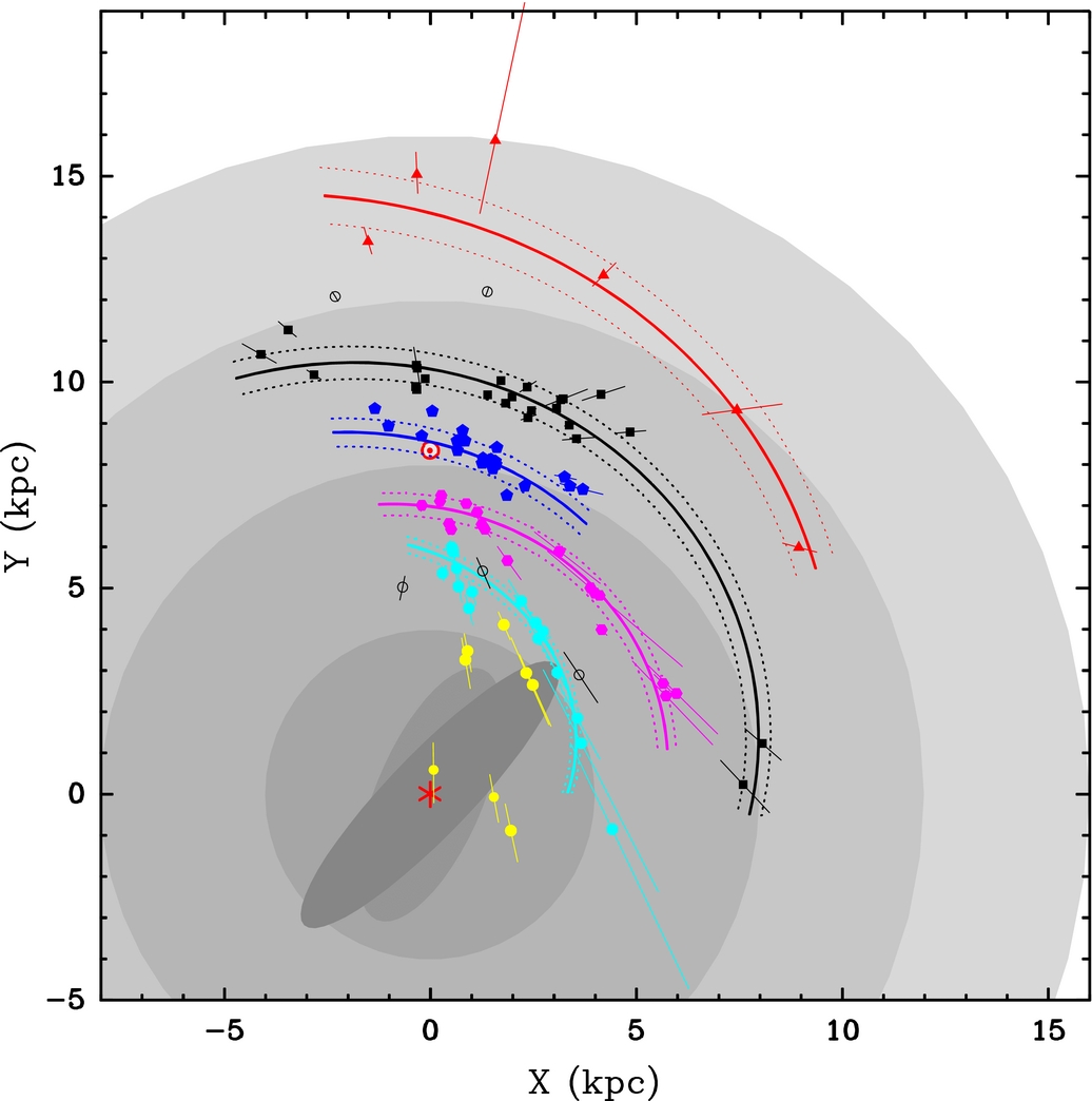
Figure 20.30: Spiral structure in the Milky Way, traced by neutral hydrogen (left; Oort et al. 1958) and high-mass star-forming regions (right; Reid et al. 2014).
The position of the Sun is indicated by the \(\odot\) symbol at \(X=0\). We see that the Sun is located inside a spiral arm, the Local arm, which is believed to be a minor spiral arm. Because we still lack a clear global view of the Milky Way’s spiral structure, we cannot definitively determine whether it is flocculent or not, but the disordered appearance of the nearby spiral structure implies that at most the Milky Way is an intermediate spiral and perhaps a flocculent one, but definitely not a quintessential grand-design spiral.
As Figure 20.28 above shows, grand-design spiral structure manifests itself in almost any galactic component, including the old stellar populations traced by the near- and mid-infrared emission in the top-right and bottom-left panels, the younger stellar populations traced by the optical and ultraviolet emission in the top-left panel, the star-forming gas traced by H\(\alpha\) emission in the top-right and by carbon-monoxide emission in the millimeter range in the bottom-right panel, and dust emission seen in the mid-infrared in the bottom-left image. Figure 20.30 of neutral-hydrogen emission in the Milky Way shows that neutral hydrogen also has spiral structure, which is also seen in external galaxies. A galaxy’s magnetic field also follows the spiral pattern in grand-design spirals (e.g., Fletcher et al. 2011). This again indicates that spiral structure in grand-design spirals is a global phenomenon that involves all of the baryonic components of the galaxy.
We denote spiral patterns as trailing if they trail the rotation of the galaxy—that is, going outwards along a spiral arm one rotates opposite the direction of galactic rotation—and leading otherwise. Determining whether or not an observed pattern is trailing or leading is non-trivial, because while we can observe the rotation of the galaxy using line-of-sight velocities (see Chapter 8.1) , whether or not a spiral pattern is trailing or leading is degenerate with which side of the galaxy is tilted towards us (Slipher 1917). This degeneracy can be broken by determining the tilt of the galaxy, which can be achieved by using the fact that galactic disks are dusty and the near-side of the disk therefore extinguishes more background radiation from spheroidal distributions, e.g., the bulge or the globular-cluster system. When the degeneracy can be broken, all spirals are found to be trailing (Slipher 1917; Hubble 1943; de Vaucouleurs 1958). The exception are a few percent of objects that are largely in interacting pairs (Pasha 1985) and the leading nature is therefore likely a transient response to an external perturbation. NGC 4622 is a rare example of a galaxy with leading spiral arms that has no obvious companion (Buta et al. 2003). Thus, essentially all spiral arms are trailing, as expected from the shearing induced by differential rotation and from the mechanism of swing amplification.
As we already saw in Chapter 18.3, one of the most important geometrical properties of a spiral pattern is its pitch angle. The pitch angle is the angle between the tangents to a spiral and a circle through the same point, as illustrated in the left panel of Figure 20.31.
[61]:
### Pitch angle plot
pitch= 20.*u.deg
ro= 0.2
phi= numpy.linspace(90.,450.,1001)*u.deg
def radius_func(phi,ro=ro,pitch=pitch):
    return ro*numpy.exp(numpy.tan(pitch)*phi.to_value(u.rad))
radii= radius_func(phi)
figure(figsize=(10,5))
subplot(1,2,1)
x,y= radii*numpy.cos(phi), radii*numpy.sin(phi)
plot(x,y,color='tab:blue')
x,y= radii*numpy.cos(phi+180.*u.deg), radii*numpy.sin(phi+180.*u.deg)
plot(x,y,color='tab:blue')
# Pitch angle illustration
def illustrate_pitch_angle(circle_radius=0.75,Ot=None,tangent_offset=1.,
                           plot_circle=True,plot_perp=True,
                           label_angle=True,
                           spiral_color='tab:blue',
                           angle_offset=2.):
    if plot_circle:
        gca().add_patch(Circle((0., 0.), circle_radius,color='0.5',fill=False))
    if Ot is None:
        phi_intersect= numpy.log(circle_radius/ro)/numpy.tan(pitch)*u.rad
        spiral_slope= -1./numpy.tan(phi_intersect-pitch)
    else:
        phi_intersect= numpy.log(circle_radius/ro)/numpy.tan(pitch)*u.rad\
                        +Ot/circle_radius-Ot/radii[0]
        dphi_intersect= 1e-8*u.rad
        dR_intersect= optimize.brentq(
            lambda R: R-radius_func(phi_intersect+dphi_intersect-Ot/R+Ot/radii[0],
                                    ro=ro,pitch=pitch),
            circle_radius,circle_radius+0.1
        )
        spiral_slope= (
            (dR_intersect*numpy.sin(phi_intersect+dphi_intersect)
             -circle_radius*numpy.sin(phi_intersect))/
            (dR_intersect*numpy.cos(phi_intersect+dphi_intersect)
             -circle_radius*numpy.cos(phi_intersect)))
    x_intersect= circle_radius*numpy.cos(phi_intersect)
    y_intersect=circle_radius*numpy.sin(phi_intersect)
    line_circ_perp= plot(
        [x_intersect,x_intersect+tangent_offset],
        [y_intersect,-1./numpy.tan(phi_intersect)*tangent_offset+y_intersect],
        color='0.5',ls='--'
    )[0]
    if plot_perp:
        line_origin= plot([0.,x_intersect],[0.,y_intersect,],
                     color='0.5',ls='--')[0]
    line_spir_perp= plot([x_intersect,x_intersect+tangent_offset],
                         [y_intersect,spiral_slope*tangent_offset+y_intersect],
                         color=spiral_color,ls='--')[0]
    def angle_plot(line1,line2,offset=1,color='k',origin=(0, 0),linestyle='-',
                   len_x_axis=1,len_y_axis=1):
        # Draw angle arc between two lines
        # Edited from https://stackoverflow.com/a/25228427 and
        # https://gist.github.com/battlecook/0c0bdb7097ec7c8fa160e342b1bf51ef
        from matplotlib.patches import Arc
        # Angle between line1 and x-axis
        l1xy= line1.get_xydata()
        slope1= (l1xy[1][1]-l1xy[0][1])/float(l1xy[1][0]-l1xy[0][0])
        angle1= numpy.degrees(numpy.arctan(slope1))
        # Angle between line2 and x-axis
        l2xy= line2.get_xydata()
        slope2= (l2xy[1][1]-l2xy[0][1])/float(l2xy[1][0]-l2xy[0][0])
        angle2= numpy.degrees(numpy.arctan(slope2))
        # Angle between them
        theta1= numpy.amin([angle1,angle2])
        theta2= numpy.amax([angle1,angle2])
        angle= theta2-theta1
        return Arc(origin,len_x_axis*offset,len_y_axis*offset,
                   angle=0,theta1=theta1,theta2=theta2,
                   color=color,linestyle=linestyle)
    gca().add_patch(angle_plot(line_circ_perp,line_spir_perp,
                               angle_offset,origin=[x_intersect,y_intersect]))
    if label_angle:
        galpy_plot.text(-0.3,-1.5,r'$\alpha$',
                        ha='center',va='center',fontsize=18.)
    if plot_perp:
        gca().add_patch(angle_plot(line_circ_perp,line_origin,
                                   0.8,origin=[x_intersect,y_intersect],
                       linestyle='--',color='0.5'))
        galpy_plot.text(-0.1,-0.5,r'$90^\circ$',
                        ha='center',va='center',fontsize=18.,color='0.5')
illustrate_pitch_angle()
xlim(-1.8,1.8)
ylim(-1.8,1.8)
gca().set_aspect('equal')
gca().axis('off')
annotate(r'$\mathrm{pitch\ angle}\ \alpha$',
         (0.5, .95),
         xycoords="axes fraction",
         horizontalalignment="center",
         verticalalignment="top",fontsize=18.)
### Winding problem plot
from scipy import optimize
pitch= 20.*u.deg
ro= 0.2
phi= numpy.linspace(90.,450.,1001)*u.deg
def radius_func(phi,ro=ro,pitch=pitch):
    return ro*numpy.exp(numpy.tan(pitch)*phi.to_value(u.rad))
radii= radius_func(phi)
subplot(1,2,2)
x,y= radii*numpy.cos(phi), radii*numpy.sin(phi)
plot(x,y,color='tab:blue',ls='--')
illustrate_pitch_angle(plot_circle=False,plot_perp=False,label_angle=False)
Ot= -0.75*numpy.pi*u.rad
x= radii*numpy.cos(phi+Ot/radii-Ot/radii[0])
y= radii*numpy.sin(phi+Ot/radii-Ot/radii[0])
plot(x,y,color='tab:pink',lw=2.)
illustrate_pitch_angle(circle_radius=0.75,Ot=Ot,
                       tangent_offset=-1.,
                       plot_circle=False,plot_perp=False,
                       label_angle=False,
                       angle_offset=-1.25,
                       spiral_color='tab:pink')
xlim(-1.8,1.8)
ylim(-1.8,1.8)
gca().set_aspect('equal')
gca().axis('off')
galpy_plot.text(-1.,-1.6,r'$t = 0$',fontsize=18.,color='tab:blue')
galpy_plot.text(0.,1.3,r'$t = T_\phi/2$',fontsize=18.,color='tab:pink')
tight_layout();

Figure 20.31: The pitch angle of a spiral pattern (left) and the winding problem (right).
The pitch angle \(\alpha\) can vary with radius, but grand-design spiral structure is typically well-characterized by a single pitch angle across the galaxy. Because the pitch angle is the quantitative measure of how tightly wound a spiral pattern is, pitch angle varies systematically across the Hubble sequence from Sa to Sd galaxies. Sa-type galaxies have pitch angles \(\alpha \lesssim 10^\circ\), Sb galaxies have \(\alpha \approx 10^\circ\), and Sc galaxies have \(\alpha \approx 15^\circ\), but with a few degree of dispersion within each type (Kennicutt 1981).
Characterizing the strength of spiral arms is usually done using a Fourier decomposition of the light profile as (e.g., Rix & Zaritsky 1995; Yu & Ho 2020): \({I(R,\phi)/ I_0(R)} = 1 + \sum_{m=1}^{\infty}{A_m(R)\,\cos\left(m\phi-m\phi_m[R]\right)}\), where \(I_0(R)\) is the azimuthally-averaged surface density, and \(A_m(R)\) and \(\phi_m(R)\) describe the amplitude and phase of the \(m\)-th Fourier component. Two-armed spirals are dominated by the contribution from the \(A_2(R)\) term, but because strong spirals are not purely sinuisoidal, they also have significant \(A_4(R)\) contributions. The typical value of \(A_2\) in the mid-optical-to-mid-infrared is \(A_2 \approx 0.15\), but very strong spirals have \(A_2 \gtrsim 0.5\). Spirals are \(\approx 25\%\) stronger in blue optical wavelengths (Yu & Ho 2018). Thus, spirals are a weaker relative perturbation than bars and thus typically have a smaller effect on the orbits of stars and gas in a galaxy.
Finally, spiral structure in galaxies is not static, but rotates as the galaxy rotates. Despite early claims of direct proper motion measurements of spiral rotation (van Maanen 1916), determining the angular rotation rate of spiral arms is much more difficult than measuring the bar’s pattern speed. In particular, it is not at all a priori clear that spiral structure rotates with a single pattern speed \(\Omega_p\). If spiral structure results from the shearing by differential rotation of overdensities or through the swing-amplification mechanism, then we would expect the pattern speed to vary with radius to reflect the shear. However, if spiral structure is a long-lived density wave (a possibility that we will discuss below), then it may be characterized by a well-defined single pattern speed. Regardless, observationally one has to assume that the pattern speed may vary with radius.
The Tremaine-Weinberg method of Equation (20.65) that we discussed in the context of bars makes no assumption about the shape of the rotating pattern, so if spiral arms have a well-defined single pattern speed, the Tremaine-Weinberg method applies. If the pattern speed varies with radius, the Tremaine-Weinberg method can be adapted to include radial variations (Merrifield et al. 2006). This has allowed the pattern speeds and their radial variation of a small number of galaxies to be determined (Meidt et al. 2009). Using a more model-dependent method, it is also possible to model observed gas flows in spiral galaxies by dynamical modeling of the axisymmetric background plus spiral arms (e.g., Kranz et al. 2003). While observational determinations of pattern speeds are scant, a few general conclusions have emerged: (i) while some galaxies have a well-defined single pattern speed (e.g., M101; Meidt et al. 2009), others have significant radial variations and (b) in barred galaxies, the spiral pattern speed is usually significantly smaller than the bar’s pattern speed, indicating that bars and spirals are not typically directly associated with each other, although they certainly dynamically interact.
20.3.2. The dynamics of spiral structure
Theories of spiral structure roughly fall in two classes: long-lived—a single pattern existing for many dynamical times—and transient—patterns that only persist for one or a few dynamical times. As we will see below, long-lived spiral structure has to take the form of a density wave and, thus, has to be a long-lived normal mode of the galactic disk—a natural oscillation of the system like an organ’s overtones. Transient spirals are less constrained by the dynamical structure of the disk. They can take the form of simple shearing material arms (see below) or they can be the short-lived response to an internal or external perturbation (e.g., Figure 20.6). As we will see in this and the next sections, transient spiral structure overall seems to provide a better explanation of a wide variety of observations. However, unlike the long-lived density-wave picture, transient spiral structure does not naturally explain why we see clear spiral structure in all disk galaxies aside from lenticular galaxies. If spiral structure is transient, it needs to be constantly regenerated and this is not easy to achieve.
We can make some headway into understanding spiral structure using a few simple dynamical considerations. Due to the differential rotation that characterizes galactic disks, the most obvious explanation for spiral structure is that it results from large-scale density perturbations shearing into trailing spirals at a rate set by the galaxy’s rotational frequency \(\Omega(R) = v_c(R)/R\). This type of spiral structure is known as material arms, because the arms consist of material that remains in the arm at all times. However, this explanation immediately runs into what is known as the winding problem (Prendergast & Burbidge 1960; Oort 1962): material arms would quickly wind up into much tighter patterns than observed. How fast would they wind up? We can estimate this by positing a spiral pattern and calculating how fast it would wind up given a typical rotation curve. Extending Equation (20.1) to non-axisymmetric perturbations, we can write a spiral perturbation to the surface density as \begin{equation}\label{eq-secevol-spiral-perturbation-density} \Sigma_s(R,\phi,t) = \Sigma_s(R,t)\,e^{i\,[m\phi+f(R,t)]}\,, \end{equation} where \(\Sigma_s(R,t)\) is again a slowly-varying function of radius that represents the amplitude of the pattern and the spiral pattern is set by the argument of the exponential, which contains the shape function \(f(R,t)\) and the number of arms \(m\). The crest of the spiral wave is then given by the locus where the argument of the exponential equals an integer multiple of \(2\pi i\): \(m\phi+f(R,t) = 2\,n\,\pi\,,\ n \in \mathbb{Z}\). The pitch angle \(\alpha\) is then given by \begin{equation}\label{eq-intevol-spiral-pitch-as-k} \cot\alpha = \left|R\,{\partial \phi \over \partial R}\right| = \left|{R\over m}\,{\partial f(R,t) \over \partial R}\right| = \left|{k\,R\over m}\right|\,, \end{equation} where we have again defined the wave number \(k = \partial f / \partial R\). For example, for the oft-used logarithmic spiral rotating at a constant pattern speed, \(f(R,t) = -m\,\cot \alpha\,\ln R -m\,\Omega_p\,t\).
Assuming now that the spiral arm is a material arm with each radial section of the arm on a circular orbit around the galaxy, the wave crest is defined by \(m\phi-m\Omega(R)\,t+f(R) = 2\,n\,\pi\,,\ n \in \mathbb{Z}\) and the pitch angle is therefore \begin{equation}\label{eq-intevol-spiral-windingt} \cot\alpha = \left|{R\over m}\,\left({\mathrm{d} \Omega \over \mathrm{d} R}\,t-{\partial f(R) \over \partial R}\right)\right| = \left|2A\,t+{k\,R \over m}\right|\,, \end{equation} where \(A\) is the Oort constant \(A\) from Equation (8.34). For a flat rotation curve, \(2A = \Omega\), so the time dependence can also be written as \(2\pi\,t/T_\phi\), where \(T_\phi\) is the orbital period. Thus, even in the extreme case where the original pattern has \(\alpha_0 = 90^\circ\), the pitch angle becomes \(\alpha \approx 9^\circ\) after a single orbital period and keeps decreasing rapidly as time goes on. For a more realistic initial pitch angle of \(\alpha_0 = 20^\circ\), we have after half an orbital period that \(\alpha \approx 10^\circ\) and after one orbital period that \(\alpha \approx 6^\circ\). The winding in this \(\alpha_0 = 20^\circ\) case is illustrated in the right panel of Figure 20.31, which displays an initial logarithmic material spiral arm (dashed) and the wound-up version after half an orbital period (solid), with pitch angles indicated at the same \(R\). The winding problem demonstrates that if spiral structure consists of material arms, then it cannot be a long-lived structure because all of the observed patterns have \(\alpha \gtrsim 10^\circ\) and would thus have to be \(\lesssim\) one dynamical time old.
For spiral structure to be a long-lived, quasi-static phenomenon in light of the winding problem, spiral structure needs to be a density wave. In this case, spiral arms are a propagating density enhancement in the disk that stars and gas move through as they orbit the galaxy in such a way as to sustain a long-lived spiral pattern (Lindblad 1963; Lin & Shu 1964). We will have much more to say about this in Section 20.3.4 below. But a basic limitation on this view of spiral structure comes from what is known as the anti-spiral theorem (Prendergast 1967; Lynden-Bell & Ostriker 1967). A general statement of the theorem is that because the basic equations of Newtonian dynamics are time-reversible, steady trailing-spiral solutions to the equations describing a galactic disk must be accompanied by steady leading-spiral solutions (obtained by instantaneously flipping the velocities in the trailing solution). A rigorous version of the anti-spiral theorem was proven for fluid disks by Lynden-Bell & Ostriker (1967) and was influential as a criticism of density-wave theory even though it was not entirely clear how the anti-spiral theorem applies to stellar disks. The main implication of the anti-spiral theorem is that spiral structure cannot simply be explained as the natural response of galactic disks to perturbations. Internally in stars, for example, stochastic perturbations excite the star’s normal modes, which we can observe through brightness observations in the fields of helio- and asteroseismology. For disk galaxies, however, if normal spiral modes even exist, we would have to explain why only the trailing modes are excited. This explanation could involve the initial conditions or situations in which the dynamics is not time-reversible, which is the case at the location of the Lindblad resonances (Equation 20.42). Shu (1970) demonstrated that the anti-spiral theorem only holds away from the Lindblad resonances in a stellar disk.
An important observational fact about spiral structure is that grand-design spirals almost always have two arms. It turns out that the dynamical structure of galactic disks is such that they are ideally suited to supporting two-armed spiral structure. The basic insight goes back to Lindblad (1956) who noticed that the rotation curves of many galaxies are such that the combination \(\Omega-\kappa/2\) of the rotational and epicycle frequencies is almost constant over a significant radial range (see, e.g., Figure 20.27). In a frame rotating with a pattern speed \(\Omega_p = \Omega-\kappa/2\), orbits close after two radial oscillations in the epicycle approximation, which we illustrate using the Sun’s orbit over twenty periods (\(\approx\) the age of the Sun) in the left panel of Figure 20.32.
[62]:
from galpy.potential import MWPotential2014, omegac, epifreq
from galpy.orbit import Orbit
o= Orbit()
Tp= 2.*numpy.pi/o.Op(pot=MWPotential2014)
ts= numpy.linspace(0.,20.*Tp,1001)
o.integrate(ts,MWPotential2014)
Op= omegac(MWPotential2014,o.rguiding(),ro=8.,vo=220.,quantity=False)\
    -epifreq(MWPotential2014,o.rguiding(),ro=8.,vo=220.,quantity=False)/2.
fig, ax = subplots(1,2,figsize=(10,5))
sca(ax[0])
o.plot(d1=f'R*cos(phi-{Op}*t)',d2=f'R*sin(phi-{Op}*t)',
       xlabel=r'$x= R\,\cos(\phi-\Omega_p\,t)\,(\mathrm{kpc})$',
       ylabel=r'$y= R\,\sin(\phi-\Omega_p\,t)\,(\mathrm{kpc})$',
       gcf=True,
       label=r'$\Omega_p = \Omega-\kappa/2$')
gca().set_aspect('equal')
legend(frameon=False,fontsize=18.)
sca(ax[1])
from matplotlib.patches import Ellipse
axis_ratio= 8./9.16 # ~that of the Sun's orbit above
radii= numpy.linspace(0.25,3.8,25)
angles= numpy.linspace(50.,-200.,len(radii))
for ii, (radius,angle) in enumerate(zip(radii,angles)):
    ax[1].add_patch(Ellipse((0,0),
                            2*radius,2*radius*axis_ratio,
                            angle=angle,
                            fill=False,color='tab:blue'))
    ax[1].set_xlim(-3.95,3.95)
    ax[1].set_ylim(3.95,-3.95)
    ax[1].set_aspect('equal')
    axis('off');

Figure 20.32: Kinematic density waves. Left panel: the orbit of the Sun in a rotating frame with \(\Omega_p = \Omega-\kappa/2\) in which it approximately closes. Right panel: the creation of a two-armed spiral pattern by orbital crowding in a rotating frame where all orbits approximately close as ellipses.
We see that, because the epicycle approximation is not exact, the Sun’s orbit only approximately closes, but it remains close to a single ellipse for the entire duration of the orbit integration. Now, because \(\Omega-\kappa/2\) is approximately the same over a wide range of radii, we can choose a single pattern speed \(\Omega_p \approx \langle\Omega-\kappa/2\rangle\) and the orbits of the vast majority of disk stars with orbits not much more eccentric than the Sun’s will approximately close in the rotating frame of this pattern speed. By nesting and slightly twisting the major axis as a function of radius, we can then create two-armed spiral patterns that are static in the rotating frame and, thus, rotate with constant pattern speed in the inertial frame (Kalnajs 1973). For ellipses with the approximate axis ratio of the Sun’s orbit in the left panel of Figure 20.32, an example of this is shown in the right panel of the same figure. The density waves created in this manner are purely kinematic density waves resulting from a clever arrangement of orbits in an axisymmetric potential. The fact that \(\Omega-\kappa/2\) is not exactly constant with radius leads again to a winding problem, because the evolution of the pitch angle in Equation (20.84) now becomes \begin{equation}\label{eq-intevol-spiral-windingt-kinematic} \cot\alpha = \left|R\,\left({\mathrm{d} \left[\Omega - \kappa/2\right] \over \mathrm{d} R}\,t+{k\over m}\right)\right| \,. \end{equation} Because \(\mathrm{d}|\Omega - \kappa/2|/\mathrm{d}R \ll \mathrm{d}\Omega/\mathrm{d}R\), this winding up is slower than the original winding problem. For example, for the Milky Way, \(\mathrm{d} (\Omega-\kappa/2)/\mathrm{d}R \approx -0.75\,\mathrm{km\,s}^{-1}\,\mathrm{kpc}^{-2}\); at \(R = 8\,\mathrm{kpc}\) then, \(\mathrm{d} \cot \alpha / \mathrm{d} t \approx -6\,\mathrm{km\,s}^{-1}\,\mathrm{kpc}^{-1} \approx -\Omega/5\), so analogous to the discussion following Equation (20.84), the pattern winds up in \(\approx 5\) dynamical times. While this is longer than we found in the material-arm winding problem, it is still only \(\approx 1\,\mathrm{Gyr}\) for a galaxy like the Milky Way.
Thus, the kinematic-density-wave picture suffers from a similar, though less severe, winding problem as the material-arm picture. But the kinematic-density-wave picture lacks self-gravity entirely and, thus, the real take-away is that the dynamical structure of disk galaxies is such that orbits can easily kinematically arrange themselves into two-armed spiral patterns that remain coherent for long enough that the self-gravity of the pattern can enhance and sustain the pattern for long times. Thus, disk galaxies kinematically prefer two-armed spiral structure and this likely explains the prevalence of two-armed spirals in nature.
For any spiral pattern that is comprised of one or multiple density waves with constant pattern speed, the Lindblad resonances from Equation (20.42) are where orbits are most strongly affected by the spiral potential. We will see in Section 20.3.3 below that this has profound implications for the effect of spiral structure on its galaxy. In addition to the in-plane Lindblad resonances from Equation (20.42), an analogous set of vertical Lindblad resonances exists where the rotational frequency \(\Omega_p - \Omega\) in the rotating frame equals the vertical frequency \(\nu/m\) \begin{equation}\label{eq-intevol-lindblad-vertical} \nu = \pm m\,(\Omega_p - \Omega)\,. \end{equation} Thus, vertical Lindblad resonances are locations where stars oscillate vertically exactly \(m\) times in every rotational period. Because stars at a vertical Lindblad resonance encounter the spiral pattern during the same phase of their vertical orbit each time, vertical Lindblad resonances are the locations where spiral structure most strongly affects the vertical structure of the disk (similar to how the vertical Lindblad resonance of a bar can give rise to bar thickening; see Section 20.2.4 above). Because galactic disks are thin, we always have that \(\nu/\kappa \gg 1\). This implies that the vertical Lindblad resonances are located much further from corotation than the in-plane Lindblad resonances. However, as we discussed in Section 20.1.2, non-axisymmetric perturbations can only propagate between the (planar) Lindblad resonances, so any grand density-wave spiral pattern—whether transient or long-lived—only exists between the (planar) Lindblad resonances. At the location of the vertical Lindblad resonances then, spiral structure does not exist in situ and any effect from the spiral originates far away. Thus, spiral structure has only a minimal impact on the vertical structure of galactic disks. The reason this argument does not hold for galactic bars is that bars are so strong that they change the structure of the galaxy where they reside such that \(\nu/\kappa \approx 1\) and the vertical and planar Lindblad resonances are much closer together.
20.3.3. The effect of spiral structure on its galaxy
Spiral structure can have a profound effect on the structure of disks, but exactly what and how big the effect of spirals is depends on their nature. We will see that steady density-wave spiral structure with a well-defined pattern speed causes few long-term changes to the stellar and gaseous distribution, but transient spiral structure, especially if made up of material arms, can have a much larger effect.
We saw in Section 20.3.1 above that spiral arms in most galaxies are a \(\approx 15\%\) surface-density enhancement. As such, their effect on the disk can be well understood using linear perturbation analysis of the kind that we performed in Sections 20.1.2 and 20.2.3. In those sections, we saw that the effect of small non-axisymmetric perturbations on the velocities (e.g., Equation 20.41) and orbits (e.g., Equation 20.79) of stars and gas are small, except at the Lindblad resonances from Equation (20.42). Thus, large changes to the orbits of individual stars and to the stellar distribution function as a whole only occur at the Lindblad resonances (Lynden-Bell & Kalnajs 1972).
20.3.3.1. Orbits in spiral potentials
To illustrate this point, we can consider the orbit of the Sun in a two-armed spiral model for the Milky Way. To model spiral structure in the Milky Way, we use the analytical model from Cox & Gomez (2002) for the specific case of a two-armed spiral pattern with a pitch angle of \(15^\circ\), a pattern speed of \(2\Omega_0/3\) where \(\Omega_0 = 27.5\,\mathrm{km\,s}^{-1}\,\mathrm{kpc}^{-1}\) is the rotational frequency at the Sun, and an amplitude such that the spiral is a \(\approx 15\%\) surface-density enhancement at the radius of the Sun. We then integrate the orbit of the Sun while slowly growing the spiral structure over \(\approx 10\) spiral periods, keeping the spiral amplitude constant for \(\approx 10\) spiral periods, and letting the spiral decay over another \(\approx 10\) spiral periods. Figure 20.33 then shows the orbit of the Sun before spiral structure forms, during the constant-spiral-amplitude phase, and after the spiral structure has fully decayed.
[63]:
from galpy.potential import (MWPotential2014,
                             SpiralArmsPotential,
                             DehnenSmoothWrapperPotential,
                             vcirc)
from galpy.orbit import Orbit
sp= SpiralArmsPotential(N=2,amp=0.75,phi_ref=25.*u.deg,alpha=15.*u.deg,omega=2./3.)
def integrate_orbit_through_spiral(orb,
                                   dt_start=100.,dt_grow=100.,
                                   dt_on=100.,dt_decay=100.,nt=3001):
    adiabatic_sp= DehnenSmoothWrapperPotential(
        pot=DehnenSmoothWrapperPotential(
            pot=sp,tform=dt_start,tsteady=dt_grow),
        tform=dt_start+dt_grow+dt_on,tsteady=dt_decay,decay=True)
    t_prespiral= numpy.linspace(0.,dt_start,nt)
    t_grow= numpy.linspace(dt_start,dt_start+dt_grow,nt)
    t_on= numpy.linspace(dt_start+dt_grow,dt_start+dt_grow+dt_on,nt)
    t_decay= numpy.linspace(dt_start+dt_grow+dt_on,
                            dt_start+dt_grow+dt_on+dt_decay,
                            nt)
    t_postspiral= numpy.linspace(dt_start+dt_grow+dt_on+dt_decay,
                                 dt_start+dt_grow+dt_on+dt_decay+dt_start,
                                 nt)
    o_prespiral= orb() # copy
    o_prespiral.integrate(t_prespiral,MWPotential2014)
    o_grow= o_prespiral(t_prespiral[-1])
    o_grow.integrate(t_grow,MWPotential2014+adiabatic_sp)
    o_on= o_grow(t_grow[-1])
    o_on.integrate(t_on,MWPotential2014+adiabatic_sp)
    o_decay= o_on(t_on[-1])
    o_decay.integrate(t_decay,MWPotential2014+adiabatic_sp)
    o_postspiral= o_decay(t_decay[-1])
    o_postspiral.integrate(t_postspiral,MWPotential2014)
    return (o_prespiral,o_grow,o_on,o_decay,o_postspiral)
orb= Orbit()
o_prespiral,o_grow,o_on,o_decay,o_postspiral= integrate_orbit_through_spiral(orb)
fig, ax= subplots(
            nrows=2,ncols=3,sharex='col',sharey=False,
            figsize=(10,5),
            gridspec_kw={'height_ratios':[1,2],'hspace':0.04,'wspace':0.05}
        )
xrange= [-10.95,10.95]
yrange= xrange
zrange=[-0.2,0.2]
sca(ax[0,0])
o_prespiral.plot(d1='x',d2='z',gcf=True,
                 xrange=xrange,yrange=zrange,color='tab:blue')
gca().get_xaxis().get_label().set_visible(False)
annotate(r'$t < \mathrm{spiral}$',
         (0.5, 1.2),
         xycoords="axes fraction",
         horizontalalignment="center",
         verticalalignment="top",fontsize=18.)
sca(ax[1,0])
o_prespiral.plot(d1='x',d2='y',gcf=True,
                 xrange=xrange,yrange=yrange,color='tab:blue')
gca().set_aspect('equal')
sca(ax[0,1])
o_on.plot(d1='x',d2='z',gcf=True,
          xrange=xrange,yrange=zrange,color='tab:orange')
gca().get_xaxis().get_label().set_visible(False)
gca().get_yaxis().get_label().set_visible(False)
gca().yaxis.set_major_formatter(NullFormatter())
annotate(r'$t \sim \mathrm{spiral}$',
         (0.5, 1.2),
         xycoords="axes fraction",
         horizontalalignment="center",
         verticalalignment="top",fontsize=18.)
sca(ax[1,1])
o_on.plot(d1='x',d2='y',gcf=True,
          xrange=xrange,yrange=yrange,color='tab:orange')
gca().get_yaxis().get_label().set_visible(False)
gca().yaxis.set_major_formatter(NullFormatter())
gca().set_aspect('equal')
sca(ax[0,2])
o_postspiral.plot(d1='x',d2='z',gcf=True,zorder=10,
                  xrange=xrange,yrange=zrange,color='tab:green')
gca().get_xaxis().get_label().set_visible(False)
gca().get_yaxis().get_label().set_visible(False)
gca().yaxis.set_major_formatter(NullFormatter())
annotate(r'$t > \mathrm{spiral}$',
         (0.5, 1.2),
         xycoords="axes fraction",
         horizontalalignment="center",
         verticalalignment="top",fontsize=18.)
sca(ax[1,2])
o_postspiral.plot(d1='x',d2='y',gcf=True,zorder=0,
                  xrange=xrange,yrange=yrange,color='tab:green')
gca().get_yaxis().get_label().set_visible(False)
gca().yaxis.set_major_formatter(NullFormatter())
gca().set_aspect('equal')
tight_layout();

Figure 20.33: The Sun’s orbit before, during, and after a slowly-grown spiral.
We see that the orbit of the Sun under the influence of the spiral pattern is slightly more eccentric while keeping the same vertical extent (as expected from the argument at the end of the previous section). Overall, the effect of this spiral structure on the orbit of the Sun is small. After the spiral pattern has slowly decayed away, the orbit of the Sun returns to a very similar orbit as before the growth of spiral structure. For this pattern speed, we have that \(R_\mathrm{ILR} \approx 1.36\,\mathrm{kpc}\), \(R_\mathrm{CR} \approx 11.5\,\mathrm{kpc}\), and \(R_\mathrm{OLR} \approx 18\,\mathrm{kpc}\). Thus, the Sun at \(R \approx 8\,\mathrm{kpc}\) is far away from all resonances and the effect of this slowly-evolved spiral pattern is, therefore, small.
To more clearly illustrate that orbits only feel significant effects from steady spirals very close to the Lindblad resonances, we show the long-term effect of the same spiral pattern as above for circular orbits near the inner Lindblad resonance. The top row of Figure 20.34 displays the initial circular orbit before the slow growth of the spiral pattern and the final orbit after the spiral pattern has slowly decayed.
[64]:
from galpy.potential import lindbladR
from galpy.orbit import Orbit
Rs= [lindbladR(MWPotential2014,sp.OmegaP(),m=2)*0.9,
     lindbladR(MWPotential2014,sp.OmegaP(),m=2),
     lindbladR(MWPotential2014,sp.OmegaP(),m=2)*1.1]
fig, ax= subplots(
            nrows=2,ncols=3,sharex=False,sharey=False,
            figsize=(10,6.666),
            gridspec_kw={'hspace':0.04,'wspace': 0.04}
        )
for ii,R in enumerate(Rs):
    # Slow
    orb= Orbit([R,0.,vcirc(MWPotential2014,R),0.,0.,0.],ro=8.,vo=220.)
    o_prespiral,o_grow,o_on,o_decay,o_postspiral= \
        integrate_orbit_through_spiral(orb,dt_start=20.)
    sca(ax[0,ii])
    o_prespiral.plot(d1='x',d2='y',gcf=True,zorder=10,lw=2.,
                     xrange=[-2.22,2.22],yrange=[-2.22,2.22])
    o_postspiral.plot(d1='x',d2='y',overplot=True,zorder=8)
    gca().set_aspect('equal')
    gca().get_xaxis().get_label().set_visible(False)
    gca().xaxis.set_major_formatter(NullFormatter())
    if ii > 0:
        gca().get_yaxis().get_label().set_visible(False)
        gca().yaxis.set_major_formatter(NullFormatter())
    else:
        galpy_plot.text(r'$\mathrm{Slow}$',top_left=True,fontsize=18.)
    if ii != 1:
        galpy_plot.text(rf'$R = {R/Rs[1]:.1f}\,R_{{\mathrm{{ILR}}}}$',top_right=True,fontsize=18.)
    else:
        galpy_plot.text(rf'$R = R_{{\mathrm{{ILR}}}}$',top_right=True,fontsize=18.)
    # Fast
    orb= Orbit([R,0.,vcirc(MWPotential2014,R),0.,0.,0.],ro=8.,vo=220.)
    o_prespiral,o_grow,o_on,o_decay,o_postspiral= \
        integrate_orbit_through_spiral(orb,dt_grow=5.,dt_decay=5.,dt_start=30.)
    sca(ax[1,ii])
    o_prespiral.plot(d1='x',d2='y',gcf=True,zorder=10,lw=2.,
                     xrange=[-2.2,2.2],yrange=[-2.2,2.2])
    o_postspiral.plot(d1='x',d2='y',overplot=True,zorder=5)
    gca().set_aspect('equal')
    if ii > 0:
        gca().get_yaxis().get_label().set_visible(False)
        gca().yaxis.set_major_formatter(NullFormatter())
    else:
        galpy_plot.text(r'$\mathrm{Fast}$',top_left=True,fontsize=18.)
tight_layout();

Figure 20.34: The effect of a spiral perturbation on circular orbits near the inner Lindblad resonance.
We see that the effect of the spiral perturbation is large only at the location of the resonance and that even just inside and outside the resonance, the effect is substantially smaller. The effect at the outer Lindblad resonance is similar, although even at the resonance the effect of the spiral is smaller. Thus, the long-term effects of a steady spiral perturbation are concentrated at the Lindblad resonances.
When spiral structure comes and goes more rapidly, as in models of transient spiral structure, the Lindblad resonances are broadened and a wider range of orbits near the Lindblad resonances are significantly affected. For example, growing and decaying the spiral pattern over only about half a spiral period rather than ten, we see that the effects near the inner Lindblad resonance in the bottom row of Figure 20.34 is much larger.
Near the corotation radius, a different behavior occurs. In Figure 20.35, we see the long-term behavior of circular orbits near corotation in the fast-growth, fast-decay spiral model.
[65]:
from galpy.potential import lindbladR
from galpy.orbit import Orbit
Rs= [lindbladR(MWPotential2014,sp.OmegaP(),m='corot')*0.9,
     lindbladR(MWPotential2014,sp.OmegaP(),m='corot'),
     lindbladR(MWPotential2014,sp.OmegaP(),m='corot')*1.1]
fig, ax= subplots(
            nrows=1,ncols=3,sharex=False,sharey=False,
            figsize=(10,3.333),
            gridspec_kw={'hspace':0.125,'wspace': 0.04}
        )
for ii,R in enumerate(Rs):
    orb= Orbit([R,0.,vcirc(MWPotential2014,R),0.,0.,4.*numpy.pi/9.],ro=8.,vo=220.)
    o_prespiral,o_grow,o_on,o_decay,o_postspiral= integrate_orbit_through_spiral(orb,dt_grow=5.,dt_decay=5.)
    sca(ax[ii])
    o_prespiral.plot(d1='x',d2='y',gcf=True,zorder=10,
                     xrange=[-18,18],yrange=[-18,18])
    o_postspiral.plot(d1='x',d2='y',overplot=True)
    if ii != 1:
        galpy_plot.text(rf'$R = {R/Rs[1]:.1f}\,R_{{\mathrm{{CR}}}}$',top_right=True,fontsize=18.)
    else:
        galpy_plot.text(rf'$R = R_{{\mathrm{{CR}}}}$',top_right=True,fontsize=18.)
    gca().set_aspect('equal')
    if ii%3 > 0:
        gca().get_yaxis().get_label().set_visible(False)
        gca().yaxis.set_major_formatter(NullFormatter())
tight_layout();

Figure 20.35: Like the bottom row of Figure 20.34, but for circular orbits just inside, at, and just outside the corotation radius.
We see that at the corotation resonance, orbits sustain long-term effects that persist after the spiral pattern decays away. But rather than orbits becoming non-circular and, thus, more eccentric, circular orbits near corotation are shifted in radius without incurring significant non-circularity.
We can understand the difference in behavior between corotation on the one hand and the Lindblad resonances on the other hand by considering orbits in the frame of the spiral perturbation. Assuming that the spirals rotate with a fixed pattern speed \(\Omega_p\), the Jacobi integral from Equation (19.55) is a conserved quantity. This implies that changes in the specific angular momentum \(L\) of an orbit must be accompanied by changes in the specific energy \(E\) as \begin{equation}\label{eq-intevol-spiral-dEdLfromJacobi} \Delta E = \Omega_p\,\Delta L_z\,. \end{equation} We can use this relation to determine what type of orbit an initially-circular orbit becomes after interacting with the spiral pattern. This is done visually in the so-called Lindblad diagram (Lindblad 1933) shown in Figure 20.36, which shows the location of orbits, in particular circular ones, in the plane of specific energy versus specific angular momentum.
[66]:
from galpy.potential import (MWPotential2014, vcirc,
                             evaluatePotentials, rl, lindbladR)
from matplotlib.patches import FancyArrowPatch
def Ec(L):
    Rc= rl(MWPotential2014,L)
    return evaluatePotentials(MWPotential2014,Rc,0.)+L**2./2./Rc**2.
Ls= numpy.linspace(0.01,2.5,101)
figure(figsize=(6,4))
ymin= -3.49
plot(Ls,[Ec(L) for L in Ls],'k-',lw=2.)
fill_between(Ls,ymin,[Ec(L) for L in Ls],color='gray',zorder=-1)
Omegap= 2./3.
def jacobi_line(Lfid,Efid,Lmin,Lmax,arrowstyle=None,**kwargs):
    if not arrowstyle is None:
        arrow = FancyArrowPatch((Lmin, Omegap*(Lmin-Lfid)+Efid),
                                (Lmax, Omegap*(Lmax-Lfid)+Efid),
                                arrowstyle=arrowstyle,
                                mutation_scale=20,
                                zorder=10)
        gca().add_patch(arrow)
    else:
        plot([Lmin,Lmax],
             [Omegap*(Lmin-Lfid)+Efid,Omegap*(Lmax-Lfid)+Efid],
             **kwargs)
for m in [-2,2,'corot']:
    RLR= lindbladR(MWPotential2014,Omegap,m=m)
    LLR= RLR*vcirc(MWPotential2014,RLR)
    plot([LLR],[Ec(LLR)],'ko',ms=10.)
    jacobi_line(LLR,Ec(LLR),
                LLR-m/2*0.4 if m != 'corot' else LLR+0.4,
                LLR if m != 'corot' else LLR-0.4,
                arrowstyle='<->' if m == 'corot' else '<-')
    annotate(
        rf'$\mathrm{{{"CR" if m == "corot" else ("ILR" if m == 2 else "OLR")}}}$',
        xy=(LLR-0.22,Ec(LLR)+0.22),va='bottom',fontsize=16.
    )
jacobi_line(LLR,Ec(LLR)+0.0,gca().get_xlim()[0],
            0.95*gca().get_xlim()[1],
            ls='--',color='0.5')
annotate(r'$\mathrm{Forbidden}$',(1.2, -2),
         fontsize=16.,
         bbox=dict(edgecolor='none',facecolor='w',alpha=1.))
annotate(r'$\partial E/\partial L =\Omega_p$',(-0.4,-1.5),
         fontsize=16.,rotation=18.)
xlabel(r'$L$')
ylabel(r'$E$')
ylim(ymin,0.6);

Figure 20.36: Lindblad diagram after Sellwood & Binney (2002).
We see that at the inner and outer Lindblad resonances, the line with \(\partial E/\partial L =\Omega_p\) points away from the circular-orbit locus. This means that circular orbits at the Lindblad resonances become eccentric orbits after interacting with spirals. At the corotation radius, however, the line with \(\partial E/\partial L =\Omega_p\) is parallel to the circular-orbit locus, because for circular orbits \(\partial E/\partial L =\Omega\) and corotation is where \(\Omega = \Omega_p\). Therefore, circular orbits at corotation move to circular orbits just inside or outside corotation under the influence of spiral structure—this process is known as churning (Sellwood & Binney 2002). These are exactly the types of behavior that we observed in Figures 20.34 and 20.35. More generally, the close-to-circular orbits that dominate in the disks of galaxies remain close to circular at their guiding-center radius away from any of the resonances, they remain close to circular but move to another radius at corotation, and they become more eccentric at the inner and outer Lindblad resonances.
The way churning proceeds is that orbits near corotation can get trapped in the resonance, orbiting around only a segment of the spiral pattern rather than passing in and out of all spiral arm segments. In the rotating frame where the spiral pattern is static, such orbits librate around part of the pattern rather than performing full rotations around the center. An example of a closed trapped orbit in the Milky-Way spiral model from above is given in Figure 20.37.
[67]:
from galpy.potential import (MWPotential2014,
                             SpiralArmsPotential,
                             NonInertialFrameForce,
                             lindbladR,
                             plotDensities)
from galpy.orbit import Orbit
sp= SpiralArmsPotential(N=2,amp=0.75,
                        phi_ref=10.*u.deg,alpha=15.*u.deg,
                        ro=8.,vo=220.)
Omegap= 2./3.
nip= NonInertialFrameForce(Omega=Omegap)
Rcorot= lindbladR(MWPotential2014,Omegap,m='corot')
Tp= 2.*numpy.pi/Omegap
o= Orbit([Rcorot,0.,0.96-Omegap*Rcorot,0.09725-numpy.pi/2.],ro=8.,vo=220.)
ts= numpy.linspace(0.,200*Tp,10001)
o.integrate(ts,MWPotential2014+sp+nip)
figure(figsize=(5,5))
o.plot(d1='x',d2='y',xrange=[-16.,16.],yrange=[-16.,16.],lw=3.,gcf=True)
gca().set_aspect('equal');
gca().add_artist(Circle((0,0),Rcorot*8.,
                        color='0.2',fill=False,ls='--',lw=2.))
plotDensities(sp,xy=True,log=True,
              rmin=gca().get_xlim()[0]*u.kpc,
              rmax=gca().get_xlim()[1]*u.kpc,nrs=100,
              zmin=gca().get_ylim()[0]*u.kpc,
              zmax=gca().get_ylim()[1]*u.kpc,nzs=100,
              overplot=True,justcontours=True,
              ncontours=26,cntrlw=0.5);

Figure 20.37: Horseshoe orbit near corotation in the rotating frame of a Milky-Way-like spiral potential. The corotation locus is shown as the dashed gray circle.
We see that the orbit librates around the corotation radius. When it is at \(R > R_\mathrm{CR}\), a star on this orbit falls behind the spiral pattern, moving upwards along the outer segment of the orbit. This continues until the star reaches the next spiral crest, which slowly pulls the star towards the center. As the star passes the corotation radius to \(R < R_\mathrm{CR}\), the star starts to move faster than the spiral pattern and moves downwards along the inner segment, again until it reaches the crest of the spiral pattern, which now pulls the star away from the center and the star passes \(R= R_\mathrm{CR}\) again and starts its loop again. This type of orbit is known as a horseshoe orbit, because it resembles a horseshoe in the context of planetary dynamics, where these orbits appear in the rotating frame of two orbiting point masses (see Figure 19.19) .
When we combine horseshoe orbits near corotation with transient spiral structure, we obtain the ability to move close-to-circular orbits from one side of the corotation radius to the other. An example is shown in Figure 20.38. Here we modulate the amplitude of the spiral pattern with a Gaussian: \(\mathrm{amp} \propto \exp\left(-[t-t_0]^2/\sigma_t^2\right)\). This causes the spiral pattern to grow and decay over a typical time scale \(\sigma_t\) and reach its peak at \(t_0\). In each panel, the orbit starts out outside of corotation before the growth of the spiral pattern (blue curves) and ends up inside after it decays (green curves); during the growth and decay of the pattern, the orbit is traced by the thick orange curve. Varying \(\sigma_t\) between \(2.5\,T_p\) and \(7.5\,T_p\), where \(T_p = 2\pi/\Omega_p\) is the spiral period, we see the evolution for example orbits near corotation in Figure 20.38.
[68]:
from galpy.potential import (GaussianAmplitudeWrapperPotential,
                             MWPotential2014,
                             SpiralArmsPotential,
                             NonInertialFrameForce,
                             lindbladR,
                             plotDensities)
from galpy.orbit import Orbit
sp= SpiralArmsPotential(N=2,amp=0.75,
                        phi_ref=10.*u.deg,alpha=15.*u.deg,
                        ro=8.,vo=220.)
Omegap= 2./3.
nip= NonInertialFrameForce(Omega=Omegap)
Rcorot= lindbladR(MWPotential2014,Omegap,m='corot')
Tp= 2.*numpy.pi/Omegap
figure(figsize=(10,5))
for ii,(tsp, o, ton) in enumerate(
    zip(
        [GaussianAmplitudeWrapperPotential(pot=sp,to=40.*Tp,sigma=2.5*Tp),
         GaussianAmplitudeWrapperPotential(pot=sp,to=40.*Tp,sigma=7.5*Tp)],
        [Orbit([Rcorot+0.04,0.,0.95-Omegap*Rcorot,0.09725-numpy.pi/2.],
               ro=8.,vo=220.),
         Orbit([Rcorot+0.04,0.,0.95-Omegap*Rcorot,0.09725-numpy.pi/2.],
               ro=8.,vo=220.)],
        [35.*Tp,30.*Tp]
    )
):
    ts_pre= numpy.linspace(0.,ton,201)
    ts_on= numpy.linspace(ton,80*Tp-ton,201)
    ts_post= numpy.linspace(80*Tp-ton,80*Tp,201)
    o.integrate(ts_pre,MWPotential2014+tsp+nip)
    subplot(1,2,ii+1)
    o.plot(d1='x',d2='y',gcf=True,xrange=[-16.,16.],yrange=[-16.,16.],lw=2.,ls='-')
    o= o(ts_pre[-1])
    o.integrate(ts_on,MWPotential2014+tsp+nip)
    o.plot(d1='x',d2='y',overplot=True,lw=4.,ls='-')
    o= o(ts_on[-1])
    o.integrate(ts_post,MWPotential2014+tsp+nip)
    o.plot(d1='x',d2='y',overplot=True,lw=2.,ls='-')
    gca().set_aspect('equal');
    gca().add_artist(Circle((0,0),Rcorot*8.,
                    color='tab:gray',fill=False,ls='--',lw=2.))
    plotDensities(sp,xy=True,log=True,
              rmin=gca().get_xlim()[0]*u.kpc,
                  rmax=gca().get_xlim()[1]*u.kpc,
                  nrs=100,
              zmin=gca().get_ylim()[0]*u.kpc,
                  zmax=gca().get_ylim()[1]*u.kpc,
                  nzs=100,
              overplot=True,justcontours=True,
                  ncontours=26,cntrlw=0.5)
    if ii > 0:
        gca().get_yaxis().get_label().set_visible(False)
        gca().yaxis.set_major_formatter(NullFormatter())
tight_layout();

Figure 20.38: Churning near corotation using a transient spiral pattern. In the right panel, the growth and decay of the spiral pattern is three times slower than in the left panel.
We see that the spiral pattern is significantly felt for just the right amount of time to move the orbit from the apocenter of its horseshoe orbit to its pericenter. Thus, the effect of the transient spiral is to move the orbit inwards by, in this case, \(1.5\,\mathrm{kpc}\). This is a significant change in radius, similar to the typical epicycle amplitude of stars near the Sun (see Chapter 9.3.2). In the right panel, the spiral perturbation last so long that the orbit performs multiple horseshoe loops. In the example that we have chosen, after the spiral pattern fades, the orbit is still deposited about \(1\,\mathrm{kpc}\) inwards, but as the pattern lasts longer, the chance that the orbit will be left at a radius close to where it started increases and the overall effect of churning on the radial distributions of stars is diminished.
20.3.3.2. The age–velocity-dispersion relation and kinematical heating
Thus, short-lived transient spiral structure significantly affects the orbits of stars near the orbital resonances: transient spirals increase the eccentricity of orbits near the Lindblad resonances and move stars to orbits of similar eccentricity near the corotation radius. These two types of behavior are important to explaining two observational facts about galactic disks and the Milky Way disk in particular:
The velocity dispersion of stars increases with age as \(\sigma \propto t^\beta\), with \(\beta \approx 0.3\) in the radial and rotational directions and \(\beta \approx 0.5\) in the vertical direction;
The chemical distribution of stars indicates a significant amount of radial migration of stars within the disk.
We already saw in Chapter 10.3.1 that the velocity dispersion of stellar populations near the Sun increases with their color (see Figure 10.4). Because color is a proxy for the mean age of the stellar population, this observation is a manifestation of an underlying relation between age and velocity dispersion. After early measurements of this relation by, e.g., Wielen (1974), a definitive determination of this relation for the different components of the velocity vector in the solar neighborhood was performed using data from the Geneva-Copenhagen survey by Nordstrom et al. (2004) and it is shown in the left panel of Figure 20.39.
|
|
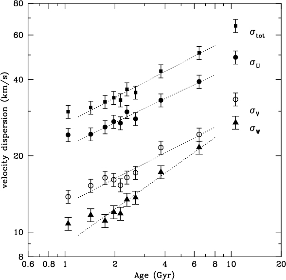

Figure 20.39: Left panel: Velocity dispersion in the radial (U), rotational (V), and vertical (W) directions as a function of age for stars near the Sun (Nordstrom et al. 2004). Right panel: Age–metallicity relation of stars near the Sun from Edvardsson et al. (1993).
We see that the velocity dispersion in all three components increases approximately as a power law \(\sigma \propto t^\beta\), with \(\beta \approx 0.3\) for the radial (\(\sigma_U\)) and rotational (\(\sigma_V\)) components of the velocity, while \(\beta \approx 0.5\) for the vertical component (\(\sigma_W\)). These relations can now be determined using much larger samples of stars extending far away from the solar neighborhood, but the basic power-law exponents for the different components remain the same (e.g., Mackereth et al. 2019). Because \(\sigma_U\) and \(\sigma_V\) have the same power-law exponent, their ratio is independent of age and is \(\sigma_V/\sigma_U \approx 0.63\) (Nordstrom et al. 2004). Because the vertical velocity dispersion increases faster with age than the radial dispersion, their ratio increases with time, from \(\sigma_W/\sigma_U \approx 0.4\) for the youngest age populations to \(\sigma_W/\sigma_U \approx 0.6\) for the older populations. Thus, the shape of the velocity ellipsoid only changes mildly with age, but it does change.
Because stars form in a cold, low-velocity dispersion (\(\sigma \lesssim 10\,\mathrm{km\,s}^{-1}\)) disk at the present age of the Universe and this seems to have been the case for at least the last \(\approx 8\,\mathrm{Gyr}\) (Wisnioski et al. 2015), these age–velocity-dispersion relations are best explained as resulting from kinematical heating, increasing the typical eccentricity of stellar orbits over time through interactions with inhomogeneities in the gravitational potential (Wielen 1977). Various mechanisms can play a role in this heating. While the two-body relaxation times in galaxies are so long that encounters between individual stars do not appreciably change their orbits over the age of the Universe (see Chapter 5.1), Spitzer & Schwarzschild (1951) were the first to suggest that encounters between stars and giant molecular clouds (GMCs) can lead to secular increases in the velocity dispersion with time (see also Spitzer & Schwarzschild 1953). Similarly, if the dark-matter halo consists of massive compact halo objects (MACHOs), such as primordial black holes, then encounters between stars and MACHOs lead to secular increases in the velocity dispersion (Lacey & Ostriker 1985). However, the heating from MACHOs is predicted to be \(\sigma_W \propto \sigma_U \propto t^{0.5}\) with \(\sigma_W/\sigma_U \approx 0.5\), which disagrees with the observed \(\sigma_U \propto t^{0.3}\). Heating by molecular clouds, however, leads to \(\sigma_U \propto t^{0.2}\) (Hanninen & Flynn 2002), also disagreeing with the observations. Finally, Barbanis & Woltjer (1967) suggested that transient spiral structure consisting of episodes lasting a few hundred Myr each can give rise to heating in the \(\sigma_U\) and \(\sigma_V\) dispersions, but as we have seen in this and the previous section, spirals do not significantly perturb the vertical motions of stars and, thus, lead to very little heating in \(\sigma_W\). Because the massive \(M \approx 10^6\,M_\odot\) MACHOs that would be required for significant MACHO heating are strongly disfavored on a variety of grounds (Carr et al. 2021; Banik & Bovy 2021) and heating by orbiting satellites is far too small to explain the velocity dispersions of even intermediate-age stars, only the combination of GMC and spiral heating remains as a plausible explanation for the observed age–velocity-dispersion relation.
To see how spiral structure causes heating, we can study orbits perturbed by weak spiral structure in the same manner as we used for orbits in weak bars in Section 20.2.3. We again work in the rotating frame, now rotating at the spiral pattern speed \(\Omega_p\), and the equations of motion to first order are again given by Equations (20.73). We then consider a tightly-wound spiral potential perturbation in the rotating frame \begin{equation}\label{eq-secevol-spiral-perturbation-potential} \Phi_s(R,\phi) = \Phi_m(R)\,\cos\left[m\phi+f(R)\right]\,, \end{equation} where \(\Phi_m(R)\) represents the slow radial variation of the perturbation and \(k = \mathrm{d} f / \mathrm{d} R\). We have that \(|k| \gg m/R_0\), because the pattern is tightly-wound (see Equation 20.83). This spiral perturbation is related to the surface-density perturbation of Equation (20.82) by Equation (20.4). Equations (20.75) then become \begin{align}\label{eq-intevol-spirals-weak-eom-wphi1m-1} -{\partial \Phi_1 \over \partial R}\Bigg|_{R_0} & = -{\mathrm{d} \Phi_{m} \over \mathrm{d}R}\Bigg|_{R_0}\,\cos\left[m\phi+f(R)\right]+k\,\Phi_m(R)\,\sin\left[m\phi+f(R)\right]\\ & \approx k\,\Phi_m(R)\,\sin\left[m\phi+f(R)\right]\,,\label{eq-intevol-spirals-weak-eom-wphi1m-2}\\ -{\partial \Phi_1 \over \partial \phi}\Bigg|_{R_0} & = m\,\Phi_{m}(R_0) \,\sin\left[m\phi+f(R)\right] \approx 0\,,\label{eq-intevol-spirals-weak-eom-wphi1m-4} \end{align} where in the second line we have used that the radial variation of \(\Phi_m\) is much smaller in magnitude than \(|k\,\Phi_m(R)|\) and in the third line we used the tightly-wound assumption. Keeping the full derivatives for now, we can derive the spiral version of Equation (20.78) under the same assumption that we can use unperturbed quantities in the argument of the sine and cosine \begin{align} & {\mathrm{d}^2 R_1 \over \mathrm{d} \phi_0^2} + R_1\,{\kappa^2_0\over (\Omega_0-\Omega_p)^2} = 2\,{R_0\,\Omega_0\over (\Omega_0-\Omega_p)}\,C+{1\over (\Omega_0-\Omega_p)^2}\,k\,\Phi_m(R)\,\sin\left[m\phi_0+f(R_0)\right]\nonumber\\ & \quad -{1\over (\Omega_0-\Omega_p)^2}\,\left[{\mathrm{d} \Phi_{m} \over \mathrm{d}R}\Bigg|_{R_0}+2{\Omega_0\over (\Omega_0-\Omega_)\,R_0} \,\Phi_{m}(R_0)\right]\,\cos\left[m\phi_0+f(R_0)\right]\label{eq-intevol-spirals-weak-eom-dr1}\,, \end{align} where we have also expanded \(f(R) \approx f(R_0) + k\,R_1\). This is again the equation of motion of a forced harmonic oscillator with the external force consisting now of two sinusoidal components and a constant component (see Appendix B.4.2). The effect of the constant forcing is again to shift the equilibrium value of \(R_1\) by a constant, so we ignore it. The solution of this equation is then \begin{align} & R_1(\phi_0) =A\,\cos\left({\kappa_0\over \Omega_0-\Omega_p}\,\phi_0+\phi_0^0\right) + {1 \over \kappa_0^2-m^2\,(\Omega_0-\Omega_p)^2}\,k\,\Phi_m(R)\,\sin\left[m\phi_0+f(R_0)\right]\nonumber\\ &\quad - {1 \over \kappa_0^2-m^2\,(\Omega_0-\Omega_p)^2}\,\left[{\mathrm{d} \Phi_{m} \over \mathrm{d}R}\Bigg|_{R_0}+2{\Omega_0\over (\Omega_0-\Omega_p)\,R_0} \,\Phi_{m}(R_0)\right]\,\cos\left[m\phi_0+f(R_0)\right]\,.\label{eq-intevol-spirals-weak-eom-r1sol} \end{align} It is clear from this solution that orbits are again significantly perturbed at the Lindblad and corotation resonances, as expected. Like in the equivalent discussion for bar orbits below Equation (20.79), closed orbits are once more given by solutions with \(A=0\) and the equation above shows that the circular orbit in the axisymetric potential at \(R_0\) becomes elliptical with radius \(R_1(\phi_0)\). But this orbit is not heated in the sense that it is still as ordered as it was in the axisymmetric potential. Thus, if a spiral pattern rotates steadily, orbits are not kinematically heated, except perhaps right at the resonances where the perturbation analysis does not hold.
To see how a transient pattern does induce heating, we consider the same perturbation as in Equation (20.88), but we modulate its amplitude using a Gaussian \(f(t) = \exp\left(-t^2/[2\,\sigma_t^2]\right)\). To keep things relatively simple, we use the approximations from Equations (20.90) and (20.91) and Equation (20.92) then becomes \begin{align}\label{eq-intevol-spirals-weak-eom-dr1-transient} & {\mathrm{d}^2 R_1 \over \mathrm{d} t^2} + R_1\,\kappa^2_0 = k\,\Phi_m(R)\,f(t)\,\sin\left[m\phi_{0,0}+m\,(\Omega_0-\Omega_p)t+f(R_0)\right]\,, \end{align} where we additionally ignored the constant forcing and we use Equation (20.71) to turn the \(\phi_0\) and its derivatives into time and its derivatives. The solution of this equation is \begin{align} & R_1(t) = A\,\cos\left({\kappa_0\over \Omega_0-\Omega_p}\,\phi_0+\phi_0^0\right) \\ &\ + {k\,\Phi_m(R) \over \kappa_0}\,\int_{-\infty}^t\mathrm{d}t'\,f(t')\,\sin\left[m\phi_{0,0}+m\,(\Omega_0-\Omega_p)t'+f(R_0)\right]\,\sin\left[\kappa_0\,(t-t')\right]\,.\nonumber \end{align} The closest analog to circular orbits in this transient spiral pattern are the orbits with \(A=0\). For those, the behavior at \(t \gg \sigma_t\) is \begin{align} R_1(t) = & {\sqrt{2\pi}\,\sigma_t\,k\,\Phi_m(R) \over 2\,\kappa_0} \,\Bigg\{\cos\left[\kappa_0\,t-m\phi_{0,0}-f(R_0)\right]\,\exp\left[-\sigma_t^2\,(m[\Omega_0-\Omega_p]+\kappa_0)^2/2\right]\nonumber\\&\quad -\cos\left[\kappa_0\,t+m\phi_{0,0}+f(R_0)\right]\,\exp\left[-\sigma_t^2\,(m[\Omega_0-\Omega_p]-\kappa_0)^2/2\right]\Bigg\}\,. \end{align} This expression demonstrates that after the transient spiral pattern has faded away, the radius near the Lindblad resonances oscillates and has, thus, become more eccentric due to the interaction with the spiral pattern. When \(\sigma_t \gg 1/\Omega_0\), the oscillation is only significant very close to the Lindblad resonances, because the oscillations are exponentially suppressed as \(\exp\left[-\sigma_t^2\,(m[\Omega_0-\Omega_p]\pm\kappa_0)^2/2\right]\). But if \(\sigma_t \approx 1/\Omega_0\), then radial oscillations and, thus, heating, are induced over a significant fraction of the disk. When \(\sigma_t \ll 1/\Omega_0\), the factor of \(\sigma_t\) in front of the curly braces suppresses the response. Thus, transient spirals with a duration of order the dynamical time are most efficient at heating galactic disks. The induced radial oscillation has an amplitude \(\Delta R \approx (2\pi)^{1/2}\,\sigma_t\,k\,\Phi_m(R) /(4\,\kappa_0)\). Using Equation (20.4), we can write this in terms of the surface-density perturbation \begin{equation} \Delta R \approx {(2\pi)^{3/2}\,G\,\Sigma_m(R) \over 4\,\kappa_0\,\Omega_0}\,\sigma_t\,\Omega_0\,. \end{equation} We can turn this into a typical velocity dispersion using the relation between the epicycle amplitude and the velocity dispersion from Chapter 9.3.2 and write it in terms of the spiral overdensity \(\Sigma_m/\Sigma_0\) and the velocity dispersion of the disk using the Toomre \(Q\) parameter from Equation (20.29): \begin{equation}\label{eq-intevol-spiral-heating} \sqrt{\langle v^2_R\rangle} \approx {(2\pi)^{3/2}\,\sigma_R \over 13.44\,\sqrt{2}\,Q}\,{\kappa_0\over \Omega_0}\,{\Sigma_m\over \Sigma_0}\,\sigma_t\,\Omega_0\approx {\sigma_R\over 7}\,{1 \over Q}\,{\kappa_0\over \Omega_0}\,{6\,\Sigma_m\over \Sigma_0}\,(\sigma_t\,\Omega_0)\,, \end{equation} where all of the factors following the \(\sigma_R/7\) factor in the second expression are approximately one for a typical spiral disk. Thus, a single transient spiral episode with a duration \(\sigma_t \approx 1/\Omega_0\) causes the velocity dispersion to increase by about one seventh of the typical velocity dispersion of the disk.
Multiple episodes of transient spiral structure then cause steady heating of the disk. For \(\sigma_t \approx 1/\Omega\), the pattern rises and falls over the course of about a dynamical time \(t_\mathrm{dyn} = 2\pi/\Omega_0\), so the disk can easily squeeze in \(t_\mathrm{disk}/t_\mathrm{dyn}\) episodes of transient spiral structure, where \(t_\mathrm{disk}\) is the age of the disk, assuming spiral structure is efficiently regenerated—as it must be to explain the ubiquitousness of spiral structure. Because the induced epicycle phases are uncorrelated between spiral episodes, the epicycle amplitude performs a random walk and the velocity dispersion therefore increases with the number of spiral episodes \(N_s\) as \(\sqrt{N_s}\). Equation (20.98) for multiple episodes then becomes \begin{equation}\label{eq-intevol-spiral-heating-multi} \sqrt{\langle v^2_R\rangle} \approx \sigma_R\,{\sqrt{N_s}\over 7}\,{1 \over Q}\,{\kappa_0\over \Omega_0}\,{6\,\Sigma_m\over \Sigma_0}\,(\sigma_t\,\Omega_0)\,. \end{equation} Near the Sun, \(t_\mathrm{disk}/t_\mathrm{dyn} \approx 50\), so it is plausible that \(N_s \approx 50\) and then \(\sqrt{\langle v^2_R\rangle} \approx \sigma_R\). Thus, spiral heating can on its own explain the radial velocity dispersion of old stars in the disk. Assuming that spiral episodes occur evenly-spaced in time, the velocity dispersion increases \(\propto \sqrt{N_s} = \sqrt{t}\). Numerical simulations demonstrate that actually \(\sigma \propto t^{0.3}\), because spiral heating starts to saturate once the epicycle amplitude becomes similar to the radial spiral spacing (e.g., De Simone et al. 2004), while still being able to explain the entire radial velocity dispersion in the disk. Thus, both the amplitude and the time-dependence of the radial velocity dispersion can be explained by transient spiral heating. Because spirals cannot efficiently heat in the vertical direction, they cannot on their own explain the vertical age–velocity-dispersion relation, but it turns out that GMCs efficiently re-distribute the in-plane heating to include the vertical velocity as well (Binney & Lacey 1988). Thus, the combination of spiral heating with GMC redistribution of this heating to the vertical velocity can explain the age–velocity dispersion observed in all three velocity components in the Milky Way disk.
One issue with the above picture is that the heating caused by transient spiral structure quickly causes the Toomre \(Q\) parameter of a purely-stellar disk to rise to \(Q \gtrsim 2\) (Sellwood & Carlberg 1984). At this \(Q\), the disk becomes unresponsive to perturbations (see Figure 20.10), such that it no longer supports transient spiral structure and heating saturates. However, even a small amount of gas that remains kinematically cold due to its ability to cool radiatively (see Chapter 19.3.1) is enough to keep \(Q\approx 1.5\) where the disk remains highly responsive to perturbations and can support many episodes of transient spiral structure (this allowed us to keep \(Q\) constant in Equation 20.99). This is then also the likely explanation for why lenticular disk galaxies lack spiral structure: they are devoid of gas and young stars and, thus, unable to keep \(Q\) small enough to sustain spiral structure.
20.3.3.3. The age–metallicity relation and spiral churning
We discussed the chemical evolution of galaxies in Chapter 11 in terms of simple single-zone models. While the evolution of the overall metallicity and the abundance ratios varies strongly with the rates of gas inflow and outflow, with the adopted star-formation histories and the chemical yields and time evolution of different enrichment processes, all of these single-zone models predict that there is a well-defined and tight relation between stellar age and stellar metallicity that results from long-lived stars recording the homogeneous abundance of the interstellar medium at the time of their birth. However, direct observations of the age–metallicity relation in the solar neighborhood and beyond demonstrate that there is essentially no correlation between age and metallicity for stars with ages \(\lesssim 8\,\mathrm{Gyr}\) and perhaps even for older ages. This was first clearly seen in a sample of 189 stars by Edvardsson et al. (1993) and has since been confirmed with much larger data sets (e.g., Haywood et al. 2013). We show the original observation from Edvardsson et al. (1993) in the right panel of Figure 20.39. We see that the metallicity as a function of age is essentially flat at \([\mathrm{Fe/H}] \approx 0\) for the last 8 Gyr (\(\log_{10} 8 \approx 0.9\)) and that it has a wide scatter.
The observed age–metallicity relation is unexpected in simple models of chemical evolution. For example, in the delayed accreting box model from Chapter 11.3.4 with parameters set to quickly or slowly reach \([\mathrm{Fe/H}] \approx 0\) today, we would expect the age–metallicity relations shown in Figure 20.40.
[69]:
def feh_accretingbox(t,p_Fe_Ia=0.001,p_Fe_II=0.0011,
                     tau_Ia=0.4,tau_Ia_2=3.3,mindt=0.05,
                     tau_star=1.,solar_Fe=7.5,
                     eta=2.25,r=0.4):
    tau_dep= tau_star/(1.+eta-r)
    tau_tilde= 1./(1./tau_Ia-1./tau_dep)
    dt= t-mindt
    out= p_Fe_Ia/(1.+eta-r)\
        *(1.-numpy.exp(-dt/tau_dep)
          +tau_tilde/tau_dep*(numpy.exp(-dt/tau_Ia)
                              -numpy.exp(-dt/tau_dep)))
    # Second exponential Ia component
    if not tau_Ia_2 is None:
        out/= 2.
        tau_tilde= 1./(1./tau_Ia_2-1./tau_dep)
        out+= p_Fe_Ia/2./(1.+eta-r)\
        *(1.-numpy.exp(-dt/tau_dep)
          +tau_tilde/tau_dep*(numpy.exp(-dt/tau_Ia_2)
                              -numpy.exp(-dt/tau_dep)))
    out[t<mindt]= 0.
    # Add CCSN contribution
    out+= p_Fe_II/(1.+eta-r)*(1.-numpy.exp(-t/tau_dep))
    # Convert to [Fe/H]
    logZFe_solar= -2.90+solar_Fe-7.50
    return numpy.log10(out)-logZFe_solar
ts= numpy.geomspace(1e-3,10.,201)
figure(figsize=(6,4))
plot(10.-ts,feh_accretingbox(ts,eta=1.),
     label=r'$\tau_* = \phantom{0}1\,\mathrm{Gyr},\ \eta = 1$')
plot(10.-ts,feh_accretingbox(ts,tau_star=10.,eta=.5),
     label=r'$\tau_* = 10\,\mathrm{Gyr},\ \eta = 0.5$')
xlabel(r'$\mathrm{Age}\,(\mathrm{Gyr})$')
ylabel(r'$[\mathrm{Fe/H}]$')
ylim(-1.2,0.5)
legend(frameon=False,fontsize=18.);

Figure 20.40: Age–metallicity relations in the delayed accreting box model from Chapter 11.3.4.
We see that if enrichment is slow, a clear anti-correlation between age and \([\mathrm{Fe/H}]\) should exist, but if enrichment is fast the relation can be flat. However, in the absence of processes that move stars across a large range of Galactocentric radii, we expect the scatter around these relations to be \(\approx 0.1\), much smaller than is observed. This number comes from the effect of epicyclic motions: In Chapter 9.3.2, we saw that the typical epicycle amplitude of old stars near the Sun is \(\approx 1.4\,\mathrm{kpc}\), which combined with a metallicity gradient of \(\approx -0.085\,\mathrm{kpc}^{-1}\) for stars near the Sun (Hayden et al. 2014) gives rise to a \(\approx 0.1\) scatter in the metallicity at a given age. The fact that many intermediate-age stars near the Sun have metallicities as low as \([\mathrm{Fe/H}] \approx -0.5\) and as high as \([\mathrm{Fe/H}] \approx 0.3\) means, using the same metallicity gradient, that they originate from Galactocentric radii ranging from \(\approx 4.5\,\mathrm{kpc}\) to \(\approx 14\,\mathrm{kpc}\). This encompasses the region starting from the end of the bar to the outermost disk!
Because the present-day interstellar medium has little scatter in its metallicity at a given Galactocentric radius (e.g., Luck & Lambert 2011) and because there is little scatter in the relation between age and the relative abundance of alpha elements (O, Mg, Si, etc.) to iron, it appears that the metallicity of the interstellar medium at any given radius has always been homogeneous. Thus, the large scatter in the stellar age–metallicity relation must have been induced after stars were born in a process generally referred to as radial migration. Churning due to transient spiral structure is able to move stars over large distances and, thus, introduce this large amount of scatter in the age–metallicity relation. But because churning only occurs at the corotation radius, it requires different episodes of transient spiral structure to have different pattern speeds with a resultant wide range of corotation radii such that stars can travel large radial distances by hopping from one corotation resonance to the next. An example of this hopping for the orbit shown in the left panel of Figure 20.38 is displayed in Figure 20.41.
[70]:
from galpy.potential import (GaussianAmplitudeWrapperPotential,
                             MWPotential2014,
                             SpiralArmsPotential,
                             lindbladR,
                             plotDensities)
from galpy.orbit import Orbit
sp1= SpiralArmsPotential(N=2,amp=0.75,
                         phi_ref=10.*u.deg,alpha=15.*u.deg,
                         omega=2./3.,
                         ro=8.,vo=220.)
sp2= SpiralArmsPotential(N=2,amp=0.75,
                         phi_ref=20.*u.deg,alpha=15.*u.deg,
                         omega=2./3.+0.1,
                         ro=8.,vo=220.)
sp3= SpiralArmsPotential(N=2,amp=0.75,
                         phi_ref=20.*u.deg,alpha=15.*u.deg,
                         omega=2./3.+0.225,
                         ro=8.,vo=220.)
Rcorot= lindbladR(MWPotential2014,2./3.,m='corot')
Tp1= 2.*numpy.pi/(2./3.)
sp_pot= GaussianAmplitudeWrapperPotential(pot=sp1,to=40.*Tp1,sigma=2.5*Tp1)\
    +GaussianAmplitudeWrapperPotential(pot=sp2,to=60.*Tp1,sigma=2.5*Tp1)\
    +GaussianAmplitudeWrapperPotential(pot=sp3,to=80.*Tp1,sigma=2.5*Tp1)
o= Orbit([1.51395362,0.03122257,0.95385984,2.1385553],ro=8.,vo=220.)
ts_pre= numpy.linspace(25.*Tp1,35.*Tp1,1001)
ts_on1= numpy.linspace(35.*Tp1,45.*Tp1,1001)
ts_post1= numpy.linspace(45*Tp1,55*Tp1,1001)
ts_on2= numpy.linspace(55.*Tp1,65*Tp1,1001)
ts_post2= numpy.linspace(65*Tp1,75*Tp1,1001)
ts_on3= numpy.linspace(75.*Tp1,85*Tp1,1001)
ts_post3= numpy.linspace(85*Tp1,95*Tp1,1001)
o.integrate(ts_pre,MWPotential2014+sp_pot)
figure(figsize=(6,6))
o.plot(d1='x',d2='y',gcf=True,
       xrange=[-13.,13.],yrange=[-13.,13.],lw=2.,
       label=rf'$\langle R \rangle = {numpy.mean(o.R(ts_pre,quantity=False)):.1f}\,\mathrm{{kpc}}$')
o= o(ts_pre[-1])
o.integrate(ts_on1,MWPotential2014+sp_pot)
#o.plot(d1='x',d2='y',overplot=True,lw=.5)
o= o(ts_on1[-1])
o.integrate(ts_post1,MWPotential2014+sp_pot)
o.plot(d1='x',d2='y',overplot=True,lw=2.,
      label=rf'$\langle R \rangle = {numpy.mean(o.R(ts_post1,quantity=False)):.1f}\,\mathrm{{kpc}}$')
o= o(ts_post1[-1])
o.integrate(ts_on2,MWPotential2014+sp_pot)
#o.plot(d1='x',d2='y',overplot=True,lw=2.)
o= o(ts_on2[-1])
o.integrate(ts_post2,MWPotential2014+sp_pot)
o.plot(d1='x',d2='y',overplot=True,lw=2.,
      label=rf'$\langle R \rangle = {numpy.mean(o.R(ts_post2,quantity=False)):.1f}\,\mathrm{{kpc}}$')
o= o(ts_post2[-1])
o.integrate(ts_on3,MWPotential2014+sp_pot)
#o.plot(d1='x',d2='y',overplot=True,lw=2.)
o= o(ts_on3[-1])
o.integrate(ts_post3,MWPotential2014+sp_pot)
o.plot(d1='x',d2='y',overplot=True,lw=2.,
       label=rf'$\langle R \rangle = {numpy.mean(o.R(ts_post3,quantity=False)):.1f}\,\mathrm{{kpc}}$')
gca().set_aspect('equal')
legend(frameon=False,fontsize=17.);

Figure 20.41: An orbit hopping from an initial close-to-circular orbit at \(R \approx 12\,\mathrm{kpc}\) to a final close-to-circular orbit at \(R \approx 8\,\mathrm{kpc}\) using the corotation resonances of three episodes of spiral structure. Only segments of the orbit before, in-between, and after the spiral episodes are shown.
The orbit starts out with \(R \approx 12\,\mathrm{kpc}\) and has a small eccentricity \(e \approx 0.03\). Three episodes of spiral structure then move the orbit steadily inwards while maintaining its eccentricity by churning around the three corotation radii located roughly in between each of the orbit segments shown. We have chosen the spiral parameters such that the orbit steadily moves inwards. In reality, the pattern speeds are likely such that the next corotation resonance can be inwards or outwards from the current orbit, so the orbit can be carried inwards or outwards for any given episode of spiral structure with similar chance. Or an episode’s corotation radius may be so distant that no churning occurs for this particular orbit during the episode. Thus, like heating, churning by a sequence of transient spiral episodes is a random walk, but now in the value of the guiding-center radius rather than the epicycle amplitude.
To better see churning in action, the following orbit animation displays the orbit above as it goes through the three episodes of spiral structure. It was generated using:
[89]:
o= Orbit([1.51395362,0.03122257,0.95385984,2.1385553],ro=8.,vo=220.)
o.integrate(numpy.linspace(25*Tp1,95*Tp1,3001),MWPotential2014+sp_pot)
o.animate(d1='x',d2='y',width=500.,height=500.); # Remove ; to display the animation
The situation of transient spiral episodes nicely separated in time in the example above is highly idealized, but \(N\)-body simulations of galactic disks demonstrate that the orbit hopping through churning at corotation resonances happens similarly in realistic simulations (e.g., Roskar et al. 2008). Four example orbits that nicely illustrate the random-walk nature of the orbit hopping in these realistic simulations are shown in Figure 20.42.
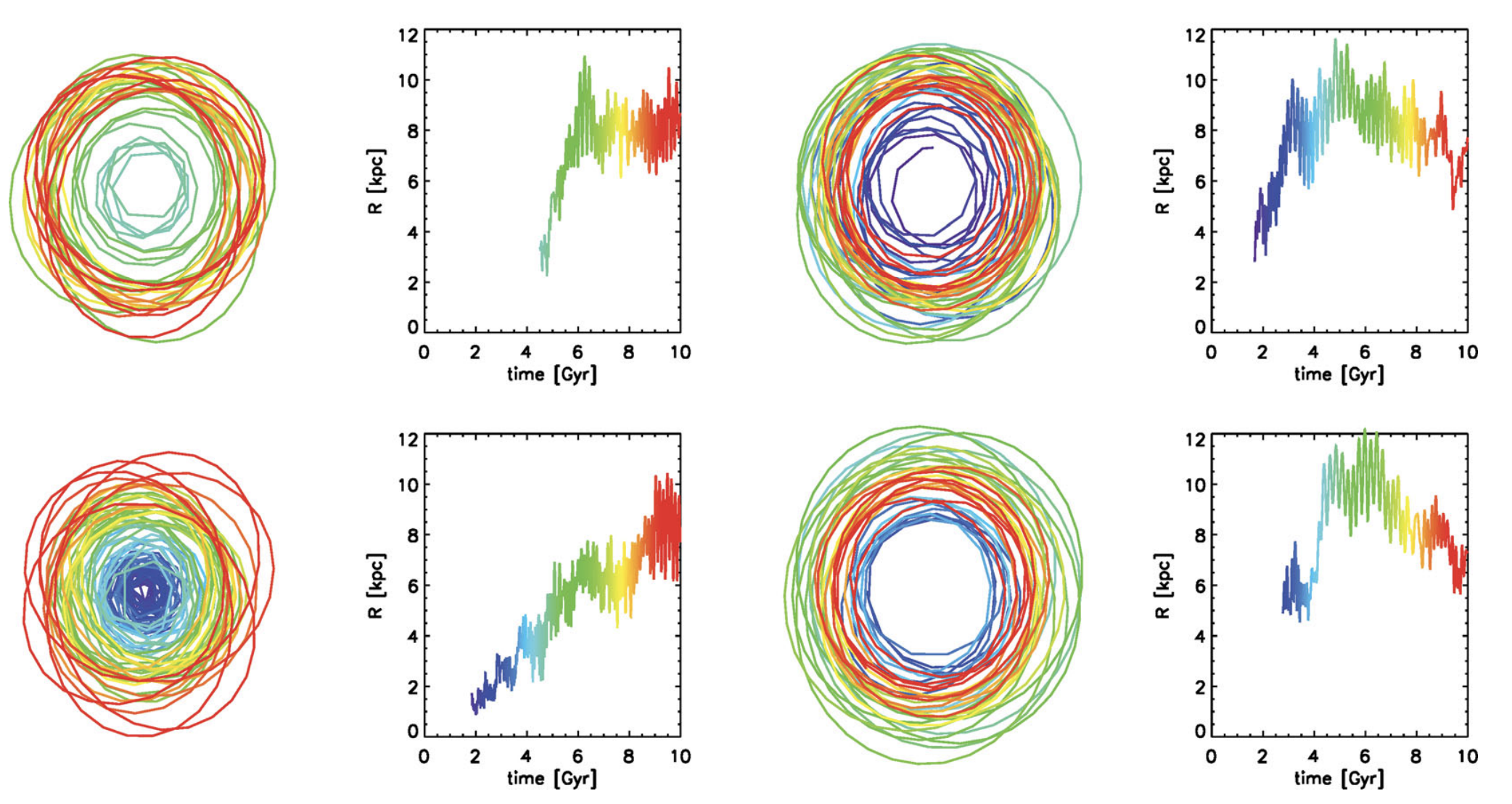
Figure 20.42: Orbit hopping at the corotation resonances of many episodes of transient spiral structure in a hydrodynamical \(N\)-body simulation from Roskar et al. (2012).
We see that the orbit hopping is, as expected, more stochastic than in the idealized example of Figure 20.41, but that overall the orbit hopping is qualitatively similar and that orbits can move across many kpc in the course of a few Gyr. Simulations clearly demonstrate that churning is a process that leaves the overall angular momentum distribution unchanged, as churning essentially leads to orbits near corotation swapping place.
Aside from its effect on the age–metallicity relation of galactic disks, radial migration also strongly affects the outer structure of disks, because the properties of the low number of stars directly forming in a galaxy’s outskirts are easily changed by a small number of stars migrating in from the disk’s inner regions—the same number of stars migrates inwards, where they have less effect because of the higher density of in situ stars. For example, radial migration may fill in a galaxy’s outskirts and lead to breaks in the outer density profile (Roskar et al. 2008). In the Milky Way, radial migration may be the cause of the unexpected positive skew of the metallicity distribution in the outer disk (Hayden et al. 2015), by populating the intrinsic negatively-skewed distribution with enough higher metallicity stars from the inner Milky Way to change the skew from negative to positive.
20.3.3.4. Angular-momentum transport by spiral structure
Thus, we conclude that while the effect of steady spiral perturbations on the structure of a galactic disk are small except very close to the Lindblad resonances, transient spiral structure with episodes lasting \(\mathcal{O}(t_\mathrm{dyn})\) lead to significant heating and churning in the disk. The overall effect of spiral structure is to transport angular momentum outwards (Lynden-Bell & Kalnajs 1972), thus allowing the galaxy to evolve to a lower entropy state as we discussed at the start of this chapter. The net amount of angular momentum transport, however, is small even for transient spiral episodes. This can be seen from the following argument. As we saw in Equation (20.87), specific energy and angular-momentum changes due to a non-axisymmetric perturbation with a fixed pattern speed \(\Omega_p\) are related by \(\Delta E = \Omega_p\,\Delta L_z\). Considering orbits in the \(z=0\) mid-plane, we can decompose the specific energy into the specific energy \(E_c(L_z)\) of a circular orbit with specific angular momentum \(L_z\) and the contribution \(E-E_c(L_z)\) from the orbit’s non-circularity. Quantifying the latter contribution using the radial action \(J_R\) from Chapter 9.4, we can write Equation (20.87) as (Sellwood & Binney 2002) \begin{align}\label{eq-intevol-spiral-dEdLfromJacobi-intermsofJR} \Omega_p\,\Delta L_z& = \Delta E \approx {\partial E \over \partial J_R}\, \Delta J_R + {\partial E \over \partial L_z}\,\Delta L_z = \Omega_R\, \Delta J_R + \Omega_\phi\,\Delta L_z\,, \end{align} where in the final step we have used Equation (3.72) and the fact that \(L_z\) is the azimuthal action \(J_\phi\). Thus, changes to the specific angular momentum are related to changes in the orbit’s circularity (parameterized through \(\Delta J_R\)) as \begin{equation}\label{eq-intevol-spiral-dLz-dJr} \Delta L_z \approx {\Omega_R \over \Omega_p - \Omega_\phi}\,\Delta J_R\,. \end{equation} For close-to-circular orbits, \(\Omega_R = \kappa\) and \(\Omega_\phi = \Omega\), so using Equation (20.41) we can write this also as \(\Delta L_z \approx \pm m\,\Delta J_R\), where \(m=2\) at the Lindblad resonances, \(m=\infty\) at corotation, and \(m \sim O(1) \in \mathbb{R}\) away from the resonances for most of the disk. Now, because even the kinematically-warmest parts of a galactic disk have \(J_R \ll L_z\), we must have that \(\Delta J_R \ll L_z\) and, therefore, \(\Delta L_z \ll L_z\). Thus, specific angular momentum changes caused by spiral structure—whether it is steady or the combined effect of many transient episodes—are small compared to the overall angular-momentum structure of the disk.
20.3.4. Formation and evolution of spiral structure
When it was unclear that all galaxies manifest strong differential rotation, spiral structure was considered to mainly be a phenomenon of the gas and dust in a galaxy that was likely maintained by magnetic fields (e.g., Burbidge 1962; Baade 1963). But by the 1960s it became abundantly clear that differential rotation produces strong shears that leads to the winding problem discussed above, such that spiral structure came to be understood as a dynamical phenomenon. Highly influential in that time (and still!) was the Lin-Shu hypothesis (Lin & Shu 1964) that spiral structure is a quasi-stationary mode in galactic disks (see also Lindblad 1963). This theory naturally accounts for the fact that spiral structure is so ubiquitous in galaxies—if spirals are long-lived, then of course we see them in almost all disk galaxies—but from the outset this theory was beset by problems. We already discussed one of them above, the anti-spiral theorem, which essentially states that we should expect both leading and trailing spirals if we want to explain spiral structure purely in terms of the modes of a galactic disk.
A more serious problem for quasi-stationary spiral structure was uncovered by the discovery of the group velocity of propagating waves in galactic disks (Toomre 1969). In Section 20.1.2 above, we saw that non-axisymmetric perturbations have a dispersion relation given by Equation (20.44) for stellar disks and by Equation (20.45) for gas disks. In stellar disks with \(Q > 1\), waves can propagate between the inner Lindblad resonance and a radius inside coration as well as between a radius outside corotation and the outer Lindblad resonance (see Figure 20.7 where \(|s|=1\) corresponds to the Lindblad resonances and \(s=0\) to corotation). In this region, spiral wave packages propagate at the group velocity, which is proportional to the slope of the lines in the left panel of Figure 20.7 (see the right panel of Figure 20.7 for an illustration of how waves propagate). The dispersion relation implies that quasi-stationary spiral modes of the disk can only exist in the wave-propagation region and to get spiral structure covering most of the disk then requires (i) \(Q \approx 1\) such that the waves can propagate almost to the corotation radius and (ii) \(m=2\) such that the Lindblad resonances are as far away as possible from the corotation radius (remember that corotation is equivalent to \(m=\infty\) in the Lindblad resonance equation 20.42). When \(Q=1\), waves can propagate from the inner Lindblad resonance all the way to corotation and even pass through corotation to travel all the way to the outer Lindblad resonance. However, Figure 20.7 shows that as waves propagate in this way, they get ever more tightly wound, so the quasi-stationary spiral waves are in fact not quasi-stationary, but suffer from a similar winding problem as material spiral arms! Quasi-stationary spiral structure of the Lin-Shu form can then only exist if the structure of the disk is such that the growth and propagation/winding of spiral waves is so slow as to take many dynamical times (Bertin & Lin 1996). However, because the disk has to live so close to \(Q=1\), it is likely unstable to other fast-growing modes that would quickly heat the disk to \(Q \gg 1\), causing spiral structure to cease. Thus, quasi-stationary spiral structure does not appear to be a good model for spiral structure in galaxies.
If spiral structure is transient, the question becomes how it is continuously excited such that we see spiral structure in all gas-rich disk galaxies and such that the smooth kinematical heating from the previous section occurs. It is clear that at least some grand-design spiral structure is tidally excited by companion galaxies. For example, M51 has a massive companion NGC 5195 and the tidal interaction between the two can easily account for all of the observed features of M51’s spiral structure (see Figure 19.2; Toomre & Toomre 1972; Dobbs et al. 2010), including the radial variation of its pattern speed (Meidt et al. 2008). This radial variation of the pattern speed strongly argues against a quasi-stationary spiral model and for a transient response that is in the process of winding up. M81 in Figure 1.3 is another example of this, likely tidally interacting with its companions M82 and NGC 3077 (Yun et al. 1994).
However, not all spiral disks have nearby companions massive enough to excite grand-design spiral structure and spiral structure must therefore also be able to be excited otherwise. Luckily, as we saw in Section 20.1.2 above, realistic galactic disks are highly responsive to perturbations in a way that creates strong spiral structure. Goldreich & Lynden-Bell (1965) and Julian & Toomre (1966) demonstrated that perturbations from a massive orbiting perturber like a giant molecular cloud create strong spiral-shaped perturbations in local patches of the galactic disk through the process of swing amplification. More detailed simulations of this scenario found that the response is stronger than that expected from simple linear theory, due to the non-linear effect of the guiding-center radii of stars becoming correlated in a way that amplifies the response (Toomre & Kalnajs 1991). More recently, D'Onghia et al. (2013) performed global numerical simulations of the response of a galactic disk to massive orbiting molecular clouds and found that they produce long-lived, self-perpetuating spiral responses. The spiral structure created in this way does not have the global coherence of grand-design spiral structure, instead better matching the flocculent type of spiral structure seen in many spirals.
Strong spiral structure also results simply from Poisson noise in the density distribution of stellar disks. Using a set of simulations of galactic disks with \(5\times 10^4\) to \(5 \times 10^8\) particles, Sellwood (2012) demonstrated that spiral structure with an overdensity of \(\delta \approx 20\%\) always forms no matter how smooth the initial distribution of particles is. They found that growth is slow until \(\delta \approx 2\%\) after which non-linear growth quickly increases \(\delta\). Because their simulation with \(5 \times 10^8\) particles is smoother than typical galactic disks, which have a lower effective number of particles due to the massive giant molecular clouds in them, this shows that spiral structure is always expected to occur in relatively cool galactic disks. That non-linear effects commence at \(\delta \approx 2\%\) is likely due to similar correlations in the guiding-center radii of stars as found by Toomre & Kalnajs (1991).
Thus, spiral structure easily emerges in galactic disks with \(1 \lesssim Q \lesssim 2\) as the response to any perturbations grown through the process of swing amplification and helped along by the dynamical structure of galactic disks that allows two-armed spiral structure in particular to emerge over a large fraction of the disk from the non-linear effects of correlations between nearby orbits. This spiral response is transient, lasting \(\mathcal{O}(t_\mathrm{dyn})\), and must therefore be efficiently re-generated to be consistent with the ubiquitousness of spiral structure in observed galactic disks. The nature of transient spirals seen in simulations is still somewhat unclear, with some simulations finding that transient spirals consist of a superposition of a few slowly-evolving modes with fixed pattern speeds (e.g., Quillen et al. 2011; Roskar et al. 2012; Sellwood & Carlberg 2014), while other simulations find transient patterns that wind at the local shearing rate everywhere (such spirals effectively corotate everywhere; Wada et al. 2011; Grand et al. 2012). Regardless of their exact nature, in both of these scenarios strong heating and radial migration occurs that is consistent with the observations and considerations that we discussed in the previous section.
Simulations also show that spiral structure is very effective at regenerating itself perpetually, at least if the disk can remain cool enough through a supply of fresh gas (Sellwood & Carlberg 1984). This regeneration can occur through the non-linear coupling of multiple patterns with different pattern speeds (Tagger et al. 1987), non-linear effects turning leading perturbations into trailing ones that can swing amplify once more (see Section 20.1.2; Fuchs et al. 2005), or by density (D'Onghia et al. 2013) or distribution-function (Sellwood & Lin 1989; Sellwood & Kahn 1991) inhomogeneities acting as new perturbations that grow into a new spiral episode. Thus, many mechanisms exist that plausibly explain the recurrence of spiral structure seen in all modern simulations of disk galaxies. Aside from providing heating and churning mechanisms that can explain the observed age–velocity-dispersion and age–metallicity relations as we saw in the previous section, transient spiral structure also naturally explains the moving groups seen in the velocity distribution of stars near the Sun (Figure 10.9; e.g., De Simone et al. 2004; Bovy & Hogg 2010) and the complex pattern of mean radial-velocity motions in the Milky Way disk observed by Gaia (Kawata et al. 2018; Hunt et al. 2019).
We discussed at the end of Section 20.3.1 how the pattern speeds of bars and spiral structure in the same galaxy are typically different, such that most instances of the ends of the bar lining up with the spiral arms are chance coincidences. However, in strong bars, orbits near the unstable Lagrange points \(L_1\) and \(L_2\) at the ends of the bar (see Figure 20.14) flow away from the bar in spiral-like morphologies (Tsoutsis et al. 2009; Athanassoula et al. 2009). Thus, in some barred galaxies, a direct connection between the bar and spiral structure may exist.

 .
. .
. .
.