← Previous section Next chapter →

11.3. The evolution of abundance ratios

\label{sec-chemev-evolaburatios}

In the classical models of galactic chemical evolution that we have considered so far, where all recycling is instantaneous and there is a single, time-independent yield, all elements evolve with time in the same way. The only difference between elements is their yield, because the mass of, say, iron yielded by a stellar population is lower than the mass of, for example, oxygen. The abundance \(Z\) in all of the models above always behaves as \(Z(t) = p\,f(t)\), where \(f(t)\) is some function of time that does not depend on \(p\) (see equations 11.26 and 11.29). Therefore, if we use the formalism above to consider the evolution of different elements rather than of the total metallicity, the ratio of the abundances of different elements is, e.g., \(Z_{\mathrm{O}}/ Z_{\mathrm{Fe}} = p_{\mathrm{O}} f(t)/[p_{\mathrm{Fe}}f(t)] = p_{\mathrm{O}}/ p_{\mathrm{Fe}}\). The ratio of the abundances of different elements is therefore constant with time and given by the ratio of the yields of the different elements. In this picture, the relative abundance of elements in the Sun is therefore also equal to this constant ratio and once we normalize abundance ratios to those observed in the Sun (as we usually do when discussing observations), all logarithmically-expressed abundance ratios, e.g., \([\mathrm{Mg/Fe}]\), are zero.

In reality, however, as we discussed in Section 11.1 above, elements are produced by qualitatively different enrichment processes that act on different time scales and are described by different physics. Moreover, the way each physical process enriches the ISM may depend on the metallicity of the star, its environment, etc. This causes the relative abundance of elements to change with time and the abundance ratios of stars formed at different times to differ from zero. Observations of stars in the solar neighborhood show that abundance ratios of elements produced primarily by type II supernovae (like the alpha elements O, Mg, Si, etc.) range from \([\mathrm{Mg/Fe}] \approx -0.1\) to \([\mathrm{Mg/Fe}]\approx0.4\); stars with alpha-element abundances \([\alpha/\mathrm{Fe}] \gg 0\) are said to be alpha enhanced or alpha rich. For some other elements and in other parts of the Milky Way, abundance ratios as small as \(-1\) and as large as \(+1\) are observed. Inasmuch as these deviations from zero are caused by variations in the yield coming from stellar evolution, they can teach us about the different physical processes occurring in stars of different ages and types. If the abundance-ratio deviations are due to the different time scales of different enrichment processes, changes in the star-formation rate and gas flows over time can affect the observed abundance ratios, as can galactic dynamical effects that can move stars significantly away from their birth sites before they enrich the ISM. In the latter case, abundance ratios can help us understand galactic evolution more generally.

For elements heavier than nitrogen up to zinc, the most important enrichment processes are enrichment due to type II (or core-collapse) and type Ia supernovae. The population yields for most of these elements—especially oxygen, magnesium, and iron-peak elements—are relatively constant with metallicity and can be approximated reasonably well as being absolutely constant. The main driver in the evolution of these elements is therefore the different time scales of type II and type Ia supernovae: type II SNe enrich the ISM approximately instantaneously, because they only occur for massive stars with lifetimes \(\lesssim 40\,\mathrm{Myr}\), while type Ia SNe have a much wider range of ages at which they occur up to the age of the Universe. Because these elements are both abundant in stars and relatively easy to determine observationally, we will focus on describing their evolution here. But the tools we develop can be applied to other processes as well, for example to understand the origin of the \(r\) process.

11.3.1. Enrichment by type Ia supernovae

\label{sec-chemev-typeIa}

For type II supernovae, the progenitor system—massive stars (Hirata et al. 1987; Smartt 2009)—has been known for a long time even if the exact details of the supernova explosion are not entirely understood (Janka 2012). However, for type Ia supernovae, which are believed to result from thermonuclear explosions of carbon-oxygen white dwarfs, the progenitor system remains more unclear. The basic problem is that typical carbon-oxygen white dwarfs have masses of \(\approx 0.5\) to \(1\,M_\odot\), while such white dwarfs are stable up to the Chandrasekhar mass of \(\approx 1.4\,M_\odot\) (Chandrasekhar 1931; Chandrasekhar 1939). Something therefore needs to cause the mass of a white dwarf to increase to \(\approx 1.4\,M_\odot\) to get it to explode. Presently, the main progenitor systems considered are:

• single-degenerate systems composed of a white-dwarf and red-giant binary where mass from the giant accretes through Roche lobe overflow onto the white dwarf until it reaches \(\approx 1.4\,M_\odot\) (Whelan & Iben 1973); and

• double-degenerate systems consisting of two white dwarfs that merge either through gravitational inspiral (Iben & Tutukov 1984; Webbink 1984) or through direct collisions in triple stellar systems (Kushnir et al. 2013).

Various lines of evidence, such as the absence of evidence for a giant companion in pre-explosion images or in the light-curve of nearby type Ia supernovae (e.g., Kelly et al. 2014; Margutti et al. 2014; Lundqvist et al. 2015) and the shape of the delay-time distribution (the number of supernovae occurring at different times after star formation; see below), now indicate that the double-degenerate scenario most likely explains the majority of type Ia supernovae (Maoz et al. 2014). Regardless of which progenitor system turns out to be correct, it is clear that the processes involved in all scenarios take time: type Ia supernovae should be expected to occur on a broad range of time scales, extending up to the multiple Gyr that it can take to accrete enough matter from a companion to reach the Chandrasekhar limit (in the single-degenerate case) or to gravitationally spiral in (in the double-degenerate scenario). The implication of this for studying galactic chemical evolution is that the instantaneous recycling approximation is a bad one for elements that receive significant contributions from type Ia supernova enrichment (mainly the iron peak elements). Such elements have a significantly different time evolution than those that are mainly produced by core-collapse supernovae (such as oxygen and magnesium) and abundance ratios involving such elements in the ISM will therefore not be constant, but evolve over time.

Because most of the metals returned to the ISM by type Ia supernovae are created in the explosion of the white dwarf, the predicted yields of different elements do not depend much on the progenitor system. The most important ingredient for the purpose of galactic evolution is therefore the distribution of times after star formation at which a type Ia supernova system explodes and returns heavy elements to the ISM. This distribution is given by the delay time distribution (DTD), which gives the Ia supernova rate as a function of time following a burst of star formation. Luckily for us, the delay time distribution is directly observationally accessible, by determining the supernova rate using observed supernovae in galaxies and clusters of galaxies and comparing it to the galaxy (cluster) population’s star formation history (Maoz & Mannucci 2012). Figure 11.9 shows a compilation of different measurements of the delay time distribution.

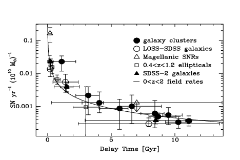
Figure 11.9: The type Ia supernovae delay time distribution (Maoz & Mannucci 2012).

It is clear from this figure that a significant fraction of type Ia supernovae explode at very large times (\(\gtrsim 5\,\mathrm{Gyr}\)) after star formation. However, while the data at delay times below 1 Gyr are sparse, it is also clear that the rate of explosions is highest at the shortest delay times. The solid curve shows a \(t^{-1}\) decay of the supernova rate, which fits the data well.

Theoretically, we expect a broad distribution of delay times in both the single- and double-degenerate scenarios. In the single-degenerate scenario, the delay time distribution is mostly determined by the requirement that the accretion rate onto the white dwarf has to be just so (\(\dot{M} \approx 10^{-7}\,M_\odot\,\mathrm{yr}^{-1}\); Nomoto 1982) for the white dwarf to stably grow in mass. This leads the delay times to range from a few hundred Myr to a few Gyr, with an exponential decrease at shorter and longer delay times (Greggio 2005; Bours et al. 2013).

In the double-degenerate scenario, a double-white-dwarf binary has to form through a complex process of binary evolution that culminates in a common-envelope phase and the loss of the envelope. The long delay time behavior (\(\gtrsim 1\,\mathrm{Gyr}\)) is determined by the time it takes to merge the resulting distribution of white-dwarf binary separations. Generically, the merger time dependence on the initial separation of the binary in either the gravitational-inspiral or direct-collision channel for binary white-dwarf mergers is so steep that it results in a delay time distribution \(\propto t^{-1}\) (Maoz et al. 2014). At shorter delay times, this power-law behavior has to break down, because each white dwarf in the binary’s main sequence progenitor must have a mass \(\lesssim 8\,M_\odot\) and lifetime \(\gtrsim 40\,\mathrm{Myr}\) to avoid exploding as a type II supernova, which therefore sets the absolute minimum time delay. Main-sequence stars with masses down to \(2\) to \(3\,M_\odot\) likely create white dwarfs that can be part of a type Ia supernova progenitor system and we should therefore expect the delay time distribution to fall below the \(t^{-1}\) merger-time behavior up to delay times equal to the main-sequence lifetimes of these low-mass progenitors (\(\approx 1\,\mathrm{Gyr}\) for a \(2\,M_\odot\) star or \(\approx 350\,\mathrm{Myr}\) for a \(3\,M_\odot\) star; Reid et al. 2002). The birth rate of white dwarfs is essentially set by the initial mass function (\(\mathrm{d}N/\mathrm{d}m \propto m^{-2.35}\) at the relevant masses \(m \gtrsim 2\,M_\odot\)) and the main-sequence lifetime (\(t \propto m^{-2.5}\)); for the power-law forms given, this gives a birth rate \(\mathrm{d}N/\mathrm{d}t \propto t^{-0.46} \approx t^{-1/2}\) (Pritchet et al. 2008). Because this falls below the \(t^{-1}\) merger-time behavior, it limits the rate of type Ia supernovae, so the delay time distribution for the double-degenerate scenario roughly looks like: (a) zero up \(40\,\mathrm{Myr}\), (b) \(\propto t^{-1/2}\) from the white-dwarf birth rate up to a time \(t_c\approx 350\,\mathrm{Myr}\) to \(1\,\mathrm{Gyr}\) depending on the lowest-mass main-sequence progenitor that contributes to an explosion, and (c) \(\propto t^{-1}\) from the steep dependence of the merger time on initial separation in the double white-dwarf binary (Maoz et al. 2014).

To be able to solve the non-instantaneous-recycling models for chemical evolution below, we require a SN Ia DTD that is an exponential starting at some minimum time or a sum of such exponentials (Weinberg et al. 2017). Thus, we need to approximate the observed DTD with a sum of a hopefully small number of exponentials. First, we need a good representation of the observed DTD. To determine that, we can use the observed DTD from Maoz et al. (2012), a recent determination based on type Ia supernovae observed with the SDSS-II survey (Frieman et al. 2008) in a parent sample of galaxies for which spectroscopic star-formation histories are available (Tojeiro et al. 2009). For the observed DTD, the total number of supernova explosions after 14 Gyr (the age of the Universe) per unit of stellar mass formed is \(N_{\mathrm{SN}}/M = 1.3\times10^{-3}\,M_\odot^{-1}\), a number which is uncertain at the \(50\%\) level (Maoz & Mannucci 2012). Let’s compare the data to a model for the DTD \(\Psi(\Delta t) \propto t^{-1.1}\), which is close to the best-fitting single power-law, and a model inspired by the expected double-degenerate DTD from the considerations above. The latter model has \(\Psi(t) \propto t^{-1/2}\) between the minimum delay time and the lifetime of the least massive star that contributes to type Ia SNe (we’ll use 570 Myr, which is the approximate lifetime of a \(2.5\,M_\odot\) star) and \(\Psi(t) \propto t^{-1.4}\), a slightly steeper dependence than the naively expected \(t^{-1}\) long-term behavior which fits the data better. For all models, we’ll assume that the minimum delay time is 50 Myr (assuming it takes at least 10 Myr to go from a \(8\,M_\odot\) binary white dwarf pair to an explosion). First, we implement the different DTD models:

def dtd_singlepower(dt,p=1.1,NSN_M=1.3e-3,mindt=0.05,maxdt=14.):
    """A single power-law t^-p DTD with total
    between 0 and 14 Gyr = NSN_M SN Ia / Mstar"""
    norm= (mindt**-(p-1)-maxdt**-(p-1))/(p-1)
    out= NSN_M/norm*dt**-p
    out[dt<mindt]= 0.
    return out
def dtd_brokenpower(dt,p1=0.5,p2=1.4,breakdt=0.57,
                    NSN_M=1.3e-3,mindt=0.05,maxdt=14.):
    """Broken power-law DTD with dt^-p1 at dt<breakdt
    and dt^-p2 at dt>breakdt"""
    norm= (mindt**-(p1-1)-breakdt**-(p1-1))/breakdt**-p1/(p1-1)\
        +(breakdt**-(p2-1)-maxdt**-(p2-1))/breakdt**-p2/(p2-1)
    out= numpy.zeros(len(dt))
    out[dt<breakdt]= (dt[dt<breakdt]/breakdt)**-p1
    out[dt>=breakdt]= (dt[dt>=breakdt]/breakdt)**-p2
    out[dt<mindt]= 0.
    return out*NSN_M/norm
def dblexp_approx(dt,hdt1=0.4,hdt2=3.3,
                  NSN_M=1.3e-3,mindt=0.05,maxdt=14.):
    """A DTD that is a sum of two equally-weighted exponentials"""
    out=  numpy.exp(-dt/hdt1)/hdt1/(numpy.exp(-mindt/hdt1)-numpy.exp(-maxdt/hdt1))/2.
    out+= numpy.exp(-dt/hdt2)/hdt2/(numpy.exp(-mindt/hdt2)-numpy.exp(-maxdt/hdt2))/2.
    out[dt<mindt]= 0.
    return out*NSN_M

and then we plot them versus the data in the left panel of Figure 11.10.

from matplotlib.ticker import FuncFormatter
data_dt= numpy.array([0.21,1.41,8.2])
data_dtd= numpy.array([140,25.1,1.83])*1e-5
data_dtd_err= numpy.array([30,6.3,0.42])*1e-5
data_cumdtd_x= numpy.array([0.42,2.4,14.])
data_cumdtd_y= numpy.cumsum(data_dtd*data_cumdtd_x)
data_cumdtd_y_err= numpy.sqrt(numpy.cumsum(data_dtd_err**2.*data_cumdtd_x))
figure(figsize=(12,5))
subplot(1,2,1)
dts= numpy.linspace(0.051,14.,201)
loglog(dts,dtd_singlepower(dts),
      label=r'$\propto t^{-1.1}$')
loglog(dts,dtd_brokenpower(dts),
      label=r'$\propto \begin{cases} t^{-0.5}\,,& t < 0.57\,\mathrm{Gyr}\\ t^{-1.4}\,,& t \geq 0.57\,\mathrm{Gyr}\end{cases}$')
loglog(dts,dblexp_approx(dts),
      label=r'$\mathrm{exp.\ approx.}$')
errorbar(data_dt,data_dtd,yerr=data_dtd_err,marker='o',color='k',
        ls='none')
xlabel(r'$\Delta t\,(\mathrm{Gyr})$')
ylabel(r'$\Psi\,(\mathrm{SNe\ Ia}\ \mathrm{Gyr}^{-1}\,M_\odot^{-1})$')
gca().xaxis.set_major_formatter(FuncFormatter(
                lambda y,pos: (r'${{:.{:1d}f}}$'.format(int(\
                    numpy.maximum(-numpy.log10(y),0)))).format(y)))
legend(frameon=False,fontsize=18.,loc='lower left')
subplot(1,2,2)
data_cumdtd_x= numpy.array([0.42,2.4,14.])
# integration interval for each observation
intdt= numpy.hstack((data_cumdtd_x[0],numpy.diff(data_cumdtd_x)))
data_cumdtd_y= numpy.cumsum(data_dtd*intdt)
data_cumdtd_y_err= numpy.sqrt(numpy.cumsum(data_dtd_err**2.*intdt**2.))
dts= numpy.linspace(0.0,14.,1001)
d_dt= dts[1]-dts[0]
plot(dts,numpy.cumsum(dtd_singlepower(dts))*d_dt,
    label=r'$\propto t^{-1.1}$')
plot(dts,numpy.cumsum(dtd_brokenpower(dts))*d_dt,
    label=r'$\propto \begin{cases} t^{-0.5}\,,& t < 0.57\,\mathrm{Gyr}\\ t^{-1.4}\,,& t \geq 0.57\,\mathrm{Gyr}\end{cases}$')
plot(dts,numpy.cumsum(dblexp_approx(dts))*d_dt,
    label=r'$\mathrm{exp.\ approx.}$')
errorbar(data_cumdtd_x,data_cumdtd_y,yerr=data_cumdtd_y_err,marker='o',color='k',
        ls='none')
axhline(1.3e-3/2.,color='0.7',ls='--')
ylim(-0.000095,0.001495)
xlabel(r'$\Delta t\,(\mathrm{Gyr})$')
ylabel(r'$\int\,\mathrm{d}\Delta t\Psi\,(\mathrm{SNe\ Ia}\ M_\odot^{-1})$')
legend(frameon=False,fontsize=18.,loc='lower right')
tight_layout();

Figure 11.10: Models for the type Ia supernovae delay time distribution compared to data from Maoz et al. (2012).

We see that the broken power-law model fits better, because the data indicate a steeper drop at \(t > 1\,\mathrm{Gyr}\) than would be expected from a single power law. For the effect of type Ia supernova enrichment on galactic chemical evolution, the cumulative number of explosions is important, so we compare the different models to the data as cumulative functions as well in the right panel of Figure 11.10. This again shows that there are more late-time explosions in the single power-law model than in the physically-motivated model. The single-power model is in slight tension with the data at \(\Delta t \approx 2\,\mathrm{Gyr}\). The dashed line indicates half of the supernova explosions that will happen; all models agree that these happen within 1 Gyr.

Because the broken power-law model compares better to the data, we will use that in the following sections. The figures above also show the best approximation of the broken power-law DTD as a sum of equally-weighted exponentials (there is no need for the exponentials to have the same contribution to the total number of supernova explosions, but it is simply convenient for the expressions below). This approximation has exponentials with decay time scales \(\tau = 0.4\,\mathrm{Gyr}\) and \(3.3\,\mathrm{Gyr}\).

Armed with the SN Ia DTD, we can model how SN Ia yields are distributed in time. For example, a single type Ia supernova produces \(m_{\mathrm{Fe}}^{\mathrm{Ia}} \approx 0.77\,M_\odot\) of iron (Iwamoto et al. 1999). To get the differential or cumulative yield of iron from type Ia supernovae, we can therefore simply multiply the curves above by \(m_{\mathrm{Fe}}^{\mathrm{Ia}}\). The total yield of iron 14 Gyr after star formation just from SNe Ia is then \(p_{\mathrm{Fe}}^{\mathrm{Ia}} \approx 0.001\). This is about the same as the total iron yield from core-collapse supernovae, which is \(p_{\mathrm{Fe}}^{\mathrm{II}} \approx 0.0011\) (Chieffi & Limongi 2004). The long term yield of iron from different supernova channels is therefore the same, but all of the iron enrichment by core-collapse supernovae happens within 40 Myr, while the type Ia supernova enrichment occurs at 40 Myr and beyond, with about half of this part coming at \(\Delta t \gtrsim 1\,\mathrm{Gyr}\).

11.3.2. The delayed closed box model

To get started with understanding the impact of the delay in enrichment resulting from type Ia supernova explosions, we can re-visit the closed box model from Section 11.2.1 when taking enrichment delays into account. We will focus on understanding the evolution of the iron abundance in the ISM and the ratio of the abundance of a pure core-collapse element, such as oxygen or magnesium, to the iron abundance. For the core-collapse contribution, we will continue to use the instantaneous recycling approximation, that is, enrichment from core-collapse supernovae is assumed to happen immediately after star formation.

The evolution of the pure core-collapse element remains that of the classical closed box model, expressed in terms of the gas mass in Equation (11.6). To obtain the equation that describes the evolution of the iron mass in the ISM, we need to edit Equation (11.4). Iron enrichment occurs both through core-collapse supernovae, with a yield \(p_{\mathrm{Fe}}^\mathrm{II}\), and through type Ia supernovae explosions, with a yield that depends on the past star formation rate \(\dot{M}_*\). We will split the contributions of iron to the ISM into that coming from core-collapse supernovae and that from type Ia supernovae and we will track them separately. Therefore, we will consider the evolution of \(M_{\mathrm{Fe}}^{\mathrm{II}}\) and \(M_{\mathrm{Fe}}^{\mathrm{Ia}}\), the iron mass contributed by core-collapse supernovae and by type Ia, respectively. And similar we will consider the abundances \(Z_{\mathrm{Fe}}^{\mathrm{II}}\) and \(Z_{\mathrm{Fe}}^{\mathrm{Ia}}\). While in reality we can of course not know which type of supernova produced a given iron atom, for the purpose of the calculation it is useful to imagine that we can (e.g., pretend that different types of supernovae give rise to different isotopes of iron) and that we add them together in the end to obtain the total iron abundance. The evolution of \(Z_{\mathrm{Fe}}^{\mathrm{II}}\) is the same as that of the pure core-collapse element considered in the classical closed box model, using the yield \(p_{\mathrm{Fe}}^\mathrm{II}\).

To solve for the evolution of \(Z_{\mathrm{Fe}}^{\mathrm{Ia}}\), we need to include iron enrichment from all past episodes of star formation at a given time and add it to the evolution equation (11.4). At a time \(\Delta t\) after an instantaneous burst of star formation, \(m_{\mathrm{Fe}}^{\mathrm{Ia}}\,\Psi(\Delta t)\) per unit time of iron is added to the ISM from type Ia supernovae explosions (where \(m_{\mathrm{Fe}}^{\mathrm{Ia}}\) is the mass of iron produced by a single SN Ia and \(\Psi(\Delta t)\) is the delay time distribution). To obtain the total yield of iron from past star formation at time \(t\), we therefore add up the yields from all past star formation. Using the notation from Section 11.2.1, we write this as \begin{equation}\label{eq-chemev-delayclosed-firstdMZFe} \dot{M}_{Z_{\mathrm{Fe}}^{\mathrm{Ia}},*+} = m_{\mathrm{Fe}}^{\mathrm{Ia}}\,\int_0^t \mathrm{d} t'\,\dot{M}_*(t')\,\Psi(t-t')\,. \end{equation} We can write this in terms of the total yield \(p_{\mathrm{Fe}}^{\mathrm{Ia}}\) from type Ia supernovae. We defined this above as \(p_{\mathrm{Fe}}^{\mathrm{Ia}} = m_{\mathrm{Fe}}^{\mathrm{Ia}}\,\int_0^{14\,\mathrm{Gyr}}\mathrm{d}\Delta t\,\Psi(\Delta t)\), but because we will use exponential DTDs that fall off steeply beyond 14 Gyr, we can approximate this by extending the integral to infinity, in which case Equation (11.35) can be written as \begin{equation}\label{eq-chemev-delayclosed-seconddMZFe} \dot{M}_{Z_{\mathrm{Fe}}^{\mathrm{Ia}},*+} = p_{\mathrm{Fe}}^{\mathrm{Ia}}\,\langle \dot{M}_*\rangle(t)\,, \end{equation} where the DTD-averaged star formation rate \(\langle \dot{M}_*\rangle(t)\) is defined as \begin{equation}\label{eq-chemev-DTDavgSFH} \langle \dot{M}_*\rangle(t) ={\int_0^t \mathrm{d} t'\,\dot{M}_*(t')\,\Psi(t-t') \over \int_0^\infty \mathrm{d} t'\,\Psi(t')}\,. \end{equation} This DTD-averaged star-formation history replaces the instantaneous star-formation history in Equation (11.4). If the DTD were a delta function at \(t=0\), that is, for instantaneous recycling, \(\langle \dot{M}_*\rangle(t) = \dot{M}_*(t)\). If the DTD were a shifted delta function at some delay \(T\), then we would find \(\langle \dot{M}_*\rangle(t) = \dot{M}_*(t-T)\). That is, the iron enrichment at time \(t\) would be the yield times the amount of mass turned into stars at a time \(T\) in the past rather than today. For realistic type Ia DTDs, the DTD-averaged star-formation history gives the effective mass of stars formed in the past for the purpose of considering iron enrichment of the ISM, such that the iron enrichment can be written in the simple form of Equation (11.36).

The full evolution equation for \(M_{Z_{\mathrm{Fe}}^{\mathrm{Ia}}}\) is obtained by adding the decrease in \(M_{Z_{\mathrm{Fe}}^{\mathrm{Ia}}}\) from the metals incorporated into stars, which similar to before is simply \(\dot{M}_{Z_{\mathrm{Fe}}^{\mathrm{Ia}},*-} = -Z_{\mathrm{Fe}}^{\mathrm{Ia}}\,\dot{M}_*\) and therefore \begin{equation}\label{eq-chemev-delayclosed-dmZfull-1} \dot{M}_{Z_{\mathrm{Fe}}^{\mathrm{Ia}}} = p_{\mathrm{Fe}}^{\mathrm{Ia}}\,\langle \dot{M}_*\rangle(t) -Z_{\mathrm{Fe}}^{\mathrm{Ia}}\,\dot{M}_*\,. \end{equation} To make progress in solving this equation, we need to know the star-formation history \(\dot{M}_*\) so we can compute the DTD-averaged star formation rate. As we discussed in Section 11.2.1, the star formation rate is not uniquely determined unless we specify how efficiently gas turns into stars. To be able to solve for the evolution of \(Z_{\mathrm{Fe}}^{\mathrm{Ia}}\) analytically, the model from Section 11.2.1 with a constant star formation efficiency time scale \(\tau_*\) is convenient. We showed previously that this model, which has constant \(\tau_*\) defined in Equation (11.10), has a star-formation history given by Equation (11.11). We further assume that the DTD is exponential \begin{equation} \Psi(\Delta t)\propto \exp\left(-\left[\Delta t-\Delta t^{\mathrm{Ia}}_{\mathrm{min}}\right]/\tau_{\mathrm{Ia}}\right)\,,\quad \Delta t > \Delta t^{\mathrm{Ia}}_{\mathrm{min}}\,, \end{equation} where \(\Delta t^{\mathrm{Ia}}_{\mathrm{min}}= 50\,\mathrm{Myr}\) is the minimum delay time. The DTD-averaged star-formation history is then \begin{align} \langle \dot{M}_*\rangle(t) & ={M_g(0)\over\tau_*\,\tau_{\mathrm{Ia}}}\,e^{-{t-\Delta t^{\mathrm{Ia}}_{\mathrm{min}}\over \tau_{\mathrm{Ia}}}}\,\int_0^{t-\Delta t^{\mathrm{Ia}}_{\mathrm{min}}} \mathrm{d} t'\,e^{t'/\tilde{\tau}}=\dot{M}_*(t)\,{\tilde{\tau}\over\tau_{\mathrm{Ia}}}\,e^{\Delta t^{\mathrm{Ia}}_{\mathrm{min}}/\tau_*}\,\left[1-\exp\left(-{t-\Delta t^{\mathrm{Ia}}_{\mathrm{min}}\over\tilde{\tau}}\right)\right]\,,\label{eq-chemev-DTDMstar-closedbox} \end{align} where we have introduced \(\tilde{\tau}\) defined through \(\tilde{\tau}^{-1} = \tau_{\mathrm{Ia}}^{-1}-\tau_*^{-1}\) and the resulting expression holds for \(t > \Delta t^{\mathrm{Ia}}_{\mathrm{min}}\) (with \(\langle \dot{M}_*\rangle(t)=0\) at earlier times). Plugging this into Equation (11.38), we find that \begin{equation}\label{eq-chemev-delayclosed-dmZfull-2} \dot{M}_{Z_{\mathrm{Fe}}^{\mathrm{Ia}}} = \left\{p_{\mathrm{Fe}}^{\mathrm{Ia}}\,{\tilde{\tau}\over\tau_{\mathrm{Ia}}}\,e^{\Delta t^{\mathrm{Ia}}_{\mathrm{min}}/\tau_*}\,\left[1-\exp\left(-{t-\Delta t^{\mathrm{Ia}}_{\mathrm{min}}\over\tilde{\tau}}\right)\right] -Z_{\mathrm{Fe}}^{\mathrm{Ia}}\right\}\,\dot{M}_*\,. \end{equation} Following the same steps as in going from Equation (11.4) to Equation (11.5), we then have the evolution equation for \(\dot{Z}_{\mathrm{Fe}}^{\mathrm{Ia}}\) \begin{equation}\label{eq-chemev-delayclosed-dZdt} \dot{Z}_{\mathrm{Fe}}^{\mathrm{Ia}} = -p_{\mathrm{Fe}}^{\mathrm{Ia}}\,{\tilde{\tau}\over\tau_{\mathrm{Ia}}}\,e^{\Delta t^{\mathrm{Ia}}_{\mathrm{min}}/\tau_*}\,\left[1-\exp\left(-{t-\Delta t^{\mathrm{Ia}}_{\mathrm{min}}\over\tilde{\tau}}\right)\right] \,{\dot{M}_g\over M_g}\,. \end{equation} We can solve this equation simply through integrating both sides from \(t'=0\) to \(t'=t\), using that \(\dot{M}_g/ M_g = -1/\tau_*\) and that \(Z_{\mathrm{Fe}}^{\mathrm{Ia}} = 0\) up to \(t=\Delta t^{\mathrm{Ia}}_{\mathrm{min}}\): \begin{equation}\label{eq-chemev-delayclosed-Zt} Z_{\mathrm{Fe}}^{\mathrm{Ia}} = p_{\mathrm{Fe}}^{\mathrm{Ia}}\,{\tilde{\tau}\over\tau_{\mathrm{Ia}}\,\tau_*}\,e^{\Delta t^{\mathrm{Ia}}_{\mathrm{min}}/\tau_*}\,\left\{t-\Delta t^{\mathrm{Ia}}_{\mathrm{min}}-\tilde{\tau}\,\left[1-\exp\left(-{t-\Delta t^{\mathrm{Ia}}_{\mathrm{min}}\over\tilde{\tau}}\right)\right]\right\}\,, \end{equation} at \(t > \Delta t^{\mathrm{Ia}}_{\mathrm{min}}\) and zero at earlier times. That \(Z_{\mathrm{Fe}}^{\mathrm{Ia}}\) is zero until \(\Delta t^{\mathrm{Ia}}_{\mathrm{min}}\) makes sense, because it takes that long for the first SNe Ia to explode. Taylor expanding the exponential for \(t-\Delta t^{\mathrm{Ia}}_{\mathrm{min}} \ll \tilde{\tau}\) shows that \(Z_{\mathrm{Fe}}^{\mathrm{Ia}} \propto (t-\Delta t^{\mathrm{Ia}}_{\mathrm{min}})^2\) at small \(t-\Delta t^{\mathrm{Ia}}_{\mathrm{min}}\), so type Ia supernova enrichment turns on slowly.

To apply this model to the solar neighborhood abundance distribution, we need to set the parameters \(\tau_*\) and \(\tau_{\mathrm{Ia}}\). For simplicity, we will for now represent the DTD using a single exponential with \(\tau_{\mathrm{Ia}} = 1.5\,\mathrm{Gyr}\). As discussed below Equation (11.12), in the context of the closed box model we require that \(\tau_* \approx 4.5\,\mathrm{Gyr}\). We can then compare the evolution of \(Z_{\mathrm{Fe}}^{\mathrm{Ia}}\) to that of \(Z_{\mathrm{Fe}}^{\mathrm{II}}\), which is given by Equation (11.12) with \(p = p_{\mathrm{Fe}}^{\mathrm{II}} \approx 0.0011\). This is shown in Figure 11.11.

def Z_Fe_Ia_closedbox(t,p_Fe_Ia=0.001,tau_Ia=1.5,tau_star=4.5,mindt=0.05):
    tau_tilde= 1./(1./tau_Ia-1./tau_star)
    out= p_Fe_Ia*tau_tilde/tau_Ia/tau_star\
        *numpy.exp(mindt/tau_star)\
        *(t-mindt-tau_tilde*(1.-numpy.exp(-(t-mindt)/tau_tilde)))
    out[t<mindt]= 0.
    return out
def Z_Fe_II_closedbox(t,p_Fe_II=0.0011,tau_star=4.5):
    return p_Fe_II*t/tau_star
ts= numpy.linspace(0.,10.,201)
figure(figsize=(7,5))
plot(ts,Z_Fe_Ia_closedbox(ts),label=r'$\mathrm{Ia\ SNe}$')
plot(ts,Z_Fe_II_closedbox(ts),label=r'$\mathrm{II\ SNe}$')
xlabel(r'$t\,(\mathrm{Gyr})$')
ylabel(r'$Z_{\mathrm{Fe}}$')
legend(frameon=False,fontsize=18.);

Figure 11.11: Iron enrichment due to type Ia and type II supernovae in the closed-box model.

In the closed box model, the contribution from instantaneous core-collapse supernovae to the enrichment grows linearly in time, while that from the delayed type Ia supernovae turns on slowly. However, once it turns on, the type Ia enrichment increases faster with time and eventually overtakes the core-collapse contribution. Why and how this happens can be understood by looking at the behavior of Equation (11.42) at \(t \gg \tilde{\tau}\), using the fact that for \(\tau_* \gg \tau_{\mathrm{Ia}}\), \(\tilde{\tau} \approx \tau_{\mathrm{Ia}}\): \begin{equation} \dot{Z}_{\mathrm{Fe}}^{\mathrm{Ia}} \approx -p_{\mathrm{Fe}}^{\mathrm{Ia}}\,e^{\Delta t^{\mathrm{Ia}}_{\mathrm{min}}/\tau_*} \,{\dot{M}_g\over M_g}\,. \end{equation} Comparing this to Equation (11.5) which gives the behavior of \(\dot{Z}_{\mathrm{Fe}}^{\mathrm{II}}\), we see that the \(t \gg \tilde{\tau}\) behavior is essentially that of the instantaneous recycling approximation, but with the yield given by \(p_{\mathrm{Fe}}^{\mathrm{Ia}}\,e^{\Delta t^{\mathrm{Ia}}_{\mathrm{min}}/\tau_*}\) (to get quantitative agreement with the slope in the figure above, one needs to account for the \(\tilde{\tau} / \tau_{\mathrm{Ia}}\) factor as well). Physically, this happens because for \(\tau_* \gg \tau_{\mathrm{Ia}}\), all type Ia supernovae explode before the star-formation rate changes significantly and the DTD-averaged star-formation rate is therefore about the same as the instantaneous star-formation rate; thus, this situation is equivalent to an instantaneous recycling model.

In the opposite limit, where \(\tau_* \ll \tau_{\mathrm{Ia}}\) and star formation thus proceeds more rapidly than enrichment from type Ia supernovae, Equation (11.42) at \(t \gg \tilde{\tau}\) becomes \begin{equation} \dot{Z}_{\mathrm{Fe}}^{\mathrm{Ia}} \approx -p_{\mathrm{Fe}}^{\mathrm{Ia}}\,{\tau_*\over \tau_{\mathrm{Ia}}}\,e^{t/\tau_*} \,{\dot{M}_g\over M_g}\,, \end{equation} because now \(\tilde{\tau} \approx -\tau_*\). Thus, the effective yield (the part of the expression that multiplies \(\dot{M}_g/M_g\)) increases exponentially with time, leading to exponential growth of the iron abundance \(Z_{\mathrm{Fe}}^{\mathrm{Ia}} \approx (p_{\mathrm{Fe}}^{\mathrm{Ia}}\,\tau_*/\tau_{\mathrm{Ia}})\,e^{t/\tau_*}\). This leads to a very high iron abundance; for example, let’s compare the behavior of \(Z^{\mathrm{Ia}}_{\mathrm{Fe}}\) for \(\tau_*/\tau_{\mathrm{Ia}} = 3\) to that of \(\tau_*/\tau_{\mathrm{Ia}} = 1/3\) in Figure 11.12.

ts= numpy.linspace(0.,10.,201)
figure(figsize=(7,5))
semilogy(ts,Z_Fe_Ia_closedbox(ts,tau_star=4.5,tau_Ia=1.5),label=r'$\tau_*/\tau_{\mathrm{Ia}} = 3$')
semilogy(ts,Z_Fe_Ia_closedbox(ts,tau_star=0.5,tau_Ia=1.5),label=r'$\tau_*/\tau_{\mathrm{Ia}} = 1/3$')
xlabel(r'$t\,(\mathrm{Gyr})$')
ylabel(r'$Z^{\mathrm{Ia}}_{\mathrm{Fe}}$')
legend(frameon=False,fontsize=18.);

Figure 11.12: Iron enrichment due to type Ia supernovae for different star formation efficiency and delay-time time scales in the closed-box model.

We have had to switch to logarithmically-scaled axes here because the increase in the iron abundance is so fast for \(\tau_*/\tau_{\mathrm{Ia}} = 1/3\). Of course, this is not a physical model, because the mass in iron of the ISM cannot exceed the total mass of the ISM and therefore \(Z\leq 1\); the high \(Z\) obtained in this model breaks our assumption that \(Z \ll 1\). The physical reason for the exponential increase in the iron abundance when \(\tau_* \ll \tau_{\mathrm{Ia}}\) is that in this case the star formation rate has significantly dropped by the time many of the type Ia supernova explosions happen from earlier star formation. Thus, the DTD-averaged star-formation rate is much higher than the instantaneous star-formation rate, which leads to much higher effective yield than would be expected if enrichment were instantaneous. In the closed box model this effect is amplified by the fact that the gas mass has also decreased significantly between when the stars formed and when they explode as supernovae; the same amount of iron produced by these supernovae then leads to much higher fractional increase of the ISM’s iron abundance.

To confront the predictions from the closed box model with enrichment from both instantaneous core-collapse supernovae and delayed type Ia supernovae, we can calculate the expected relation between the iron abundance \(Z_{\mathrm{Fe}}\) and the relative abundance of oxygen to that of iron \(Z_{\mathrm{O}}/Z_{\mathrm{Fe}}\). For this, we need to compute \(Z_{\mathrm{O}}\), which assuming that oxygen is only produced by type II supernovae follows Equation (11.12) with \(p = p_{\mathrm{O}}^{\mathrm{II}} \approx 0.016\) (Chieffi & Limongi 2004). To obtain the iron abundance \(Z_{\mathrm{Fe}}\), we add up contributions from the type Ia and type II enrichment channels: \(Z_{\mathrm{Fe}} = Z_{\mathrm{Fe}}^{\mathrm{II}}+Z_{\mathrm{Fe}}^{\mathrm{Ia}}\). We will also consider the two-exponential approximation to the more realistic type Ia DTD from Section 11.3.1, which splits the DTD into two equal parts with decay time scales \(\tau_{\mathrm{Ia},1}\) and \(\tau_{\mathrm{Ia},2}\). In this case, \(Z_{\mathrm{Fe}} = Z_{\mathrm{Fe}}^{\mathrm{II}}+Z_{\mathrm{Fe}}^{\mathrm{Ia},1}+Z_{\mathrm{Fe}}^{\mathrm{Ia},2}\), where \(Z_{\mathrm{Fe}}^{\mathrm{Ia},i}\) is the contribution from type Ia supernovae computed using the \(\tau_{\mathrm{Ia},i}\) exponential. Observationally, abundances and abundance ratios are expressed as logarithmic quantities normalized to the solar abundance, with the additional complication that abundances are weighted by number of atoms rather than by mass. That is, the observed iron abundance \([\mathrm{Fe/H}]\) is defined as \begin{equation} [\mathrm{Fe/H}] = \log_{10}\left(N_{\mathrm{Fe}}/N_{\mathrm{H}}\over N_{\mathrm{Fe},\odot}/N_{\mathrm{H},\odot}\right)\,, \end{equation} and the oxygen-to-iron ratio \([\mathrm{O/Fe}]\) is \begin{equation} [\mathrm{O/Fe}] = \log_{10}\left(N_{\mathrm{O}}/N_{\mathrm{Fe}}\over N_{\mathrm{O},\odot}/N_{\mathrm{Fe},\odot}\right) = [\mathrm{O/H}]-[\mathrm{Fe/H}]\,. \end{equation}

Because the quantity \(Z_{\mathrm{Fe}}\) that we compute is the mass of iron relative to the total mass rather than the number of iron atoms, the easiest way to convert \(Z_{\mathrm{Fe}}\) to \([\mathrm{Fe/H}]\) is to express the solar iron abundance as a relative mass of iron in the Sun as well (and similar for \(Z_{\mathrm{O}}\)). The abundances of different elements in the Sun is typically given on a logarithmic scale where the number of hydrogen atoms is set to \(10^{12}\) (see Section 11.1 above), the abundance by number of element \(X\) is \(x = 12 + \log_{10}\left(\mathrm{X/H}\right)\) and the conversion to a logarithmic mass fraction is \begin{equation}\label{eq-chemev-abundance-weight-from-abundance-number} \log_{10} Z_{\mathrm{X},\odot} = x_i-12 + \log_{10} \mu + \log_{10} 0.71\,, \end{equation} where \(\mu\) is the atomic weight of element \(X\) and \(0.71\) is the mass fraction of hydrogen in the Sun. The atomic weight of iron is 55.85 and the abundance of iron in the Sun is \(x_{\mathrm{Fe}} = 7.5\) while the atomic weight of oxygen is 16 and its abundance in the Sun is \(x_{\mathrm{O}} = 8.69\) (Asplund et al. 2009), so we have that \begin{align}\label{eq-chemev-solarO} \log_{10} Z_{\mathrm{Fe},\odot} & = -2.90\,;\quad \log_{10} Z_{\mathrm{O},\odot} = -2.25\,. \end{align} With these numbers we can then compute \([\mathrm{Fe/H}] = \log_{10} Z_{\mathrm{Fe}} - \log_{10} Z_{\mathrm{Fe},\odot}\) and similar for oxygen. We can then compute the relation between \([\mathrm{O/Fe}]\) and \([\mathrm{Fe/H}]\) (the track) for our two different DTD representations in the delayed closed box model and display this in Figure 11.13 below. We see that at low \([\mathrm{Fe/H}]\), the relative abundance of oxygen to that of iron is constant and forms a plateau. This occurs, because at early times (low \([\mathrm{Fe/H}]\)), enrichment by type Ia supernovae is negligible and both iron and oxygen are enriched through instantaneous type II supernova enrichment. The relative abundance is then simply equal to the relative ratio of the core-collapse yields for oxygen and iron. However, after about 1 Gyr, enrichment from type Ia supernovae becomes an important contributor to \(Z_{\mathrm{Fe}}\) and the iron abundance therefore starts to increase faster, driving down the relative ratio of oxygen to iron. The exact way in which this happens depends on the DTD, as the figure above shows, although the exact representation of the DTD only makes a small quantitative difference in the location in the track, with the qualitative behavior independent on the details of the DTD. From now on, we will only consider the two exponential approximation to the broken-power-law DTD model.

We can compare the predicted track to data on the abundance ratios of stars in the solar neighborhood. The oxygen abundance is tricky to measure using stellar spectra, because oxygen absorption lines are rare and difficult to interpret in the optical region of the electromagnetic spectrum where most high-resolution spectrographs operate. But we will use a sample of \(\approx 800\) solar-neighborhood stars from Ramirez et al. (2013), which we can load from the Vizier service using the function to download catalogs from Vizier in Section 12.2.2, repeated here:

# vizier.py: download catalogs from Vizier
import sys
from pathlib import Path
import shutil
import tempfile
from ftplib import FTP
import subprocess
_ERASESTR= "                                                                                "
def vizier(cat,filePath,ReadMePath,
           catalogname='catalog.dat',readmename='ReadMe'):
    """
    NAME:
       vizier
    PURPOSE:
       download a catalog and its associated ReadMe from Vizier
    INPUT:
       cat - name of the catalog (e.g., 'III/272' for RAVE, or J/A+A/... for journal-specific catalogs)
       filePath - path of the file where you want to store the catalog (note: you need to keep the name of the file the same as the catalogname to be able to read the file with astropy.io.ascii)
       ReadMePath - path of the file where you want to store the ReadMe file
       catalogname= (catalog.dat) name of the catalog on the Vizier server
       readmename= (ReadMe) name of the ReadMe file on the Vizier server
    OUTPUT:
       (nothing, just downloads)
    HISTORY:
       2016-09-12 - Written as part of gaia_tools - Bovy (UofT)
       2017-09-12 - Copied to galdyncourse (yes, same day!) - Bovy (UofT)
       2019-12-20 - Copied directly into notes to avoid additional dependency - Bovy (UofT)
    """
    _download_file_vizier(cat,filePath,catalogname=catalogname)
    _download_file_vizier(cat,ReadMePath,catalogname=readmename)
    catfilename= Path(catalogname).name
    with open(ReadMePath,'r') as readmefile:
        fullreadme= ''.join(readmefile.readlines())
        if catfilename.endswith('.gz') and not catfilename in fullreadme:
            # Need to gunzip the catalog
            try:
                subprocess.check_call(['gunzip',filePath])
            except subprocess.CalledProcessError as e:
                print("Could not unzip catalog %s" % filePath)
                raise
    return None

def _download_file_vizier(cat,filePath,catalogname='catalog.dat'):
    sys.stdout.write('\r'+"Downloading file %s from Vizier ...\r" \
                         % (Path(filePath).name))
    sys.stdout.flush()
    try:
        # make all intermediate directories
        os.makedirs(Path(filePath).parent)
    except OSError: pass
    # Safe way of downloading
    downloading= True
    interrupted= False
    file, tmp_savefilename= tempfile.mkstemp()
    os.close(file) #Easier this way
    ntries= 1
    while downloading:
        try:
            ftp= FTP('cdsarc.u-strasbg.fr')
            ftp.login()
            ftp.cwd(str(Path('pub') / 'cats' / cat))
            with open(tmp_savefilename,'wb') as savefile:
                ftp.retrbinary('RETR %s' % catalogname,savefile.write)
            shutil.move(tmp_savefilename,filePath)
            downloading= False
            if interrupted:
                raise KeyboardInterrupt
        except:
            raise
            if not downloading: #Assume KeyboardInterrupt
                raise
            elif ntries > _MAX_NTRIES:
                raise IOError('File %s does not appear to exist on the server ...' % (Path(filePath).name))
        finally:
            if Path(tmp_savefilename).exists():
                os.remove(tmp_savefilename)
        ntries+= 1
    sys.stdout.write('\r'+_ERASESTR+'\r')
    sys.stdout.flush()
    return None

We first write a function to download and process the catalog:

import os
from pathlib import Path
from astropy.io import ascii
from astropy.table import join as table_join
_CACHE_BASEDIR= Path(os.getenv('HOME')) / '.galaxiesbook' / 'cache'
_CACHE_VIZIER_DIR= _CACHE_BASEDIR / 'vizier'
_RAMIREZ_VIZIER_NAME= 'J/ApJ/764/78'
def read_sn_o_abu(verbose=False):
    """
    NAME:
       read_sn_o_abu
    PURPOSE:
       read the Ramirez et al. catalog of oxygen abundances of
       stars in the solar neighborhood
    INPUT:
       verbose= (False) if True, be verbose
    OUTPUT:
       pandas dataframe
    HISTORY:
       2020-11-20 - Written - Bovy (UofT)
    """
    # Generate file path and name
    tPath= _CACHE_VIZIER_DIR / 'cats'
    for directory in _RAMIREZ_VIZIER_NAME.split('/'):
        tPath = tPath / directory
    # First download table with [Fe/H]
    filePath_FEH= tPath / 'table4.dat'
    readmePath= tPath / 'ReadMe'
    # download the file
    if not filePath_FEH.exists():
        vizier(_RAMIREZ_VIZIER_NAME,filePath_FEH,readmePath,
               catalogname='table4.dat',readmename='ReadMe')
    # Then table with [O/H]
    filePath_OH= tPath / 'table6.dat'
    # download the file
    if not filePath_OH.exists():
        vizier(_RAMIREZ_VIZIER_NAME,filePath_OH,readmePath,
               catalogname='table6.dat',readmename='ReadMe')
    # Read with astropy
    table_feh= ascii.read(str(filePath_FEH),readme=str(readmePath),format='cds')
    table_oh= ascii.read(str(filePath_OH),readme=str(readmePath),format='cds')
    out= table_join(table_feh,table_oh)
    out= out[out['Sample'] == 'main']
    return out.to_pandas()

and then a function to plot the \([\mathrm{O/Fe}]\) versus \([\mathrm{Fe/H}]\) distribution of the stars:

def plot_sn_ofe_feh(xrange=[-2.05,0.65],yrange=[-0.15,0.6]):
    sndata= read_sn_o_abu()
    sndata= sndata[(sndata['e_[Fe/H]2'] < 0.15)*(sndata['e_[O/H]N'] < 0.05)]
    data_plot = plot(sndata['[Fe/H]2'],sndata['[O/H]N']-sndata['[Fe/H]2'],
                     'ko',ms=2.,label=r'$\mathrm{data}$')
    xlabel(r'$[\mathrm{Fe/H}]$')
    ylabel(r'$[\mathrm{O/Fe}]$')
    xlim(*xrange)
    ylim(*yrange)
    return data_plot

We can then confront the delayed closed box model with \(\tau_* = 4.5\,\mathrm{Gyr}\) with these data in Figure 11.13.

def feh_closedbox(t,p_Fe_Ia=0.001,p_Fe_II=0.0011,
                  tau_Ia=0.4,tau_Ia_2=3.3,mindt=0.05,
                  tau_star=4.5,solar_Fe=7.5):
    tau_tilde= 1./(1./tau_Ia-1./tau_star)
    out= p_Fe_Ia*tau_tilde/tau_Ia/tau_star\
        *numpy.exp(mindt/tau_star)\
        *(t-mindt-tau_tilde*(1.-numpy.exp(-(t-mindt)/tau_tilde)))
    # Second exponential Ia component
    if not tau_Ia_2 is None:
        out/= 2.
        tau_tilde= 1./(1./tau_Ia_2-1./tau_star)
        out+= p_Fe_Ia/2.*tau_tilde/tau_Ia_2/tau_star\
            *numpy.exp(mindt/tau_star)\
            *(t-mindt-tau_tilde*(1.-numpy.exp(-(t-mindt)/tau_tilde)))
    out[t<mindt]= 0.
    # Add CCSN contribution
    out+= p_Fe_II*t/tau_star
    # Convert to [Fe/H]
    logZFe_solar= -2.90+solar_Fe-7.50
    return numpy.log10(out)-logZFe_solar
def oh_closedbox(t,p_O_II=0.016,
                 tau_star=4.5,solar_O=8.69):
    # Just CCSN contribution
    out= p_O_II*t/tau_star
    # Convert to [O/H]
    logZO_solar= -2.25+solar_O-8.69
    return numpy.log10(out)-logZO_solar
ts= numpy.geomspace(1e-3,10.,201)
figure(figsize=(7,5))
line_data = plot_sn_ofe_feh()
line_twoexp = plot(feh_closedbox(ts),oh_closedbox(ts)-feh_closedbox(ts),
     label=r'$\Psi(\Delta t) \propto \begin{cases} t^{-0.5}\,,& t < 0.57\,\mathrm{Gyr}\\ t^{-1.4}\,,& t \geq 0.57\,\mathrm{Gyr}\end{cases}$')
line_oneexp = plot(feh_closedbox(ts,tau_Ia=1.5,tau_Ia_2=None),
     oh_closedbox(ts)-feh_closedbox(ts,tau_Ia=1.5,tau_Ia_2=None),
     zorder=-1,
     label=r'$\Psi(\Delta t) \propto e^{-\Delta t / [1.5\,\mathrm{Gyr}]}$')
xlabel(r'$[\mathrm{Fe/H}]$')
ylabel(r'$[\mathrm{O/Fe}]$')
legend(handles=[line_data[0],line_oneexp[0],line_twoexp[0]],
       frameon=True,fontsize=15.25,loc='lower left',
       framealpha=0.,edgecolor='w');

Figure 11.13: Chemical evolution track in [O/Fe] vs. [Fe/H] in the closed-box model compared to solar-neighborhood data from Ramirez et al. (2013).

We see that while the plateau at low \([\mathrm{Fe/H}]\) is indeed at the upper limit of \([\mathrm{O/Fe}]\) in the data, the drop towards lower \([\mathrm{O/Fe}]\) at higher \([\mathrm{Fe/H}]\) starts at too low \([\mathrm{Fe/H}]\) and is too slow. While the data go down to \([\mathrm{O/Fe}] \approx 0\) and perhaps a bit below (which is expected, because the Sun has to form at some point and the Sun has \([\mathrm{O/Fe}] = 0\)), the delayed closed box model only reaches \([\mathrm{O/Fe}]\approx 0.2\). While the exact values of the plateau and the final \([\mathrm{O/Fe}]\) depend on the yields from the different types of supernovae, which are somewhat uncertain, the discrepancy is beyond that which can be easily explained through theoretical uncertainties and the shallow drop in particular is in strong conflict with the data. Thus, the closed box model can neither explain the observed metallicity distribution (the G dwarf problem, Section 11.2.2) or the track of solar-neighborhood stars in \([\mathrm{O/Fe}]\) versus \([\mathrm{Fe/H}]\)!

11.3.3. The delayed leaky box model

We can extend the closed box model with delayed type Ia supernova enrichment with outflows of gas and derive the delayed version of the leaky box model from Section 11.2.3. Again defining the outflow efficiency \(\eta \equiv \dot{M}_{\mathrm{outflow}}/\dot{M}_*\) and assuming it to be constant and combining this now with the constant star-formation-efficiency model (Equation 11.10; \(\tau_* = M_g/\dot{M}_*\), the evolution of the gas mass becomes \(\dot{M}_g = -(1+\eta) M_g/\tau_*\). The gas mass therefore evolves as \(M_g(t) = M_g(0)\exp\left(-t/\tau_{\mathrm{dep}}\right)\), where \(\tau_{\mathrm{dep}} = \tau_*/(1+\eta)\) is the depletion time scale. The star formation rate follows from \(\tau_* = M_g/\dot{M}_*\) \begin{equation} \dot{M}_*(t) = {M_g(0)\over \tau_*}\,e^{-t/\tau_{\mathrm{dep}}}\,. \end{equation} For this star formation rate, the DTD-averaged star formation rate is still given by the expression in Equation (11.40), except that now \(\tilde{\tau}^{-1} = \tau_{\mathrm{Ia}}^{-1}-\tau_{\mathrm{dep}}^{-1}\). The evolution equation for the Ia contribution to iron, \(\dot{M}_{Z_{\mathrm{Fe}}^{\mathrm{Ia}}}\) gains an outflow contribution as in Equation (11.23) and thus becomes \begin{equation}\label{eq-chemev-delayleaky-dmZfull-1} \dot{M}_{Z_{\mathrm{Fe}}^{\mathrm{Ia}}} = p_{\mathrm{Fe}}^{\mathrm{Ia}}\,\langle \dot{M}_*\rangle(t) -(1+\eta)\,Z_{\mathrm{Fe}}^{\mathrm{Ia}}\,\dot{M}_*\,. \end{equation} Similar to going from \(\dot{M}_Z\) in Equation (11.24) to \(\dot{Z}\) in Equation (11.25) for the classical leaky box model, the evolution equation for \(\dot{Z}_{\mathrm{Fe}}^{\mathrm{Ia}}\) is then the same expression as that in Equation (11.42) but replacing the yield \(p_{\mathrm{Fe}}^{\mathrm{Ia}}\) with the effective yield \(p_{\mathrm{Fe}}^{\phantom{\,}_{'},\mathrm{Ia}} = p_{\mathrm{Fe}}^{\mathrm{Ia}} / (1+\eta)\) and now \(\dot{M}_g/ M_g = -1/\tau_{\mathrm{dep}}\). The solution of this equation is then also given by the expression in Equation (11.43) with the same \(p_{\mathrm{Fe}}^{\mathrm{Ia}} \rightarrow p_{\mathrm{Fe}}^{\phantom{\,}_{'},\mathrm{Ia}}\) replacement and additionally replacing \(\tau_* \rightarrow \tau_{\mathrm{dep}} = \tau_*/(1+\eta)\). Thus, similar to the relation between the classical closed and leaky box models, the delayed leaky box model has a similar evolution as the delayed closed box model, but with effective yield and evolution time scale that are lower by \(1/[1+\eta]\) due to outflows. As discussed in Section 11.2.3, we can treat instantaneous recycling of material at the stars’ birth abundance through stellar winds in the same way, leading to an effective yield \(p_{\mathrm{Fe}}^{\phantom{\,}_{'},\mathrm{Ia}} = p_{\mathrm{Fe}}^{\mathrm{Ia}} / (1+\eta-r)\), where \(r\) is the recycling fraction, which is about 0.4. In this more general case, the depletion time scale is then \(\tau_{\mathrm{dep}} = \tau_*/(1+\eta-r)\).

The same relation between the leaky and closed box models holds for the evolution of the type II supernova contribution to Fe and to that of oxygen, and the evolution of those \(Z_{\mathrm{Fe}}^{\mathrm{II}}\) and \(Z_{\mathrm{O}}^{\mathrm{II}}\) is therefore given by Equation (11.12) with yield parameter \(p_{\mathrm{X}}^{\mathrm{II}} \rightarrow p_{\mathrm{X}}^{\phantom{\,}_{'},\mathrm{II}} = p_{\mathrm{X}}^{\mathrm{II}}/(1+\eta-r)\). To compare the leaky box model with recycling to the data on the relation between \([\mathrm{O/Fe}]\) and \([\mathrm{Fe/H}]\) in the solar neighborhood, we need to set \(\tau_*\) such that \(M_*/M_g \approx 10\) at \(t=10\,\mathrm{Gyr}\); it is left as an exercise to show that this requires \(\tau_{\mathrm{dep}} = t/\ln\left([1+\eta-r]\,M_*/M_g +1\right)\) and therefore \(\tau_* \approx 9\,\mathrm{Gyr}\). This is twice as large as the \(\tau_* = 4.5\,\mathrm{Gyr}\) that we required in the closed box model. That the required \(\tau_*\) to obtain a given ratio of stellar-to-gas mass is larger in the leaky box makes sense, because when some of the gas is lost to outflows, we need to make fewer stars out of the initial gas supply to get to the same ratio and the star formation efficiency can therefore be lower (and its time scale larger). We compare the leaky box model to the data from Ramirez et al. (2013) in Figure 11.14.

ts= numpy.linspace(0.,10.,201)
def feh_leakybox(t,p_Fe_Ia=0.001,p_Fe_II=0.0011,
                 tau_Ia=0.4,tau_Ia_2=3.3,mindt=0.05,
                 tau_star=4.5,solar_Fe=7.5,
                 eta=2.5,r=0.4):
    # Equivalent to closed box with p' = p/(1+eta-r)
    # and tau_star'= tau_star/(1.+eta-r)
    return feh_closedbox(t,p_Fe_Ia=p_Fe_Ia/(1.+eta-r),
                         p_Fe_II=p_Fe_II/(1.+eta-r),
                         tau_Ia=tau_Ia,tau_Ia_2=tau_Ia_2,
                         mindt=mindt,
                         tau_star=tau_star/(1.+eta-r),
                         solar_Fe=solar_Fe)
def oh_leakybox(t,p_O_II=0.016,
                tau_star=4.5,solar_O=8.69,
                eta=2.5,r=0.4):
    # Equivalent to closed box with p' = p/(1+eta-r)
    # and tau_star'= tau_star/(1.+eta-r)
    return oh_closedbox(t,p_O_II=p_O_II/(1.+eta-r),
                         tau_star=tau_star/(1.+eta-r),
                         solar_O=solar_O)
ts= numpy.geomspace(1e-3,10.,201)
figure(figsize=(7,5))
plot_sn_ofe_feh(xrange=[-2.19,0.65],yrange=[-0.34,0.6])
plot(feh_closedbox(ts),oh_closedbox(ts)-feh_closedbox(ts),
    lw=2.,label=r'$\mathrm{closed\ box}; \tau_* = 4.5\,\mathrm{Gyr}$')
plot(feh_leakybox(ts),oh_leakybox(ts)-feh_leakybox(ts),
     lw=2.,label=r'$\mathrm{leaky\ box}; \eta=2.5,\ r=0.4,\ \tau_* = 4.5\,\mathrm{Gyr}$')
plot(feh_leakybox(ts,tau_star=9.),
     oh_leakybox(ts,tau_star=9.)-feh_leakybox(ts,tau_star=9.),
     lw=2.,label=r'$\mathrm{leaky\ box}; \eta=2.5,\ r=0.4,\ \tau_* = 9.0\,\mathrm{Gyr}$')
xlabel(r'$[\mathrm{Fe/H}]$')
ylabel(r'$[\mathrm{O/Fe}]$')
legend(frameon=False,fontsize=18,loc='lower left');

Figure 11.14: Like Figure 11.13, but for leaky-box models.

As expected, the leaky box predictions are similar to those of the closed box model, except that they are shifted to lower metallicities because the effective yields are smaller than the true yields by the factor of \(1/(1+\eta-r)\). It is clear that adding outflows to the closed box model does not improve the agreement with the data on the abundance ratios.

11.3.4. The delayed accreting box

\label{sec-chemev-delayedaccretion}

Next, we can add inflows of gas to the model as well and consider the accreting box model from Section 11.2.4 with delayed type Ia supernova enrichment. As we saw in that section, adding inflows of gas is a good way to solve the G dwarf problem and if inflows can also lead to better agreement on the \([\mathrm{O/Fe}]\) versus \([\mathrm{Fe/H}]\) distribution in the solar neighborhood, the inflow model would become even more compelling.

As in Section 11.2.4, we will assume that the gas mass is constant in time: \(M_g(t) = M_g(0)\), such that inflows balance the loss of gas due to outflows and the consumption of gas by star formation that is not returned through recycling. Because the gas mass is constant, the star formation rate is constant as well for a constant star formation efficiency time scale \(\tau_*\) \begin{equation}\label{eq-chemev-dotmstar-delayedaccretingbox} \dot{M}_* = {M_g \over \tau_*}\,. \end{equation} For a constant star formation rate, the DTD-averaged star formation rate follows from its definition in Equation (11.37). For an exponentially declining DTD with decay time scale \(\tau_{\mathrm{Ia}}\) and minimum delay time \(\Delta t^{\mathrm{Ia}}_{\mathrm{min}}\) \begin{align} \langle \dot{M}_*\rangle(t) & ={M_g\over\tau_*}\,\left[1-\exp\left(-{t-\Delta t^{\mathrm{Ia}}_{\mathrm{min}}\over \tau_{\mathrm{Ia}}}\right)\right]\,.\label{eq-chemev-DTDMstar-accretingbox} \end{align} The evolution equation of \(\dot{M}_{Z_{\mathrm{Fe}}^{\mathrm{Ia}}}\) is still given by Equation (11.51) (we will immediately skip to the model that includes outflows and recycling) and plugging in the DTD-averaged star formation rate from Equation (11.53), we get \begin{equation}\label{eq-chemev-delayaccrete-dmZfull-1} \dot{M}_{Z_{\mathrm{Fe}}^{\mathrm{Ia}}} = \left\{p_{\mathrm{Fe}}^{\mathrm{Ia}}\,\left[1-\exp\left(-{t-\Delta t^{\mathrm{Ia}}_{\mathrm{min}}\over \tau_{\mathrm{Ia}}}\right)\right] -(1+\eta-r)\,Z_{\mathrm{Fe}}^{\mathrm{Ia}}\right\}\,{M_g\over\tau_*}\,, \end{equation} or because \(\dot{M}_g = 0\) \begin{equation}\label{eq-chemev-delayaccrete-dZfull-1} \tau_*\,\dot{Z}_{\mathrm{Fe}}^{\mathrm{Ia}} +(1+\eta-r)\,Z_{\mathrm{Fe}}^{\mathrm{Ia}}= p_{\mathrm{Fe}}^{\mathrm{Ia}}\,\left[1-\exp\left(-{t-\Delta t^{\mathrm{Ia}}_{\mathrm{min}}\over \tau_{\mathrm{Ia}}}\right)\right] \,. \end{equation} We can solve this differential equation using the integrating factor \(\gamma(t) = \exp\left[\int_0^t\,\mathrm{d} t'\,(1+\eta-r)/\tau_*\right] = \exp\left(t/\tau_{\mathrm{dep}}\right)\) as explained in Appendix B.4.2 (see Equation B.114). We find \begin{align} Z_{\mathrm{Fe}}^{\mathrm{Ia}}(t) = {p_{\mathrm{Fe}}^{\mathrm{Ia}} \over 1+\eta-r}\ & \left[1-\exp\left(-{t-\Delta t^{\mathrm{Ia}}_{\mathrm{min}}\over \tau_{\mathrm{dep}}}\right)\right.\nonumber\\&\ \ \left.+{\tilde{\tau}\over \tau_{\mathrm{dep}}}\, \left\{\exp\left(-{t-\Delta t^{\mathrm{Ia}}_{\mathrm{min}}\over\tau_{\mathrm{Ia}}}\right)+\exp\left(-{t-\Delta t^{\mathrm{Ia}}_{\mathrm{min}}\over\tau_{\mathrm{dep}}}\right)\right\}\right]\,,\label{eq-chemev-ZFeIat-accretingbox} \end{align} where again \(\tilde{\tau}^{-1} = \tau_{\mathrm{Ia}}^{-1}-\tau_{\mathrm{dep}}^{-1}\) and \(t > \Delta t^{\mathrm{Ia}}_{\mathrm{min}}\).

To obtain the full evolution of iron and oxygen, we also need the equivalent expression for instantaneous recycling of type II supernovae enrichment. We could derive this starting from the basic evolution equation, but alternatively, we can simply take the limit of Equation (11.56) as \(\tau_{\mathrm{Ia}} \rightarrow 0\) and \(\Delta t^{\mathrm{Ia}}_{\mathrm{min}} \rightarrow 0\). In that limit, \(\tilde{\tau} \rightarrow \tau_{\mathrm{Ia}} \rightarrow 0\) as well and the expression therefore becomes simply, e.g., for the core-collapse contribution to the iron abundance \begin{align} Z_{\mathrm{Fe}}^{\mathrm{II}}(t) & = {p_{\mathrm{Fe}}^{\mathrm{II}} \over 1+\eta-r}\ \left[1-e^{-t/\tau_{\mathrm{dep}}}\right] \,.\label{eq-chemev-ZFeIIt-accretingbox} \end{align} By working out the total mass as a function of time, it is straightforward to show that this expression is equivalent to that in Equation (11.32) (setting \(r=0\)): \(M_g\) is constant and \(M_* = M_g\,t/\tau_*\) from solving Equation (11.52) with the boundary condition that \(M_* = 0\) at \(t=0\); we then have that \((1-M/M_g) = -M_*/M_g = -t/\tau_*\) and plugging this into Equation (11.32), we recover Equation (11.57). Equation (11.57) is also equivalent to Equation (11.34), because in the presence of recycling \((1-M/M_g) = -(1-r)\,t/\tau_*\).

To apply this model to the abundance distribution in the solar neighborhood, we need to set \(\tau_*\) and \(\eta\) (we’ll assume that \(r=0.4\), as derived from stellar evolution). From the observation that \(M/M_g = 10 \approx M_*/M_g = t/\tau_*\) after \(\approx 10\,\mathrm{Gyr}\) of evolution, we require that \(\tau_* \approx 1\,\mathrm{Gyr}\). This is a much smaller value than that required in the closed or leaky box models. But it is in better agreement with direct measurements of \(\tau_*\) in external galaxies, where both the gas mas \(M_g\) and the star formation rate \(\dot{M}_*\) can be directly determined observationally and ratio’d to obtain \(\tau_*\) (Leroy et al. 2008).

To set \(\eta\), we require that the oxygen abundance of the ISM is approximately solar, with \(Z_{\mathrm{O},\odot} = 0.0056\) from Equation (11.49). Using \(\tau_* = 1\,\mathrm{Gyr}\), we can then solve Equation (11.57) applied to the oxygen abundance with \(p_{\mathrm{O}}^{\mathrm{II}} = 0.016\) for \(\eta\). The \(\eta\) parameter appears non-linearly, but the exponential term is essentially zero, so \(\eta \approx p_{\mathrm{O}}^{\mathrm{II}}/Z_{\mathrm{O},\odot}-1+r \approx 2.25\). Moderate outflows are therefore required to match the present day abundance of the ISM. Note that this derived value is higher the one we derived with similar reasoning in Section 11.2.4 for two reasons: (a) we now take into account recycling with \(r=0.4\); this increases the required \(\eta\) by \(r\); and (b) the ratio between the yield and the ISM abundance is higher when just applied to oxygen. We implement the accreting box model including outflows (so it is a leaky accreting box model) and compare it to the \([\mathrm{O/Fe}]\) and \([\mathrm{Fe/H}]\) data in the solar neighborhood in Figure 11.15.

def feh_accretingbox(t,p_Fe_Ia=0.001,p_Fe_II=0.0011,
                     tau_Ia=0.4,tau_Ia_2=3.3,mindt=0.05,
                     tau_star=1.,solar_Fe=7.5,
                     eta=2.25,r=0.4):
    tau_dep= tau_star/(1.+eta-r)
    tau_tilde= 1./(1./tau_Ia-1./tau_dep)
    dt= t-mindt
    out= p_Fe_Ia/(1.+eta-r)\
        *(1.-numpy.exp(-dt/tau_dep)
          +tau_tilde/tau_dep*(numpy.exp(-dt/tau_Ia)
                              -numpy.exp(-dt/tau_dep)))
    # Second exponential Ia component
    if not tau_Ia_2 is None:
        out/= 2.
        tau_tilde= 1./(1./tau_Ia_2-1./tau_dep)
        out+= p_Fe_Ia/2./(1.+eta-r)\
        *(1.-numpy.exp(-dt/tau_dep)
          +tau_tilde/tau_dep*(numpy.exp(-dt/tau_Ia_2)
                              -numpy.exp(-dt/tau_dep)))
    out[t<mindt]= 0.
    # Add CCSN contribution
    out+= p_Fe_II/(1.+eta-r)*(1.-numpy.exp(-t/tau_dep))
    # Convert to [Fe/H]
    logZFe_solar= -2.90+solar_Fe-7.50
    return numpy.log10(out)-logZFe_solar
def oh_accretingbox(t,p_O_II=0.016,
                    tau_star=1.,solar_O=8.69,
                    eta=2.25,r=0.4):
    tau_dep= tau_star/(1.+eta-r)
    # Just CCSN contribution
    out= p_O_II/(1.+eta-r)*(1.-numpy.exp(-t/tau_dep))
    # Convert to [O/H]
    logZO_solar= -2.25+solar_O-8.69
    return numpy.log10(out)-logZO_solar
ts= numpy.geomspace(1e-3,10.,201)
figure(figsize=(7,5))
plot_sn_ofe_feh(xrange=[-2.25,0.69],yrange=[-0.21,0.6])
plot(feh_closedbox(ts),oh_closedbox(ts)-feh_closedbox(ts),
    lw=1.,label=r'$\mathrm{closed\ box}$')
plot(feh_accretingbox(ts),oh_accretingbox(ts)-feh_accretingbox(ts),
     lw=2.,label=r'$\mathrm{accreting\ leaky\ box}$')
plot(feh_accretingbox(ts,p_Fe_Ia=0.0017,p_Fe_II=0.0012),
     oh_accretingbox(ts)-feh_accretingbox(ts,p_Fe_Ia=0.0017,p_Fe_II=0.0012),
     lw=2.,label=r'$\mathrm{accreting\ leaky\ box}; p_{\mathrm{Fe}}^{\mathrm{Ia}} = 0.0017\,, p_{\mathrm{Fe}}^{\mathrm{II}} = 0.0012$')
xlabel(r'$[\mathrm{Fe/H}]$')
ylabel(r'$[\mathrm{O/Fe}]$')
legend(frameon=False,fontsize=16);

Figure 11.15: Like Figure 11.13, but for accreting-box models.

We see that the model that we described above fits the higher \([\mathrm{O/Fe}]\) data well, quantitatively matching the behavior including the downturn at \([\mathrm{O/Fe}] \approx -0.7\). However, while the oxygen abundance of the ISM is approximately solar by design, the iron abundance of the ISM in the model at the present day is \(\approx -0.24\) and after 10 Gyr therefore \([\mathrm{O/Fe}] \approx 0.24\), while the data extend down to \([\mathrm{O/Fe}] \approx 0\). One reason for this may be the assumed yields, which are uncertain for iron, because (a) the type Ia yield depends on the normalization of the delay time distribution, which is uncertain at the \(\approx 50\%\) level (Maoz & Mannucci 2012) and the yield \(p_{\mathrm{Fe}}^{\mathrm{Ia}}\) could therefore by \(50\%\) higher leading to a higher present-day iron abundance; and (b) iron formed in core-collapse supernovae is produced during the explosive nucleosynthesis stage, whose outcome is more uncertain. The figure above therefore also shows a model with increased iron yields which get the present-day ISM abundance of iron up to \([\mathrm{Fe/H}] \approx -0.1\).

Another option is that gas is flowing in more slowly than in the specific accreting box model that has a constant gas mass that we considered here. If the gas mass decreases slowly over time (but not so slow as in the closed box model), then the present-day iron abundance of the ISM comes out higher, because the same yields from supernovae explosions get mixed into a smaller overall gas volume and thus increase the abundance more. In this case, the star-formation rate will be dropping over time rather than staying constant as in the model considered here. As discussed in Section 11.2.4, a slowly declining gas mass would also lead to better agreement with the observed metallicity distribution.

We therefore see that a galactic evolution model that includes realistic amounts of inflows and outflows of gas and the empirically determined delay time distribution of type Ia supernovae explosions, is able to approximately match both the metallicity distribution of stars (see Section 11.2.4) and the track of \([\mathrm{O/Fe}]\) versus \([\mathrm{Fe/H}]\) in the solar neighborhood. Uncertainties in the yields from stellar evolution (and the initial mass function) limit how well we can expect our models to agree with the data, certainly when considering more than these two relatively simple elements. And as is clear from the abundance distribution, the overall distribution has additional complexity in the form of two sequences of tracks in \([\mathrm{O/Fe}]\) versus \([\mathrm{Fe/H}]\) that are ubiquitous throughout the Milky Way (Hayden et al. 2015) and that cannot be captured by the single-zone models that we discussed in this chapter. But a simple star formation law, population-level stellar yields, inflows, outflows, and delays in type Ia supernova enrichment allows an overall understanding of galactic chemical evolution that is in good agreement with the observations.

← Previous section Next chapter →