
8.4. Observing differential rotation locally: The Oort constants
So far, we have discussed galactic rotation in external galaxies and over the full extent of the Milky Way using observations of the kinematics of the interstellar medium, but historically the first evidence that the Milky Way is not rotating as a solid body—hence differential rotation—came from the kinematics of nearby stars. One might think that the motions of nearby stars would only be negligibly affected by the overall rotation of the disk, but in fact the differential rotation of the Milky Way is apparent in the motions of stars within just a few 100 pc. Because it remains important in a variety of astrophysical contexts (e.g., in accretion disks: Balbus & Hawley 1991; Balbus & Hawley 1992), we briefly go over the formalism describing the local dynamics of a differentially-rotating disk and its application to the local velocity field.
We consider the velocity field of a stellar population in the mid-plane of the Galaxy; the velocity field is given by the average velocity \(\langle \vec{v}\rangle(R,\phi)\) as a function of position in the Milky Way. This leaves aside, for now, the questions of whether this velocity field is that of an axisymmetric galaxy and whether the mean rotational velocity is the circular velocity \(v_c(R)\). The latter of these turns out to be a quite subtle question that we will only resolve in Chapter 10.
Consider the rectangular Galactic coordinate system \(\vec{X} = (X,Y)\) centered on the Sun introduced in Appendix A.2. We work at \(b = 0\) and therefore \(X = D\,\cos l\) and \(Y = D\,\sin l\), where \(D\) is the distance. Using the distance \(R_0\) to the Galactic center, we can convert between Galactic \((X,Y)\) coordinates and Galactocentric \((R,\phi)\) coordinates; in particular we can consider the mean velocity field as a function of \((X,Y)\): \(\langle \vec{v}\rangle(X,Y)\). We can Taylor expand the velocity field around the Sun’s position \((X,Y) = (0,0)\) as (to simplify notation, we will denote partial derivatives evaluated at \((X,Y) = (0,0)\) as follows: \(\frac{\partial f_x}{\partial x}\Big|_{(0,0)} \equiv f_{x,x}\)) \begin{equation} \langle \vec{v}\rangle(X,Y) = \langle \vec{v}\rangle(0,0)+\,\left(\begin{matrix} v_{X,X} & v_{X,Y} \\ v_{Y,X} & v_{Y,Y}\end{matrix}\right)\,\left(\begin{matrix} X\\Y\end{matrix}\right)\,, \end{equation} where \((v_X,v_Y)\) are the \(X\) and \(Y\) components of the mean velocity field. The difference between the mean velocity and the mean velocity at the Sun is then given by \begin{equation}\label{eq-dvmean-matrix} \delta\langle \vec{v}\rangle(X,Y) = \langle \vec{v}\rangle(X,Y) - \langle \vec{v}\rangle(0,0)= \,\left(\begin{matrix} K+C & A-B \\ A+B & K-C\end{matrix}\right)\,\left(\begin{matrix} X\\Y\end{matrix}\right)\,, \end{equation} where we have also introduced an alternative way to write the partial derivatives in the matrix.
The observed line-of-sight velocity \(v_\mathrm{los}\) of a nearby star at \(b=0\) is the combination of (i) the mean difference given in Equation (8.27), (ii) the Sun’s motion \(\vec{v}_\odot = (U_0,V_0)\) with respect to \(\langle \vec{v}\rangle(0,0)\), and (iii) random motions. We will ignore the random component and obtain the line-of-sight velocity \(v_\mathrm{los}(D,l)\) at a given distance \(D\) and longitude \(l\) by projecting the full velocity onto the line of sight \begin{align} v_\mathrm{los}(D,l) & = \vec{\hat{X}}\cdot \left[\delta\langle \vec{v}\rangle-\vec{v}_\odot\right] = D\,\left[K + A\,\sin 2l + C\,\cos 2l\right]-U_0\,\cos l - V_0\,\sin l\,,\label{eq-oort-vlos} \end{align} where we used the trigonometric relations \(2\sin l\,\cos l = \sin 2l\) and \(\cos^2 l-\sin^2 l = \cos2l\). We can derive a similar relation for the proper motion \(\mu_l(D,l)\) \begin{align} \mu_l(D,l) & = \frac{1}{D}\,\left(\vec{\hat{X}}\times \left[\delta\langle \vec{v}\rangle-\vec{v}_\odot\right]\right)_z= B + A\,\cos 2l - C\,\sin 2l+\frac{1}{D}\left[U_0\,\sin l - V_0\,\cos l\right]\,,\label{eq-oort-pm} \end{align} where we obtained the tangential velocity in the first line as the \(Z\) component of the cross product of the position vector and the relative velocity (which picks out the component perpendicular to the line of sight).
Equations (8.28) and (8.29) demonstrate that if we can measure the pattern of radial velocities and proper motions of stars, we can determine the quantities \((A,B,C,K)\). Because these quantities come in as either a constant term (\(K\) and \(B\)) or a sine or cosine of \(2l\), while the Sun’s motion contributes a sine or cosine of \(l\), with full longitude coverage we can separate the contribution from the Sun’s motion from that from the derivative of the mean velocity field.
Let us now consider these constants for a population of stars believed to be on average on circular orbits in an axisymmetric disk. In this case, the quantities \((A,B,C,K)\) are known as the Oort constants, because Oort (1927) presented the first measurement of these. For circular orbits in an axisymmetric disk, the mean radial velocity is zero and at the Sun’s location \(v_X = -v_R\), where \(v_R\) denotes the Galactocentric radial component of the mean velocity. We also have that \(X = R_0-R\) for points at \(Y=0\); therefore we must have that \(v_{X,X} = 0\) or \(K+C = 0\). Similarly, \(v_Y = v_c(R)\) at the Sun’s location and the \(Y\) axis is tangential to a circular orbit at \(X=0\). Along the tangential direction, \(v_c(R)\) does not change in an axisymmetric disk, and therefore \(v_{Y,Y} = 0\) or \(K-C = 0\). It must therefore be the case that \(K = C = 0\) in an axisymmetric disk.
What about \(A\) and \(B\)? Again, \(v_Y = v_c(R)\) and \(X = R_0 - R\), so it must be the case that \(v_{Y,X} = -\mathrm{d} v_c(R) / \mathrm{d} R\) or that \begin{equation}\label{eq-oort-apb} A+B = -\frac{\mathrm{d} v_c(R)}{\mathrm{d} R}\Bigg|_{R=R_0}\,. \end{equation} The final relation for \(v_{X,Y}\) is a little trickier. To determine this, we need \(v_X = v_c(R)\,Y/\sqrt{Y^2+(R_0-X)^2}\), which holds in an axisymmetric galaxy. Then \(v_{X,Y} = v_c(R) / R_0\) or \begin{equation}\label{eq-oort-amb} A-B = \frac{v_c(R_0)}{R_0} = \Omega(R_0)\,, \end{equation} where \(\Omega(R)\) is the angular rotation rate of the disk. The relations in Equations (8.30) and (8.30) relate the Oort constants \(A\) and \(B\) to the rotation curve in an axisymmetric disk. Re-arranging them we have that \begin{align} 2A & = \phantom{-}\frac{v_c(R_0)}{R_0}-\frac{\mathrm{d} v_c(R)}{\mathrm{d} R}\Bigg|_{R=R_0}\,,\\ 2B & = -\frac{v_c(R_0)}{R_0}-\frac{\mathrm{d} v_c(R)}{\mathrm{d} R}\Bigg|_{R=R_0}\,.\label{eq-oort-b} \end{align} Another way to write \(A\) is as \begin{equation}\label{eq-oort-a-domega} 2A = -R_0\,\frac{\mathrm{d} \Omega(R)}{\mathrm{d} R}\Bigg|_{R=R_0}\,. \end{equation}
Therefore, \(A\) would be zero if the disk were in solid-body rotation. Because the differential rotation of non-solid-body rotation shears the disk, \(A\) is known as the azimuthal shear. Oort was the first to measure \(A\) from the behavior of \(v_\mathrm{los}\) of local stars: for an axisymmetric disk and setting \((U_0,V_0) = (0,0)\) for simplicity, Equation (8.28) becomes \begin{equation} v_\mathrm{los}(D,l)= D\,A\,\sin 2l\,, \end{equation} and the line-of-sight velocities should therefore display a simple sinusoidal pattern for stars at a given distance \(D\). This expression also makes sense in light of the discussion of the line-of-sight velocity field of the interstellar medium above: a solid-body rotation disk has zero relative line-of-sight velocities everywhere, so must have \(A=0\). Oort (1927) measured \(A\) from the line-of-sight velocities and found that it was \(A\approx 31\,\mathrm{km\,s}^{-1}\,\mathrm{kpc}^{-1}\) (with a rather small uncertainty of \(\approx3\,\mathrm{km\,s}^{-1}\,\mathrm{kpc}^{-1}\)!). This value was significantly different from zero, indicating that the disk does not rotate as a solid body and providing the first evidence of the differential rotation of the Milky Way disk. As we will discuss below, this value is, however, significantly different from that found by modern determinations.
The first data release from Gaia, an astrometric space mission measuring parallaxes and proper motions for millions of stars, has provided us with a sample of proper motions for hundreds of thousands of stars within a few hundred parsec (Gaia Collaboration et al. 2016a; Gaia Collaboration et al. 2016b). These allow one to measure \(A\), \(B\), and \(C\) using Equation (8.29). The inverse distance that is required in the terms for the Sun’s motion is given by the observed parallax. Bovy (2017a) performed this measurement for different stellar types. Figure 8.18 shows the mean proper motion \(\mu_l(l)\) after correcting for the best-fit solar motion \((U_0,V_0)\) using the parallax for each star for two populations of stars along the main sequence.
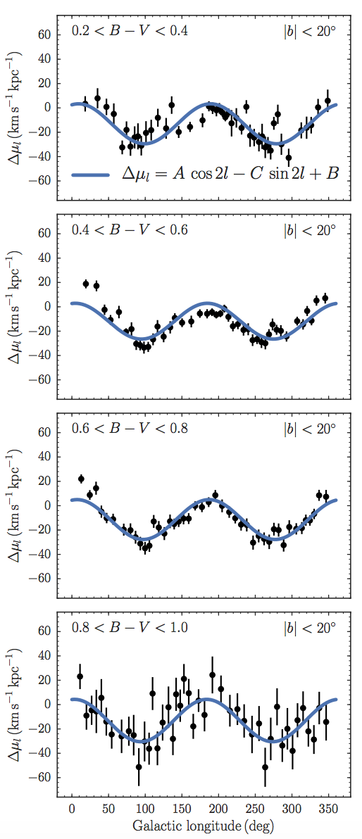
Figure 8.18: Solar-motion-corrected proper motion \(\Delta \mu_l\) versus longitude for stars near the Sun (Bovy 2017a).
This figure beautifully displays the dominant \(\cos 2l\) behavior expected from Equation (8.29) for a close-to-axisymmetric disk (\(C \approx 0\) and therefore the \(\sin 2l\) term is sub-dominant). The overall offset from zero is \(B\). From these figures it should be clear that \(A \approx -B \approx 15\,\mathrm{km\,s}^{-1}\,\mathrm{kpc}^{-1}\). A detailed fit gives \begin{align}\label{eq-galrot-obsOort-A} A & = \phantom{-}15.3 \pm 0.4 \,\mathrm{km\,s}^{-1}\,\mathrm{kpc}^{-1}\,; \quad B = -11.9 \pm 0.4 \,\mathrm{km\,s}^{-1}\,\mathrm{kpc}^{-1}\,;\\ C & = -\phantom{1}3.2 \pm 0.4\,\mathrm{km\,s}^{-1}\,\mathrm{kpc}^{-1}\,;\quad K = -\phantom{1}3.3\pm 0.6\,\mathrm{km\,s}^{-1}\,\mathrm{kpc}^{-1}\,.\label{eq-galrot-obsOort-K} \end{align} All of these were determined from observations of the proper motions alone. This makes use of the fact that if we assume that the disk is in cylindrical rotation, then Equation (8.28) applies to the component of the line-of-sight velocity that is parallel to the mid-plane. But for \(b \neq 0\), the actual line-of-sight velocity is directed away from the mid-plane, and the cylindrical radial velocity gets mixed into the line-of-sight velocity as well as the \(b\) component of the proper motion in the observational spherical coordinate system. This leads to an equation for \(\mu_b(l)\) similar to Equation (8.29) \begin{align} \mu_b(D,l) = &- \left( K + A\,\sin 2l + C\,\cos 2l\right)\,\sin b\,\cos b\nonumber\\&+\frac{1}{D}\left[\left(U_0\,\cos l + V_0\,\sin l\right)\,\sin b - W_0 \cos b\right]\,,\label{eq-oort-pmb-b} \end{align} where we have now explicitly included the \(b\) dependence and \(W_0\) is the Sun’s motion vertically with respect to the plane. Therefore, we can use observations of \(\mu_b(l)\) to determine \(A\), \(C\), and \(K\) and combine them with the \(A\), \(B\), and \(C\) measurements from \(\mu_l(l)\) to determine all four Oort constants. For completeness and for use in Chapter 10, we also state the equations for \(v_\mathrm{los}(D,l)\) and \(\mu_l(D,l)\) that include the \(b\) dependence \begin{align}\label{eq-oort-vlos-b} v_\mathrm{los}(D,l) & = D\,\left[K + A\,\sin 2l + C\,\cos 2l\right]\,\cos b-\left(U_0\,\cos l + V_0\,\sin l\right)\cos b + W_0\,\sin b\,,\\ \mu_l(D,l) & = \left(B + A\,\cos 2l - C\,\sin 2l\right)\,\cos b+\frac{1}{D}\left[U_0\,\sin l - V_0\,\cos l\right]\,.\label{eq-oort-pm-b} \end{align}
The measurements of the Oort constants indicate that (i) the rotation curve is slightly declining at the Solar circle, with \(\mathrm{d}v_c(R) / \mathrm{d} R \approx -3\,\mathrm{km\,s}^{-1}\,\mathrm{kpc}^{-1}\), (ii) the angular rotation rate is \(\Omega(R_0) \approx 27\,\mathrm{km\,s}^{-1}\,\mathrm{kpc}^{-1}\), in good agreement with the standard values of \(v_c(R_0) = 220\,\mathrm{km\,s}^{-1}\) and \(R_0 = 8\,\mathrm{kpc}\), which give \(v_c(R_0) / R_0 = 27.5\,\mathrm{km\,s}^{-1}\,\mathrm{kpc}^{-1}\), and (iii) the disk is non-axisymmetric because both \(C\) and \(K\) are significantly different from zero; however, non-axisymmetry can be largely treated as a perturbation near the Sun, because \(|C|/(A-B)\) and \(|K|/(A-B) \ll 1\).
To interpret the measurements discussed here in terms of the rotation curve, we have assumed that the observed stars on average travel on circular (or at least closed in the case of non-axisymmetry) orbits. We will see in Chapter 10 that this is in fact not the case: In typical disks, the average rotation velocity of a sample of stars at a given radius is less than the circular velocity at that radius. However, the effect of this on the Oort constants \(A\) and \(B\) is small—less than \(\approx 1\,\mathrm{km\,s}^{-1}\,\mathrm{kpc}^{-1}\) (Bovy 2015)—so the mean-field kinematics of nearby stars provides rather accurate measurements of the Oort constants and Galactic rotation in the Milky Way.

 .
. .
. .
.