
15. Gravitational lensing
So far in this book, we have only used the motions of stars, gas, and entire stellar clusters or galaxies to infer the mass distributions of galactic systems. But there are a variety of other methods in use to determine stellar and total masses of galaxies and one of the most useful, assumption-free, and frankly fascinating ones, is gravitational lensing. The field of gravitational lensing is built on the fact that light in a gravitational field gets deflected from its otherwise straight trajectory and that mass distributions therefore act like an optical lens on light. Because the amount of deflection light experiences, as well as the more complex lensing phenomenology, depends only on the instantaneous distribution of total mass, gravitational lensing is a valuable tool to determine the mass distribution within galaxies, clusters of galaxies, and of the Universe as a whole. A taste of the wondrous phenomena that gravitational lensing gives rise to is given in Figure 15.1 :
|
|
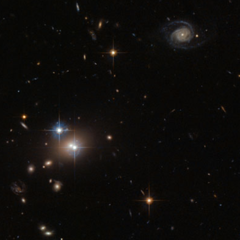
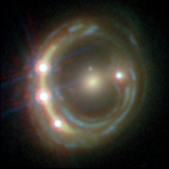
Figure 15.1: Gravitational lenses. Left: QSO 0957+561, the “Twin quasar” (the two bright points straddling the galaxy in the bottom-left quadrant of the image; NASA/ESA Hubble Space telescope). Right: RXJ1131-1231 (NASA/ESA Hubble Space telescope and Suyu et al. 2017).
the left image shows the first discovered gravitational lens, the “twin quasar” QSO 0957+561 (Walsh et al. 1979) and the right image is the quadruply-imaged quasar RXJ1131-1231, whose four quasar images are embedded in an Einstein ring resulting from the lensing of the quasar’s host galaxy (Sluse et al. 2003).
Soldner (1804) first discussed the deflection of light by massive objects. He considered light to be a particle on a hyperbolic orbit around a central mass (e.g., the Sun); because the mass \(m\) of a particle does not affect its orbit in a potential with mass \(M\) as long as \(m \ll M\), the mass of the particle drops out and the deflection angle for light can be estimated. This Newtonian deflection can be easily computed using the method that we used in Chapter 5.1 to calculate the velocity change \(\delta v_y\) of a particle moving along the \(x\) axis that passes by a massive body with mass \(M\) with impact parameter \(b\): the deflection is \(\hat{\alpha} = \delta v_y / v = 2GM/(bc^2)\) for a particle moving at the speed of light \(v=c\) (Equation 5.3). This calculation assumes that gravity bends light and there was no reason to believe that this was the case in the Newtonian theory of light. Einstein (1911) demonstrated from the equivalence principle, which would form the foundation of the general theory of relativity (GR), that gravitational fields have to bend light; working without the full GR field and geodesic equations, he obtained the same result \(\hat{\alpha} = 2GM/(bc^2)\). Soldner (1804) ends his paper by stating “Hopefully no one finds it problematic, that I treat a light ray almost as a ponderable body” (translation by Wikisource). And indeed, with the full set of GR equations, Einstein showed that this was problematic: GR in fact predicts a deflection that is twice as big: \(\hat{\alpha} = 4GM/(bc^2)\) in the case of a central mass (Einstein 1916; see below).
While Einstein’s general theory of relativity had already successfully postdicted the anomalous precession of Mercury (which amounts to \(43''\); Le Verrier 1859; Newcomb 1882) as resulting from a first-order correction to the gravitational force coming from the Sun, Einstein’s prediction that light deflection in GR is twice the Newtonian prediction allowed for the first real test of GR. For a light ray grazing the surface of the Sun, the Newtonian and GR predictions are respectively \(0''.875\) and \(1''.75\), predictions that could be distinguished by observations at the time. The eclipse of 1919 presented the first opportunity to test GR in this way (Eddington 1919) and, as is well known now, the observations confirmed the GR prediction, marking the triumph of GR over Newtonian gravity (Dyson et al. 1920; modern measurements confirm the GR prediction and rule out the Newtonian deflection by \(\gtrsim 600\) times the error, e.g., Lebach et al. 1995).
With the fact that gravity bends light rays now established, astrophysicists started considering additional effects that could result from this action. Eddington (1920) and Chwolson (1924) pointed out that gravitational lensing could result in the light from distant objects having multiple light paths towards us, which would give rise to multiple images separated by small angles, so-called image splittings. Einstein (1936) considered the gravitational lensing effect of a star on a background star, but concluded that the micro-arcsecond image splittings are too small to be observed. But the first to propose that gravitational lensing could become the essential tool in extragalactic astronomy that it has become in the last decades was Zwicky (1937a). Based on his determination that the dynamical mass of the Coma cluster estimated using the virial theorem was hundreds of times larger than previously assumed based on the light coming from Coma-cluster galaxies (Zwicky 1933; see Chapter 6.1), he found that galaxies are massive enough to produce image splittings of background sources with separations \(\approx 1''\). Zwicky (1937b) further calculated that the probability of this lensing effect is \(\approx 1\%\), a prediction that has held up remarkably well over the years: gravitational lensing by galaxies is therefore a rare, but not impossible phenomenon to observe.
Nevertheless, it took another few decades to observe the first gravitational lens, largely due to the lack of bright objects that can be seen over the cosmological scales necessary to have a good chance of experiencing gravitational lensing. The discovery of quasars as bright extragalactic sources in the 1960s (see Chapter 18.3), however, cleared the path towards discovery, because quasars are both bright enough that they could be seen to cosmological distances, and rare enough that seeing identical quasars within a few arcseconds is too much of a coincidence to explain without gravitational lensing. The first gravitationally-lensed quasar was discovered by Walsh et al. (1979) and is known as the “twin quasar” (QSO 0957+561; see Figure 15.1). It was soon followed by other multiply-imaged quasars, including some with more than two images (e.g., Weymann et al. 1980; Young et al. 1981; Huchra et al. 1985), the discovery of background galaxies lensed into arcs by clusters of galaxies (Lynds & Petrosian 1989; Soucail et al. 1987), and the discovery of Einstein rings formed by the gravitational lensing of compact radio galaxies (Hewitt et al. 1988). Today, hundreds of lensed quasars and galaxies are known, with large numbers added recently from large photometric and spectroscopic surveys (e.g., Canameras et al. 2020; Huang et al. 2021). The LSST survey on the Vera Rubin Observatory and other upcoming surveys should soon increase this to tens of thousands of lensed quasars. Multiple or strongly-deformed images are the hallmark of strong lensing, but it was also quickly realized that the smaller effect from lensing further from the centers of massive galaxies and clusters could be detected statistically through correlated changes in the shapes of background galaxies. This regime is known as weak lensing and it was first discovered in massive clusters acting as lenses of a population of faint, blue background galaxies (Tyson et al. 1990). Because weak lensing can probe the mass distribution far from galaxies’ centers, it is especially useful for measuring the total dark matter masses of galaxies (e.g., Brainerd et al. 1996). Similarly, the combined effect of all intervening mass in the Universe causes a general distortion of observed galaxies that can be used to determine the energy content of the Universe (Kristian & Sachs 1966). This cosmic shear effect has become one of the major cosmological probes since its first measurement (Wittman et al. 2000; Abbott et al. 2018). It is clear that gravitational lensing has flourished into a large area of extragalactic astronomy with many exciting discoveries and applications yet to come.
Gravitational lensing has many applications, some of which we will discuss in this and the next chapter. It can be used to study the mass distribution of the lens in a manner that is in many ways orthogonal to the usual dynamical methods (which typically assume equilibrium, which gravitational lensing does not require); both the large-scale (dark matter) and small-scale (stellar) distribution can be studied using different lensing observables. That the lensing effect also includes an overall magnification of the lensed source means that we can use gravitational lensing to study sources that are otherwise too faint, both in our own Galaxy (e.g., Bensby et al. 2013) and at cosmological distances (Zheng et al. 2012). But gravitational lensing is not just a static phenomenon and the time dependence of lensing also has important applications. For example, the gravitational time delay that accompanies lensing (see below) allows lensing to measure the Hubble constant (Refsdal 1964) and the micro-arcsecond lensing (“microlensing”) produced by moving star lenses can be used to study the distribution of stars and compact objects in our own Galaxy (Paczynski 1986b) and in external lens galaxies (Chang & Refsdal 1979).
In this chapter, we give an introduction to the mathematical framework that describes gravitational lensing in its various forms. We discuss in some detail how gravitational lensing is used to constrain the mass distributions of galaxies and clusters of galaxies, but discuss results derived from gravitational lensing on the mass distribution and structure of galaxies in more detail in the next chapter. While the cosmic-shear lensing effect of the entire large-scale mass distribution of the Universe has become an important cosmological probe, we focus on lensing by individual stars, galaxies, and clusters of galaxies here and do not discuss the somewhat different formalism necessary to study cosmic shear.

 .
. .
. .
.