
8.1. Velocity fields in external galaxies
8.1.1. A very brief overview of the observations
Observations of the interstellar medium in external galaxies consist of measurements of emission-line spectra over a one-dimensional or two-dimensional locus in the sky covering the galaxy. The Doppler shifts of the observed lines contain information about the line-of-sight kinematics of the galaxy. Typical lines that are used are H\(\alpha\) at \(6564.614\AA\) and [NII] at \(6585.27\AA\) (these are vacuum wavelengths), those of CO in the millimeter region, and the 21cm line of neutral hydrogen that results from spin flips between the atom’s electron and proton. One should match the observed spectral range such that all velocities that are plausibly associated with the observed galaxy produce Doppler shifts that fall within the observed range. The observed spectrum in principle maps the entire line-of-sight velocity distribution onto wavelength, but in this chapter we will use only the mean velocity field \(V(x,y)\) at a given position \((x,y)\) on the sky. Unless stated otherwise, the Cartesian system \((x,y)\) will be defined galaxy-by-galaxy such that (i) the center of the light is at \((0,0)\), (ii) the galaxy’s major axis lies at \(y=0\), and (iii) the peak recession velocity lies at positive \(x\) at \(y=0\) (we will assume that the kinematic major axis coincides with the photometric major axis, although this does not need to be the case in the presence of non-axisymmetric motions). Comparisons between the observed line profile and the line profile of a line at a single velocity allow one to measure the velocity dispersion and even higher order moments of the velocity distribution, but these require very good data.
Traditionally, optical measurements are made with a long-slit spectrograph, which produces a one-dimensional trace. For reasons that will become clear below, this one-dimensional locus is best placed along the major axis (\(y=0\)) and these observations therefore produce \(V(x,0)\) in the notation above. A typical example are the velocity fields observed by Rubin et al. (1980) shown in Figure 8.1.
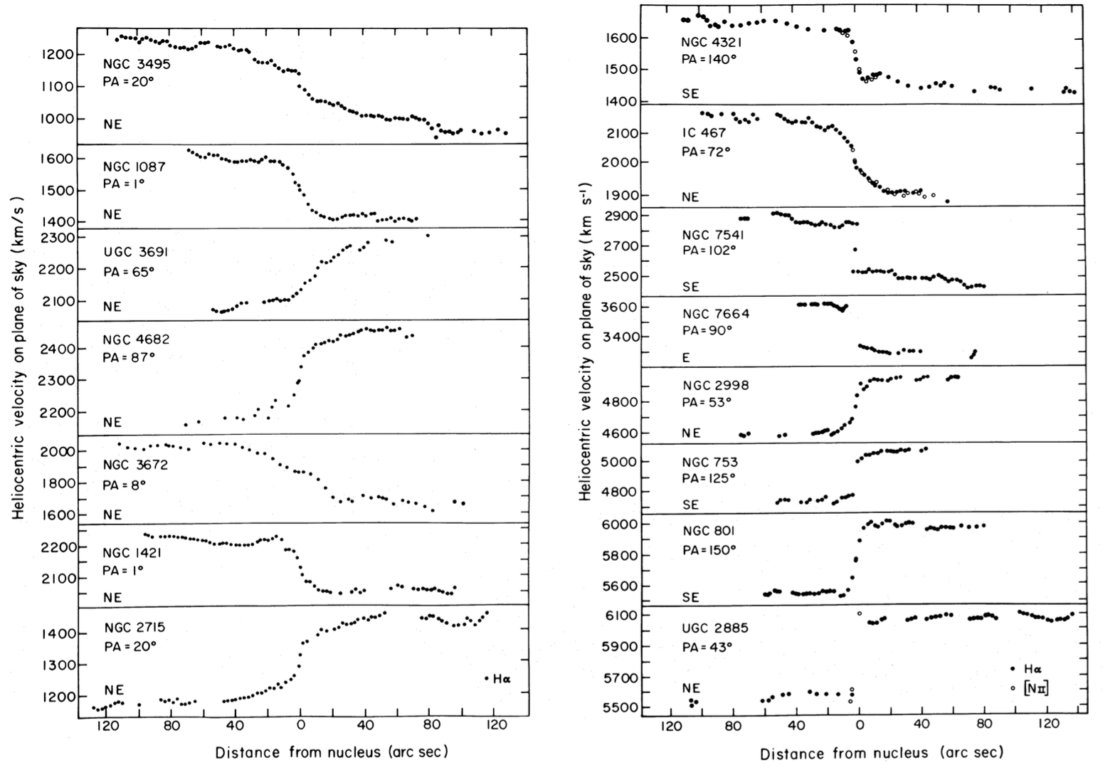
Figure 8.1: Velocity fields along the major axis (Rubin et al. 1980).
Integral-field observations now also routinely provide the full \(V(x,y)\) for optical emission lines (e.g., CALIFA: Sánchez et al. 2012; MaNGA: Bundy et al. 2015; SAMI: Croom et al. 2012).
CO and radio 21cm observations typically provide the two-dimensional velocity field \(V(x,y)\). A canonical example are the velocity fields of 22 spiral galaxies observed as part of Albert Bosma’s famous doctoral dissertation, displayed in Figure 8.2.
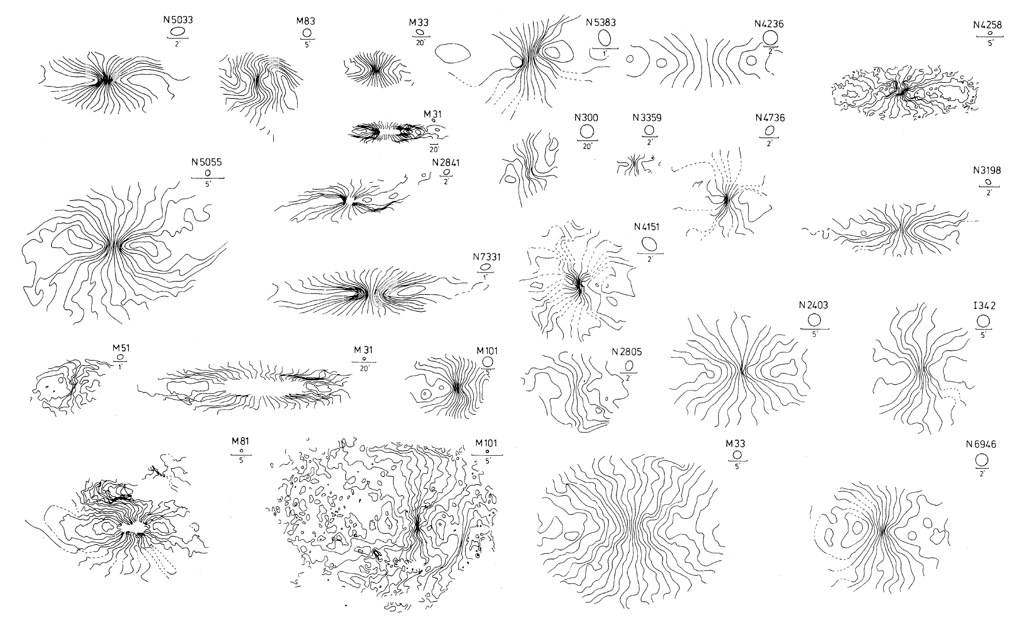
Figure 8.2: Two-dimensional velocity fields from 21 cm observations (Bosma 1978).
This figure shows contours of constant velocity and these velocity fields have all been oriented such that the major axis is horizontal for each galaxy. The velocity fields display all of the major types of features that one sees in two-dimensional velocity fields: (i) regions of vertical contours of constant velocities near the center, (ii) the spider-like shape of contours extending radially from the center, and (iii) closed contours along the major axis away from the center. We will discuss how all of these result from different types of galactic rotation and how we can essentially directly read off the rotation curve of these galaxies from these diagrams.
Two-dimensional velocity fields contain much more information than one-dimensional slices through them. In particular, they allow us to see deviations from circular rotation and from simple galactic geometry (for example, if the kinematic and photometric major axes do not coincide). Two-dimensional velocity fields are therefore essential to determining the best possible representation of a galaxy’s rotation curve, which we can define as follows: the velocity a test particle would have if it was on a circular orbit in an axially-symmetrized version of a galaxy’s mass distribution. By “axially-symmetrized” here we mean the galaxy’s mass distribution at radius \(R\) averaged around the axis perpendicular to the disk (this averages over, e.g., spiral structure’s deviations). We will discuss how we can determine a galaxy’s rotation curve from observations of its velocity field in Section 8.2.1 below.
Velocity fields remain one of the basic tools to learn about galactic structure, so before continuing with a detailed discussion of what they teach us about galactic rotation, we will look at a few more examples. Figure 8.3 shows a study of the galaxy NGC 3198 from the THINGS survey (Walter et al. 2008).
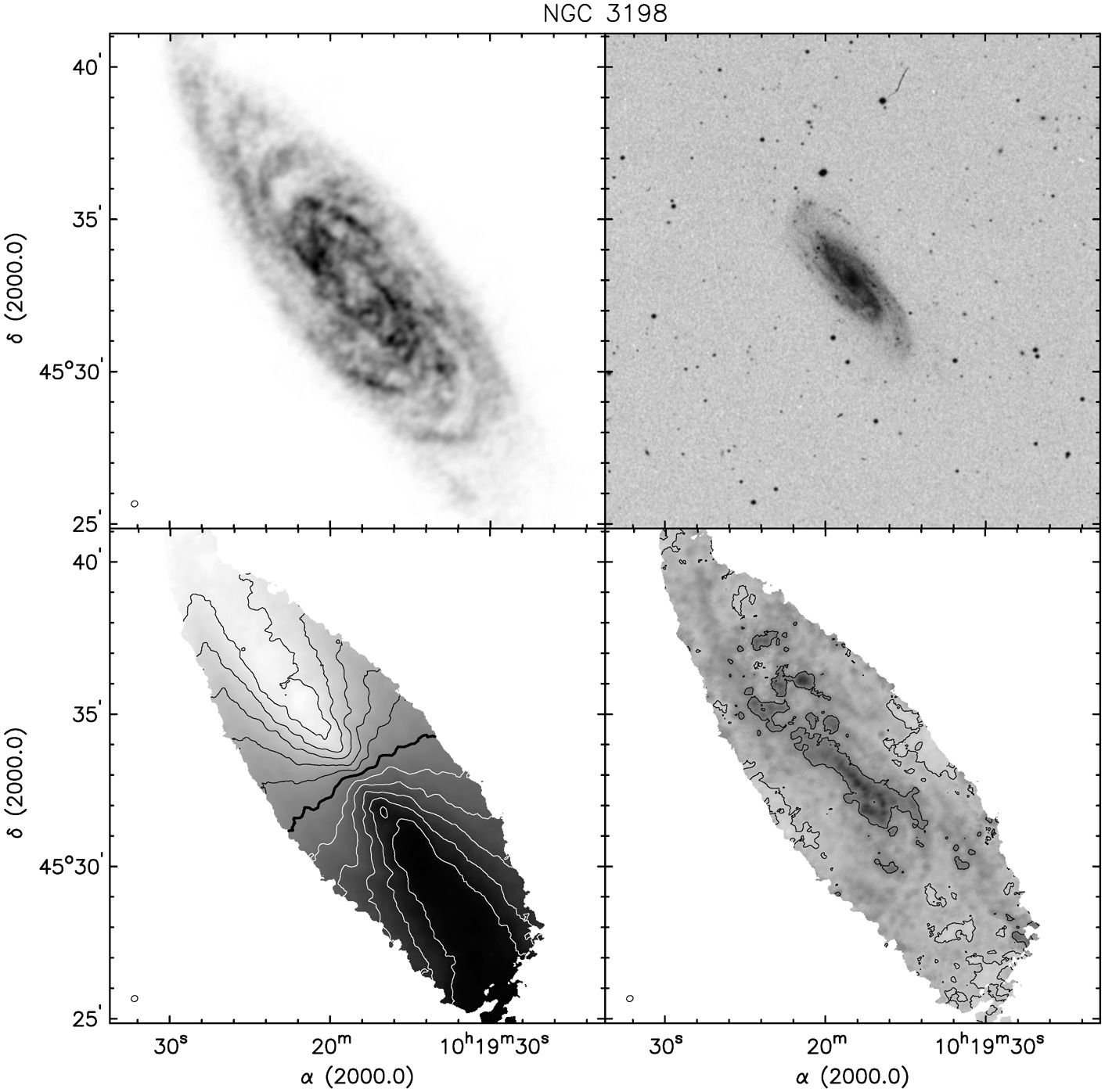
Figure 8.3: Structure and kinematics of NGC 3198: HI emission (top, left), optical emission (top, right), HI mean velocity field (bottom, left), and HI velocity dispersion (bottom, right) from the THINGS survey (Walter et al. 2008).
NGC 3198 is a galaxy famous for its rotation curve. After reading the next section, you should be able to immediately pinpoint why from the lower-left image. The observations extend out to about 40 kpc from the center and darker grayscale indicates receding velocities.
As a final example, through the use of adaptive-optics-guided spectrographs, we can now observe velocity fields of lines such as H\(\alpha\) for redshifts of one to three, allowing us to study galactic rotation and structure at earlier times in the Universe. For example, Figure 8.4 shows velocity fields for a selection of galaxies in the SINS H\(\alpha\) sample at redshifts in the range of one to three (Förster Schreiber et al. 2009).
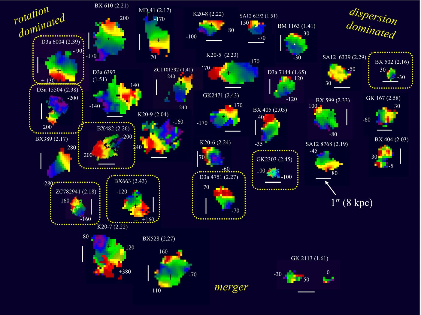
Figure 8.4: Velocity fields of galaxies at \(z \approx 2\) (Förster Schreiber et al. 2009).
With such H\(\alpha\) velocity fields being measured for more and more high-redshift galaxies, and with similar observations now possible for CO using the Northern Extended Millimeter Array (NOEMA; e.g., Uebler et al. 2018) and the Atacama Large Millimeter/submillimeter Array (ALMA), and with the coming resurgence of HI velocity fields from the Square Kilometer Array (SKA) and its precursors, the interpretation of velocity fields therefore remains as important as ever.
8.1.2. Velocity fields of axisymmetric disk galaxies
To model galactic velocity fields, we consider a disk in circular rotation with rotation curve \(v_c(R)\), observed from our location. We will assume that the systemic velocity with respect to us is zero, because it simply adds a constant to all observed velocities. A location at radius \(R\) in the galaxy will have a velocity \(\vec{v} = -v_c(R)\,(\vec{\hat{R}}\times\vec{\hat{n}})\), where \(\vec{\hat{R}}\) is the unit vector that points to the location from the galaxy’s center and \(\vec{\hat{n}}\) is a unit vector normal to the disk plane. The observed line-of-sight velocity \(V\) is then the dot product of the velocity \(\vec{v}\) and the direction of the line-of-sight, \(\vec{\hat{r}}\), pointing from us to the galaxy: \begin{align} V & = \vec{\hat{r}}\cdot\vec{v}= v_c(R)\,\vec{\hat{R}}\,\cdot\left(\vec{\hat{r}}\times\vec{\hat{n}}\right)= v_c(R)\,\vec{\hat{R}}\,\cdot\vec{\hat{k}}\,\sin i\label{eq-vlos-in-vfield}\,, \end{align} where we have used that \(\vec{a}\cdot(\vec{b}\times\vec{c}) = -\vec{b}\cdot(\vec{a}\times\vec{c})\); \(i\) is the galaxy’s inclination (defined such that an an edge-on galaxy has an inclination of \(i=90^\circ\)) and \(\vec{\hat{k}} = (\vec{\hat{r}}\times\vec{\hat{n}})/\sin i\) is the unit vector perpendicular to both \(\vec{\hat{r}}\) and \(\vec{\hat{n}}\).
Now we introduce a pair of two-dimensional coordinate systems. The first Cartesian system \((x,y)\) is a system on the plane of the sky: we define the center such that the center of the galaxy is at \((x,y) = (0,0)\) and we orient the galaxy such that the intersection between the sky plane and the plane of the disk—the line of nodes—lies at \(y=0\); this is the major axis of the galaxy’s projection onto the sky. We will denote polar coordinates in this system as \((r,\phi)\). Then the projection of \(\vec{\hat{k}}\) points along \((1,0)\). The second coordinate system is in the plane of the galaxy and we will typically only consider polar coordinates \((R,\theta)\) for this system, but denote the Cartesian coordinates as \((x',y')\) when we need them. The vector \(\vec{\hat{k}}\) lies in this plane and has (Cartesian) components \((1,0)\); \(\vec{\hat{R}}\) also falls in this plane and has Cartesian components \((\cos\theta,\sin\theta)\). Then Equation (8.1) becomes \begin{equation}\label{eq-twovfield-axi} V(x,y) = v_c(R)\,\cos\theta\,\sin i\,. \end{equation} When we need to include a systemic velocity of the entire galaxy with respect to the observer, this simply adds a constant \(V_0\) to the left-hand side.
From the definition of the coordinate systems, we can derive a few useful relations between coordinates in the sky plane and those in the galaxy plane. We have that \begin{align} x' & = x\,;\quad y' = \frac{y}{\cos i}\,, \end{align} and \begin{equation} \tan \theta = \frac{\tan \phi}{\cos i}\,. \end{equation}
Equation (8.2) immediately makes it clear why when one is limited to observing a one-dimensional slice of the two-dimensional velocity field using long-slit spectroscopy, it is advantageous to observe along the major axis: \(\theta = 0\) or \(180^\circ\) there and we therefore have \(V(x,0) = \mathrm{sign(x)}\,v_c(R)\,\sin i\), the maximum observed velocity of any \(\theta\). Thus, the velocity along the major axis is simply the rotation velocity \(v_c(R)\) multiplied by the sine of the inclination. This produces the (reversed) S-shape behavior in Figure 8.1 above. But the mapping \(v_c(R) = V(x,0)/\sin i\) assumes that non-circular motions are unimportant.
To gain a better understanding of the observed velocity fields, we now look at a few simple examples.
8.1.3. Solid-body rotation
As discussed in Chapter 2.4.2, a homogeneous density distribution produces solid-body rotation with \(\Omega = v_c(R) / R = \mathrm{constant}\). If we plug this into Equation (8.2) we get \begin{equation} V(x,y) = \Omega\,R\,\cos\theta\,\sin i\,. \end{equation} Because, \(x = x' = R\cos\theta\), this becomes simply \begin{equation} V(x,y) = \Omega\,x\,\sin i\,. \end{equation} The velocity therefore does not depend on \(y\) and contours of constant velocity will run parallel to the \(y\) axis. When we see vertical contours of constant velocity near the center of a two-dimensional velocity field, this is indicative of solid-body rotation. This is often observed in the velocity fields of external galaxies, for example, in Figure 8.2 above.
8.1.4. A flat rotation curve
When we have a flat rotation curve, \(v_c(R) = v_c = \mathrm{constant}\), Equation (8.2) becomes \begin{align} V(x,y) & = v_c\,\cos\theta\,\sin i= v_c\,\frac{x}{R}\,\sin i= v_c\,\frac{\sin i\,\cos i}{\sqrt{\cos^2 i+\tan^2 \phi}}\,. \end{align} Because the observed velocity only depends on \(\tan \phi\), it only depends on \(y/x\) and the contours of equal velocity are straight lines through the center. Thus, when we see regions of the two-dimensional velocity field of galaxies where the contours are straight lines pointing away from the center, this indicates that the rotation curve is flat in those regions.
8.1.5. A peaked rotation curve
Finally, we consider what happens when the rotation curve of a galaxy rises to a maximum value and then declines. We write Equation (8.2) as \begin{equation} V(x,y) = v_c(R)\,\sin i\,\frac{x}{R}\,. \end{equation} Along the \(y=0\), positive \(x\) locus, \(V(x,0) = v_c(R)\,\sin i\). When there are two different \(R_1\) and \(R_2\) at which a certain value of \(v_c\) is reached—one at a radius before the peak of the rotation curve, one after—this means that the value \(v_c\,\sin i\) is reached at two values along the \(x\) axis: at \(R_1\) and at \(R_2\). Similarly, along the same contour at fixed \(y\neq 0\), the same value \(V(x,y) = v_c(R_1)\,\sin i\) will be reached at two different \(x\), because if \(V(x_1,y)\) lies along the contours, then so does \(V(x_1\,R'_2/R'_1,y)\) where \(V(x_1\,R'_2/R'_1,y) = v_c(R'_1)\,\sin i\,x_1/R'_1\) and \(v_c(R'_1) = v_c(R'_2)\). Because \(x/R \leq 1\), if we follow a constant \(V\) contour starting at \(y=0\) upwards, it has to curve towards the \(x\) value at which the rotation curve peaks, because \(v_c(R)\) needs to increase to balance the decrease in \(x/R\) and maintain a constant \(V\). The contour keeps growing towards larger \(y\) until the required \(v_c(R)\) is the maximum value of the circular velocity. Then the contour turns down to decreasing \(y\) again until reaching the second value along \(y=0\) where the velocity is \(V\). The same happens when continuing down to negative \(y\) and all contours corresponding to \(V(x,0) = v_c(R)\,\sin i\) for \(v_c(R)\) that exist before and after the radius of maximum \(v_c\) therefore close.
Thus, if we see a closed contour in the two-dimensional velocity field \(V(x,y)\) of a galaxy, this means that the rotation curve reaches a maximum. Because for an isolated galaxy we assume that \(v_c(0) = v_c(\infty) = 0\), all contours should eventually close. But if the rotation curve does not decline within the observed area, then we may not see contours close within the observed area. And a single galaxy is of course not the only thing in the Universe, so practically a contour will not close if the circular velocity curve remains high into the surrounding environment.
In the velocity fields of Bosma (1978) from Figure 8.2 and in that of NGC 3198 from Figure 8.3, we see that the contours do not close for many of the observed galaxies, even though they extend out to dozens of kpc. Disk galaxies have light distributions that are observed to be exponential (Chapter 7.1) and if we assign a constant mass-to-light ratio to these galaxies, then the mass distribution should be that of an exponential disk. We computed the rotation curve for the exponential disk in Chapter 7.3.3.2 and found that it peaks at \(R \approx 2.15\,R_d\). Because galaxies have scale lengths \(R_d\) of a few kpc typically, we would therefore expect their rotation curves to peak at \(R \approx 10\,\mathrm{kpc}\) if their mass-to-light ratios are constant. Thus, we should see that contours in the velocity field start to close around \(R \approx 10\,\mathrm{kpc}\), but this is not what is observed.
8.1.6. Comparing different models and the cored logarithmic potential
Figure 8.5 summarizes what we have learned from these three examples. We define a general function that computes and plots the two-dimensional velocity field in for any potential in galpy:
[6]:
from galpy.potential import vcirc
def plot_twod_vfield(pot,sini=0.5,
                     title=None,
                     xmin=-2.,xmax=2.,nxs=100,
                     ymin=-2.,ymax=2.,nys=100,**kwargs):
    Vfield= numpy.empty((nxs,nys))
    xs= numpy.linspace(xmin,xmax,nxs)
    ys= numpy.linspace(ymin,ymax,nys)
    cos2i= 1.-sini**2.
    for ii in range(nxs):
        for jj in range(nys):
            R= numpy.sqrt(xs[ii]**2.+ys[jj]**2./cos2i)
            Vfield[ii,jj]= vcirc(pot,R)*xs[ii]/R*sini
    dx= xs[1]-xs[0]
    dy= ys[1]-ys[0]
    out= galpy_plot.dens2d(Vfield.T,origin='lower',
                           xrange=[xmin-dx/2.,xmax+dx/2.],
                           yrange=[ymin-dy/2.,ymax+dy/2.],
                           xlabel=r'$x$',ylabel=r'$y$',
                          **kwargs)
    if not title is None:
        annotate(title,(0.5,1.075),xycoords='axes fraction',
                 horizontalalignment='center',
                 verticalalignment='top',size=17.)
    return None
Then we apply this function to plot the rotation curve for the case of solid-body rotation, a flat rotation curve, and a rotation curve that peaks. For the latter, we use galpy’s Milky-Way potential model, MWPotential2014 (Bovy 2015), which peaks at \(R\approx0.5\). We use \(\sin i = 0.5\).
[7]:
from galpy import potential
figure(figsize=(14,5))
subplot(1,3,1)
# size R of homogeneous >> considered region
hp= potential.HomogeneousSpherePotential(normalize=1.,R=10.)
plot_twod_vfield(hp,contours=True,cmap='bwr',gcf=True,
                 title=r'$v_c(R) = \Omega\,R$')
subplot(1,3,2)
lp= potential.LogarithmicHaloPotential(normalize=1.)
plot_twod_vfield(lp,contours=True,cmap='bwr',gcf=True,
                 title=r'$v_c(R) = v_c = \mathrm{constant}$')
subplot(1,3,3)
plot_twod_vfield(potential.MWPotential2014,contours=True,cmap='bwr',
                 levels=numpy.linspace(-.5,.5,21),gcf=True,
                 title=r'$\mathrm{peaked}\, v_c(R)$')
tight_layout()

Figure 8.5: Model velocity fields for simple rotation curves.
These velocity fields agree with our theoretical work above: the solid-body rotation curve gives rise to vertical constant-velocity contours, the flat rotation curve gives radial contours, and the peak in the rotation curve in the right panel causes closed contours along the major axis. The rotation curve on the right drops off very slowly beyond the peak, which is why there are only two closed contours in this figure.
To demonstrate the latter point, we compare the velocity field of a Kuzmin disk and that of a razor-thin exponential disk with the same mass and with the same peak radius. We compared the rotation curves for these two models in Figure 7.11, where we found that the exponential disk peaks at a higher value and that it is therefore more peaked. The two-dimensional velocity fields in the left and middle panels of Figure 8.6 display this clearly.
[8]:
figure(figsize=(14,4))
subplot(1,3,1)
kzp= potential.KuzminDiskPotential(amp=10.,a=2.15/numpy.sqrt(2.))
rp= potential.RazorThinExponentialDiskPotential(amp=10./(2.*numpy.pi),hr=1.)
lp= potential.LogarithmicHaloPotential(normalize=1.,core=0.25)
levels= numpy.linspace(-1.,1.,16)
plot_twod_vfield(kzp,contours=True,cmap='bwr',gcf=True,
                xmin=-7.,xmax=7.,ymin=-7.,ymax=7.,levels=levels,
                title=r'$\mathrm{Kuzmin}$')
subplot(1,3,2)
plot_twod_vfield(rp,contours=True,cmap='bwr',gcf=True,
                xmin=-7.,xmax=7.,ymin=-7.,ymax=7.,levels=levels,
                title=r'$\mathrm{Exponential}$')
subplot(1,3,3)
plot_twod_vfield(lp,contours=True,cmap='bwr',gcf=True,
                 levels=numpy.linspace(-0.5,0.5,13),
                 title=r'$\mathrm{Rising\ to\ flat}$');

Figure 8.6: Model velocity fields for disks (left, middle) and for the cored logarithmic potential (right).
The more peaked nature of the exponential-disk’s rotation curve leads to tighter closed contours than in the case of the Kuzmin disk (the contours in Figure 8.6 are at the same level in both panels). Thus, from the tightness of the closed contours in a two-dimensional velocity field (if there are any), we can directly read off how peaked the rotation curve is.
However, as we will discuss in more detail below, two-dimensional velocity fields typically do not have closed contours, indicating that their rotation curves remain flat out to the observed radius (NGC 3198 in Figure 8.3 is a good example of this). In that case, we should see a velocity pattern that corresponds to a rising rotation curve that flattens at a certain radius. A simple model with this behavior is a cored logarithmic potential: \(\Phi(R) = (v^2_0/2) \ln[R_c^2+R^2]\), which has \(v_c(R) = v_0\,R/\sqrt{R^2+R^2_c}\). At \(R \ll R_c\) , this corresponds to solid-body rotation and at \(R \gg R_c\) the rotation curve is flat; this model is therefore a good representation of a rising-to-flat rotation curve. The velocity field of this model with \(R_c = 0.25\) is shown in the right panel of Figure 8.6. The velocity field goes from the vertical-contour behavior of solid-body rotation near \(x=0\) to the radial behavior of a flat rotation curve at larger \(|x|\). This pattern is very close to the pattern observed in many of the two-dimensional velocity field pictured at the beginning of this chapter.

 .
. .
. .
.