
20.2. Bars
We saw above that cold stellar disks are susceptible to a violent instability that re-arranges all of a disk galaxy’s stars into a bar-shaped structure. So it is unsurprising that many disk galaxies have a prominent bar at their centers. Indeed, in light of simulations such as that shown in Figure 20.5, it is perhaps surprising that not all disk galaxies contain strong bars. In this section, we discuss the observational properties of bars and study their orbital structure and dynamical support, before returning to the question of how they form and evolve.
20.2.1. Observations
Bars are common features in present-day disk galaxies. Overall, approximately two-thirds of low-redshift disk galaxies contain a bar-shaped distortion at their centers (Eskridge et al. 2000; Buta et al. 2015), with about half of these qualifying as a strong bar characterized by almost rectangular equidensity contours (e.g., Aguerri et al. 2009; Nair & Abraham 2010; Masters et al. 2011). In the Hubble classification scheme from Chapter 18.3, strong bars are SBs, while weak bars are SABs. In the high-resolution Spitzer Survey of Stellar Structure in Galaxies (S\(^4\)G; Sheth et al. 2010), the bar fraction displays a strong dependence on stellar mass, with the bar fraction peaking at 70% at \(M_* = 3\times 10^9\,M_\odot\) to \(10^{10}\,M_\odot\) and declining first to about 50% at \(M_* = 5\times 10^{8}\,M_\odot\) and \(M_* = 5\times 10^{10}\,M_\odot\), and then to 20% when going a factor of five lower and higher in stellar mass still (Erwin 2018). Bars thus exist in many but not all disk galaxies and their formation and survival is therefore not a given. As such, bars can be useful tracers of the dynamical state of a single galaxy, which has to allow a bar to form and survive, and of the disk galaxy population as a whole.
Bars have flat luminosity profiles with a relatively sharp cut-off at the bar radius in the earlier Hubble disk types and exponential profiles for the later Hubble types (Elmegreen & Elmegreen 1985). The Milky Way’s bar has an exponential profile (e.g., Wegg et al. 2015). Bar sizes are typically a few kpc and scale approximately linearly with the size of the stellar disk; a useful summary is that bars extend about one to two disk scale lengths (Erwin 2018). The face-on shape of bars varies from elliptical to rectangular with axis ratios ranging from 0.2 to 0.6 (ellipticities from 0.4 to 0.8) with a most common value around 0.4 (Gadotti 2011), incidentally also the axis ratio of the Milky Way’s bar (Bovy et al. 2019). The shape of the bar can be represented through an aximuthal decomposition of the light profile into Fourier components (with significant \(m > 2\) components indicating a non-ellipsoidal shape), but they are also often conveniently determined by fitting the surface-brightness profile with contours of the form (Athanassoula et al. 1990) \begin{equation} \left({|x| \over a}\right)^c+\left({|y| \over b}\right)^c = \mathrm{constant}\,, \end{equation} where \(b/a\) is the axis ratio. A value of \(c=2\) indicates a purely-ellipsoidal shape, while \(c > 2\) for more boxy bars. Fitting a single axis ratio and a single value of \(c\) over their entire profile, bars have \(c \approx 2\) to \(3.5\) (Gadotti 2011), but both the axis ratio—which declines outwards—and the shape parameter \(c\) vary with radius (e.g., Athanassoula et al. 1990). The vertical extent of bars is difficult to determine for external galaxies, because we cannot see the vertical profile in the face-on projections necessary to unambiguously detect a bar. But in the Milky Way, the three-dimensional structure of the bar is that of a peanut or “X”, with a wider vertical extent further from the center (Blitz & Spergel 1991; McWilliam & Zoccali 2010) and edge-on observations of disks demonstrate that about 45% of all disk-galaxy bulges have this same shape (Lutticke et al. 2000). It is thus plausible that all relatively strong bars have a peanut shape, a view that is further strengthened through kinematical determinations of the presence of a bar in edge-on galaxies (Bureau & Athanassoula 2005).
Because bars are relatively compact features at the centers of galaxies, detecting them at higher redshifts requires observations with high spatial resolution. Furthermore, the dependence of the bar fraction on stellar mass in the nearby Universe means that one has to be careful in matching samples across redshift when determining the evolution of the bar fraction with time. Early deep observations with the Hubble Space Telescope revealed a strong decrease in the fraction of strongly-barred spirals with redshift (Abraham et al. 1996; Abraham et al. 1999), with the fraction dropping to \(\lesssim 10\%\) at \(z \approx 1\) (Sheth et al. 2008; Melvin et al. 2014). Figure 20.11 summarizes various observational determinations.
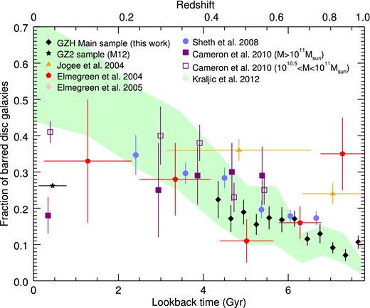
Figure 20.11: The fraction of strongly-barred galaxies as a function of redshift (Melvin et al. 2014).
The strong bar fraction declines by a similar relative amount to the overall bar fraction and strong bars are therefore quite rare at \(z = 1\). The bar fraction in lower-mass galaxies increases faster with time than that in higher-mass galaxies (Cameron et al. 2010). As we saw above, galactic disks form bars when they are relatively cold and have the right dynamical structure, so bar formation occurs when disks reach an ordered, settled state. The decrease of the bar fraction with redshift is therefore consistent with the increase in the fraction of peculiar galaxies with redshift (see Figure 18.18 in Chapter 18.3), with the mass dependence indicating that more massive disks settle down faster than less massive disks.
Bars are not static objects. Because they are essentially straight features, they must rotate with a constant pattern speed across their radial extent, as they would otherwise quickly shear into a spiral pattern. Estimating this pattern speed is possible in various ways, but the most general, robust, and simplest method results from assuming that the density of a tracer of the bar—stars or a gas tracer (but see Williams et al. 2021; Borodina et al. 2023)—on average rotates as the bar and satisfies the continuity equation, that is, that no tracers appear or disappear (e.g., there is no significant contribution from star formation or stellar death). The first assumption implies that the tracer’s surface density is static in a frame rotating at the bar’s pattern speed \(\Omega_b\), that is, \(\Sigma(X,Y,t) \equiv \Sigma(R,\phi-\Omega_b\,t)\). The time derivative of \(\Sigma(X,Y)\) can therefore be written in terms of spatial derivatives and the pattern speed. The continuity equation relates the time derivative of \(\Sigma(X,Y)\) to the spatial divergence of \(\Sigma(X,Y)\,\vec{v}(X,Y)\). Thus, we can relate the pattern speed to spatial derivatives of \(\Sigma(X,Y)\) and \(\Sigma(X,Y)\,\vec{v}(X,Y)\) as follows \begin{align}\label{eq-intevol-bar-continuity} \Omega_b\,\left(Y\,{\partial \Sigma \over \partial X}-X\,{\partial \Sigma \over \partial Y}\right) = {\partial \Sigma \over \partial t} = -{\partial \left(\Sigma\,v_X\right)\over \partial X}-{\partial \left(\Sigma\,v_Y\right)\over \partial Y}\,. \end{align}
In the Milky Way, we can measure the stellar surface density \(\Sigma_*(X,Y)\) in the bar region as well as \(\Sigma_*(X,Y)\,\vec{v}(X,Y)\) and we can thus directly apply this equation to determine the bar’s pattern speed (Bovy et al. 2019); this gives \(\Omega_b = 40\pm2\,\mathrm{km\,s}^{-1}\,\mathrm{kpc}^{-1}\) (Leung et al. 2023). In external galaxies, we cannot measure the full two-dimensional velocity field \(\vec{v}(X,Y)\), but just its projection \(v_{\mathrm{los}}\) onto the line-of-sight, and measuring partial derivatives from observational data is difficult. Thus, in external galaxies one proceeds by integrating Equation (20.64) over the direction parallel to the line of nodes—the \(x\) axis in the notation from Chapter 8.1.2—and then using a weight function \(h(y)\) over the direction perpendicular to the line of nodes, ending up with \begin{equation}\label{eq-intevol-bar-tw} \Omega_b\,\sin i = { \int_{-\infty}^{\infty}\mathrm{d}y\,h(y)\int_{-\infty}^{\infty} \mathrm{d} x \,\Sigma(x,y)\,v_{\mathrm{los}}(x,y) \over \int_{-\infty}^{\infty}\mathrm{d}y\,h(y)\int_{-\infty}^{\infty} \mathrm{d} x \,\Sigma(x,y)\,x}\,, \end{equation} where \(i\) is the galaxy’s inclination. This method is known as the Tremaine-Weinberg method (Tremaine & Weinberg 1984a). Before the advent of integral-field spectroscopy, this method was generally applied to slit-based spectroscopic observations, where \(v_{\mathrm{los}}\) is determined at a single value or a small number of values of \(y\), such that \(h(y) \equiv \delta(y-y_0)\) or \(\sum_i \delta(y-y_{0,i})\) (e.g., Kent 1987; Merrifield & Kuijken 1995; Elmegreen et al. 1996; Debattista et al. 2002), but integral-field spectroscopy allows bar pattern speed determinations using a large number of pseudo-slits covering the bar at different offsets \(y_0\) (e.g., Aguerri et al. 2015; Guo et al. 2019). In practice, in both cases the pattern speed is obtained from a linear fit to the value of the numerator of the right-hand side of Equation (20.65) versus the denominator calculated at different values of \(y_0\). The Tremaine-Weinberg method has allowed for the determination of hundreds of pattern speed measurements in external galaxies (e.g., Géron et al. 2023), which is enough for clear trends to emerge. For example, in the sample of 53 barred galaxies with stellar masses between \(10^{10}\,M_\odot\) and \(3\times 10^{11}\,M_\odot\) from Guo et al. (2019), the mean pattern speed is \(\approx 30\,\mathrm{km\,s}^{-1}\,\mathrm{kpc}^{-1}\) and pattern speeds range from \(\approx 10\,\mathrm{km\,s}^{-1}\,\mathrm{kpc}^{-1}\) to \(\approx 50\,\mathrm{km\,s}^{-1}\,\mathrm{kpc}^{-1}\).
For dynamical reasons that we will discuss below, the natural extent of bars is their corotation radius \(R_{\mathrm{CR}}\), which can be obtained by solving Equation (20.43) for the bar’s pattern speed \(\Omega_b\). For example, in the Milky Way, the bar’s corotation radius is \(\approx 5.5\,\mathrm{kpc}\) (Bovy et al. 2019). The ratio \(\mathcal{R} = R_{\mathrm{CR}} / R_b\) of the corotation radius to the bar radius \(R_b\) parameterizes whether or not a bar extends out to its corotation radius (Elmegreen 1996) and dynamically we expect \(\mathcal{R} > 1\) (Contopoulos 1980; see below). Bars with \(\mathcal{R} \approx 1\) are referred to as fast bars, because they rotate as fast as is dynamically expected; slow bars have \(\mathcal{R} > 1.4\) by convention. The Milky Way has \(\mathcal{R} \approx 1.1\) and bars in external galaxies typically have \(\mathcal{R} = 1.66\pm 0.05\) with a \(1\sigma\) range of \(\mathcal{R} \approx 1\) to \(\mathcal{R} \approx 2.7\) (Géron et al. 2023) and bars thus range from fast to slow; strong bars typically have somewhat smaller \(\mathcal{R}\) than weak bars.
Bars are typically connected to other morphological features in galaxies such as spiral arms. In many strongly-barred spirals, such as NGC 1300 in Figure 1.3, a clear two-armed spiral pattern starts at the ends of the bar; such galaxies are known as SB(s) galaxies. This pattern is typically accompanied by almost straight dust lanes parallel to the bar’s major axis, but slightly offset towards the leading edge of the bar (because spiral arms are almost always trailing features as we will see below, we can use them to determine a galaxy’s rotation direction). NGC 1300 in Figure 1.3 again provides a clear example of this. In other barred galaxies, a thin ring consisting of young, blue stars encircles the bar and spiral structure starts somewhere along this ring, not necessarily at the ends of the bar itself. An example of this SB(r) type of barred galaxy is NGC 2336 shown in Figure 20.12.
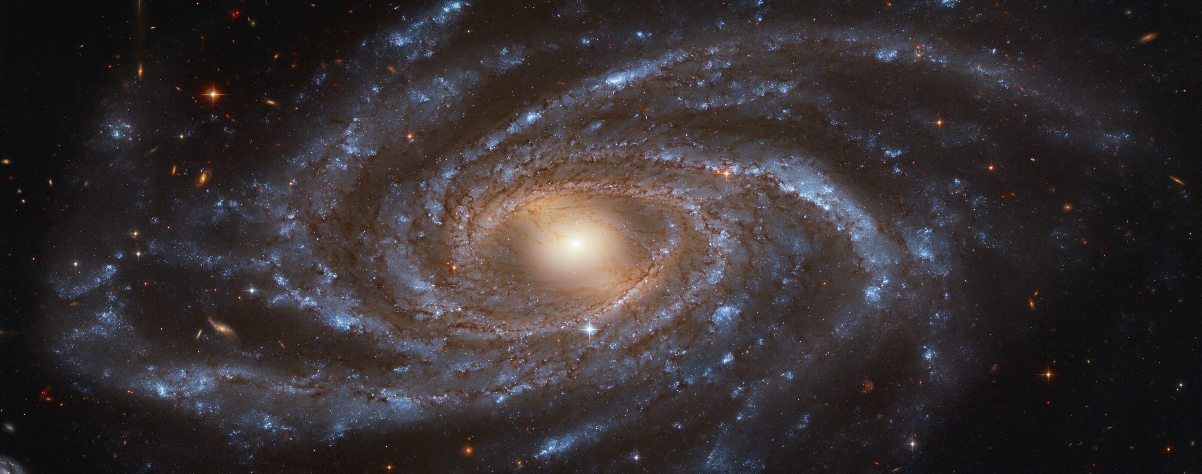
Figure 20.12: NGC 2336, a barred spiral with a ring encircling the bar.
Other barred spirals, such as NGC 4314 shown in Figure 20.1, are intermediate between these two cases and have prominent spiral structure starting near the ends of the bar in conjunction with a ring. The presence of young stars and star-forming gas in the rings encircling bars is in contrast to the mostly quiescent structure of the bar itself, which mainly consists of old stellar populations and has little star formation. Barred galaxies often also have outer rings, with a diameter that is typically about twice the extent of the bar (Kormendy 1979). A prominent example of such an outer ring exists in NGC 1291, shown in Figure 20.13.
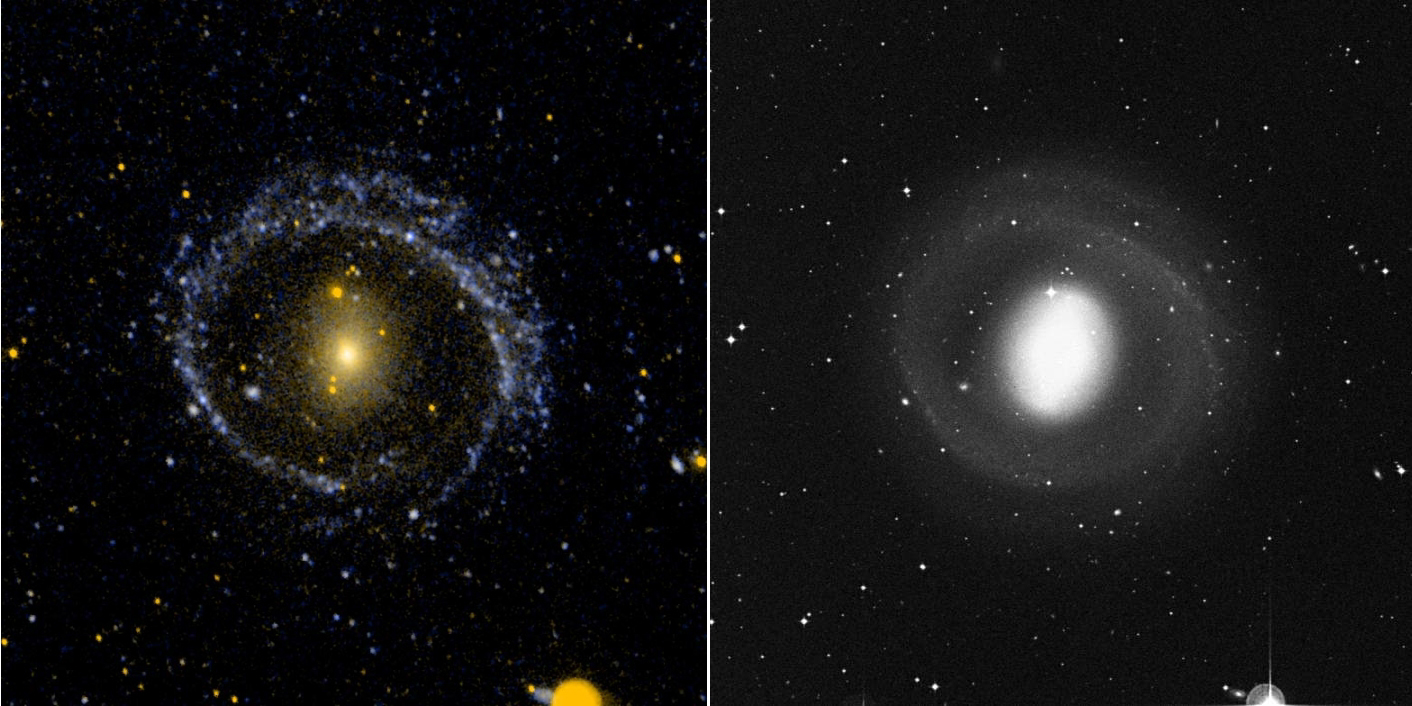
Figure 20.13: NGC 1291, a barred spiral with an outer star-forming ring in visible (right) and ultraviolet (left) light (Credit: NASA/JPL-Caltech/SSC).
The ultraviolet image in the left panel demonstrates that there is vigorous star formation in the outer ring.
As we already saw in NGC 1300 in Figure 1.3, barred spirals often have star-forming nuclear rings as well and, more generally, bars often display strong star formation activity near their centers. This, as well as the prominent dust lanes parallel to the bar’s major axis in SB(s) galaxies is believed to result from bar-driven gas flows to the center, which dynamically are expected to occur at the leading edge of the bar. While spirals typically start at the radius of the bar, whether or not spiral structure in any given galaxy is strongly coupled to the bar remains somewhat unclear, but it appears that it typically is not aside from during episodes of spiral-driven bar growth (Buta et al. 2009). The apparent match between the ends of the bar and the start of two-armed spirals is therefore likely a recurring coincidence in most cases (Sellwood & Sparke 1988).
20.2.2. The orbital structure of bars
As long-lived, massive, triaxial structures, the orbital structure of bars is crucial to determining their formation and long-term fate and to understanding flows of gas into the central regions. One immediate pressing question is what the properties are of self-consistent bars that can exist in galaxies—because bars are often a dominant feature in the galaxies they reside in, their gravitational field must be able to support their three-dimensional density structure self-consistently. This question is the main focus of this and the following section.
As triaxial systems, we are faced with the same issue as in Chapter 13.4, namely that there are not enough integrals of the motion to reduce the six-dimensional phase-space to an easily visualizable form. Thus, similar to Chapter 13.4, we will focus on investigating the orbital structure of two-dimensional bars, which will allow us to understand the in-plane structure of three-dimensional bars that is most important to understanding the dynamics of the bar region. As rotating non-axisymmetric structures, neither the energy nor the \(z\)-component of the angular momentum are conserved in bar potentials. But as long as the bar rotates steadily—and observations give no indication of rapid pattern speed changes that would invalidate this assumption—the Jacobi integral from Equation (19.55) is a conserved quantity that acts much like the specific energy in static systems. Because the bar is static in a frame rotating at its pattern speed, we will typically find it easiest to study bar orbits in this rotating frame, which requires us to add the fictitious centrifugal and Coriolis forces from Chapter 19.4.2.1.
20.2.2.1. Orbits in a logarithmic bar potential
As a simple example that is commonly used to illustrate the orbital structure of bars (e.g., Binney & Tremaine 2008; Sellwood 2014), we approximate the combined bar-plus-axisymmetric galaxy as a rotating cored, non-axisymmetric logarithmic potential given by Equation (13.2). In the bar’s rotating reference frame with pattern speed \(\Omega_b\), the full effective potential is given by \begin{equation}\label{eq-nonaxi-logpot-planar-effpot} \Phi_{\mathrm{eff}}(x,y) = \frac{v_c^2}{2}\,\ln\left(x^2+\frac{y^2}{b^2}+R_c^2\right)-{1\over 2}\,\Omega_b^2\,\left(x^2+y^2\right)\,. \end{equation}
We investigated the orbital structure of the non-rotating version of this potential in Chapter 13.2, finding that a large fraction of its orbital space consists of box orbits that are crucial to creating a self-consistent non-axisymmetric shape. An illustrative surface of section is shown in Figure 13.8. Like in the previous literature, we set \(v_c = 1\), \(b = 0.8\), \(R_c = 0.03\), and \(\Omega_b = 1\), giving a corotation radius of \(R_{\mathrm{CR}} = 1 \approx 30\,R_c\) (see Equation 20.43). The bar’s major axis is aligned with the \(x\) axis in the rotating frame. The bar, thus, has a small constant-density core and then a steeply-declining density profile that gives rise to a constant circular velocity curve. Below, we will demonstrate that the orbital structure of more realistic bar models is similar to that of this simple model.
To start our investigation of the orbital structure of the simple bar model, we take a look at the effective potential in the left panel of Figure 20.14.
[6]:
# First we plot the effective potential of the Milky-Way-like model
# from the next section in the right panel, so we can easily compare
# it to the log-bar one from this section
from galpy.potential import (evaluateplanarPotentials,
                             MWPotential2014,
                             SoftenedNeedleBarPotential,
                             NonInertialFrameForce,
                             toPlanarPotential)
def pot_eff(pot,Omegab,x,y):
    R= numpy.sqrt(x**2.+y**2.)
    phi= numpy.arctan2(y,x)
    return evaluateplanarPotentials(pot,R,phi=phi)-Omegab**2.*R**2./2.
# More realistic amp for the MW is 0.15, but this is a *strong* bar
def setup_mwbarmodel(amp=0.5):
    barp= SoftenedNeedleBarPotential(amp=amp,a=0.5,b=0.,c=0.4*0.5,omegab=0.,pa=0.)
    baramp= -numpy.mean(numpy.fabs([barp.Rforce(1.,0.,phi=p)
                                    for p in numpy.linspace(0.,numpy.pi,101)]))
    MWPotential2014wbar= barp\
        +(1.-(baramp-MWPotential2014[0].Rforce(1.,0.))
              /MWPotential2014[1].Rforce(1.,0.))*MWPotential2014[1]\
        +MWPotential2014[2]
    return toPlanarPotential(MWPotential2014wbar)
pot= setup_mwbarmodel()
Omegab= 4./3.
rotframe= NonInertialFrameForce(Omega=Omegab)
figure(figsize=(10,5))
subplot(1,2,2)
xs= numpy.linspace(-1.3,1.3,100)
ys= numpy.linspace(-1.3,1.3,100)
X,Y= numpy.meshgrid(xs,ys)
c= contour(X,Y,pot_eff(pot,Omegab,X,Y),
        levels=[-5.35,-4.95,-4.55,-4.25,-4.,-3.75,-3.5095,-3.46,-3.425,],
        colors='k',linestyles='-')
clabel(c,inline=True, fontsize=8)
xlabel(r'$x$')
annotate(r'$L_1$',xy=(0.925,0),va='center',fontsize=16.)
annotate(r'$L_2$',xy=(-1.075,0),va='center',fontsize=16.)
annotate(r'$L_3$',xy=(0,0),ha='center',va='center',fontsize=16.)
annotate(r'$L_4$',xy=(0,0.75),ha='center',va='center',fontsize=16.)
annotate(r'$L_5$',xy=(0,-0.75),ha='center',va='center',fontsize=16.);
galpy_plot.text(r'$\mathrm{MW{\text -}like\ bar}$',top_left=True,fontsize=18.,
               bbox={'facecolor':'w','alpha':0.8,'edgecolor': 'None'},zorder=10)
# Now the log bar
from galpy.potential import (evaluateplanarPotentials,
                             LogarithmicHaloPotential)
def pot_eff(pot,Omegab,x,y):
    R= numpy.sqrt(x**2.+y**2.)
    phi= numpy.arctan2(y,x)
    return evaluateplanarPotentials(pot,R,phi=phi)-Omegab**2.*R**2./2.
lp= LogarithmicHaloPotential(amp=1.,b=0.8,core=0.03).toPlanar()
Omegab= 1.
subplot(1,2,1)
xs= numpy.linspace(-1.8,1.8,100)
ys= numpy.linspace(-1.8,1.8,100)
X,Y= numpy.meshgrid(xs,ys)
c= contour(X,Y,pot_eff(lp,Omegab,X,Y),
        levels=[-1.5,-1.0,-0.8,-0.6,-0.4997,-0.4,-0.3,-0.2,0.],
        colors='k',linestyles='-')
clabel(c,inline=True, fontsize=8)
xlabel(r'$x$')
ylabel(r'$y$')
annotate(r'$L_1$',xy=(1.075,0),va='center',fontsize=16.)
annotate(r'$L_2$',xy=(-1.275,0),va='center',fontsize=16.)
annotate(r'$L_3$',xy=(0,0),ha='center',va='center',fontsize=16.)
annotate(r'$L_4$',xy=(0,1),ha='center',va='center',fontsize=16.)
annotate(r'$L_5$',xy=(0,-1),ha='center',va='center',fontsize=16.)
galpy_plot.text(r'$\mathrm{Logarithmic\ bar}$',top_left=True,fontsize=18.,
               bbox={'facecolor':'w','alpha':0.8,'edgecolor': 'None'},zorder=10)
tight_layout();

Figure 20.14: The effective potential of a simple bar potential (left) and of a Milky-Way-like bar (right).
This effective potential has a similar structure to the effective potential from Figure 19.19 of two orbiting point masses in their rotating frame of reference. As is the case there, the effective potential has five extrema known as Lagrange points. The Lagrange point \(L_3\) that is crucial to determining the tidal radius for the orbiting point masses is a local minimum in the bar case. The other four Lagrange points all occur near the corotation radius, with saddle points \(L_1\) and \(L_2\), and local maxima \(L_4\) and \(L_5\). The effective potential at \(L_1\) and \(L_2\) is \(\Phi_\mathrm{eff} \approx -0.5\) (the actual value is \(\approx -0.49955\), but below we will simply refer to this as \(-0.5\)). Because orbits must satisfy \(\Phi_{\mathrm{eff}} \leq E_J\), orbits with Jacobi integral \(E_J < -0.5\) within the eye-shaped region between \(L_1\) and \(L_2\) that is centered on \(L_3\) remain confined there for all time, while orbits with \(E_J \geq -0.5\) are free to travel more freely. It is thus clear that orbits with \(E_J < -0.5\) must be the most important for supporting the bar, because they can confined to a region with a similar shape as the bar itself. We will study orbits with \(E_J < -0.5\) in detail below. There are also orbits with \(E_J < -0.5\) outside of the eye-shaped region, but we will not include these in the study below as their contribution to the bar’s density is negligible because they are not bound to the bar region. In the right panel of Figure 20.14, we show the similar effective potential for the Milky-Way-like bar model that we investigate in Section 20.2.2.2 below. We see that this effective potential is qualitatively the same.
To investigate bar-supporting orbits, we create surfaces of section. Unlike for static non-axisymmetric potentials, we cannot use the technique from Chapter 13.1 to create these, which consists of re-writing the orbit integration in terms of an independent variable that takes on a known value on the surface of section, because the new variable does not always monotonically increase with time due to the fictitious forces in the rotating frame. Instead we rely on a brute-force approach that looks for section crossings using a regular orbit integration.
We start by looking at orbits at the edge of the central constant-density region. The surface of section at \(E_J = -3\) is displayed in Figure 20.15.
[7]:
from galpy.potential import (evaluateplanarPotentials,
                             LogarithmicHaloPotential,
                             NonInertialFrameForce)
from galpy.orbit import Orbit
from matplotlib import cm
from scipy import optimize
def pot_eff(pot,Omegab,x,y):
    R= numpy.sqrt(x**2.+y**2.)
    phi= numpy.arctan2(y,x)
    return evaluateplanarPotentials(pot,R,phi=phi)-Omegab**2.*R**2./2.
def orbit_xvxEJ(x,vx,EJ,pot=None,Omegab=0.):
    """Returns Orbit at (x,vx,y=0) with given E_J"""
    return Orbit([x,vx,numpy.sqrt(2.*(EJ-pot_eff(pot,Omegab,x,0.)-vx**2./2.)),0.])
def zvc(x,EJ,pot=None,Omegab=0.):
    """Returns the maximum v_x at this x and this
       energy: the zero-velocity curve"""
    return numpy.sqrt(2.*(EJ-pot_eff(pot,Omegab,x,0.)))
figure(figsize=(9,4),dpi=300)
lp= LogarithmicHaloPotential(amp=1.,b=0.8,core=0.03).toPlanar()
Omegab= 1.
rotframe= NonInertialFrameForce(Omega=Omegab)
EJ= -3.0
minx= optimize.brentq(lambda x: EJ-pot_eff(lp,Omegab,x,0.),-0.002,-0.07)-1e-10
maxx= optimize.brentq(lambda x: EJ-pot_eff(lp,Omegab,x,0.),0.002,0.07)-1e-10
closed= {'loop-retrograde': [-0.0142,0.],
         'loop-prograde': [maxx-5e-5,0.],
         'box': []}
nonclosed= {'loop-retrograde': [[-0.0001,0.],[-0.005,0.],[-0.01,0.],[-0.012,0.]],
            'loop-prograde': [[0.0396,0.0]],
            'box': [[0.038,0.],[0.035,0.],[0.03,0.],[0.025,0.],[0.02,0.],
                    [0.015,0.],[0.01,0.],[0.005,0.]]}
colors= {'loop-retrograde': 'tab:cyan',
         'loop-prograde': 'tab:blue',
         'box': 'tab:orange'}
ts= numpy.linspace(0.,300.,300001)
for orb in closed:
    if not orb == 'box':
        o= orbit_xvxEJ(closed[orb][0],closed[orb][1],EJ,pot=lp,Omegab=Omegab)
        o.plotBruteSOS(ts,lp+rotframe,surface='y',method='dop853_c',
                       gcf=True,overplot=(orb != 'loop-retrograde'),
                       marker='.',mec='none',zorder=2,
                       mfc=colors[orb],
                       xrange=[-0.05,0.05],yrange=[-1.1,1.1],rasterized=True)
    for nonc in nonclosed[orb]:
        o= orbit_xvxEJ(nonc[0],nonc[1],EJ,pot=lp,Omegab=Omegab)
        o.plotBruteSOS(ts,lp+rotframe,surface='y',method='dop853_c',
                       overplot=True,
                       marker='.',mec='none',zorder=2,ms=4.,
                       mfc=colors[orb],rasterized=True)
# Also plot the zero-velocity curve, first find min x at which it exists
xs= numpy.linspace(minx,maxx,20001)
plot(xs,zvc(xs,EJ,pot=lp,Omegab=Omegab),color='k',zorder=0)
plot(xs,-zvc(xs,EJ,pot=lp,Omegab=Omegab),color='k',zorder=1)
galpy_plot.text(rf'$E_J = {EJ}$',top_right=True,size=18.);

Figure 20.15: Surface of section of the cored, non-axisymmetric, rotating logarithmic potential at \(E_J = -3\) at the edge of the constant-density core.
Unlike the surfaces of section that we saw in Chapter 13, this surface of section is not mirror symmetric around \(x=0\), because the rotation of the frame breaks the \(x \rightarrow -x\) symmetry. We see that there are three main major orbit families, with two of them taking up most of the diagram: a family of retrograde loop orbits (cyan), box orbits (orange), and a family of prograde loop orbits (blue, only at the rightmost edge hugging the zero-velocity curve in black). All three families are stable. Bar orbit families are generally discussed using a notation introduced by Contopoulos & Papayannopoulos (1980) (based on Contopoulos & Mertzanides 1977), in which this family of prograde orbits is known as \(\boldsymbol{x_1}\,\mathbf{orbits}\) and the retrograde family consists of \(\boldsymbol{x_4}\,\mathbf{orbits}\) (we will encounter \(x_2\) and \(x_3\) orbits below as well). The notation derives from the solutions \(x = x_i\) of an equation for periodic orbits in bar potentials (Contopoulos 1975). The parent closed orbits of the \(x_1\) and \(x_4\) families are shown in Figure 20.16.
[8]:
figure(figsize=(7,4.5))
ts= numpy.linspace(0.,10.,10001)
labels= [r'$x_1\,(\mathrm{prograde})$',
         r'$x_4\,(\mathrm{retrograde})$']
for ii,orb in enumerate(['loop-prograde','loop-retrograde']):
    o= orbit_xvxEJ(closed[orb][0],closed[orb][1],EJ,pot=lp,Omegab=Omegab)
    o.integrate(ts,lp+rotframe,method='dop853_c')
    subplot(1,2,ii+1)
    gca().set_aspect('equal')
    o.plot(gcf=True,
           xrange=[-0.049,0.049],
           yrange=[-0.0495,0.0495])
    # Plot contour Phi_eff = EJ
    xs= numpy.linspace(-0.05,.05,100)
    ys= numpy.linspace(-0.05,.05,100)
    X,Y= numpy.meshgrid(xs,ys)
    c= contour(X,Y,pot_eff(lp,Omegab,X,Y),
            levels=[EJ],
            colors='k',linestyles='--',linewidths=1.)
    if ii > 0:
        gca().get_yaxis().get_label().set_visible(False)
        gca().yaxis.set_major_formatter(NullFormatter())
    galpy_plot.text(labels[ii],top_left=True,size=24.)
tight_layout();

Figure 20.16: Closed loop orbits in the cored, non-axisymmetric, rotating logarithmic potential at \(E_J = -3\) at the edge of the constant-density core. The dashed contour is the location of \(\Phi_\mathrm{eff}(x,y) = E_J\).
The \(x_1\) prograde closed loop orbit is strongly flattened in the same sense as the bar (recall that the bar’s major axis lies along \(y=0\)) and much more flattened than the region allowed by \(\Phi_{\mathrm{eff}} \leq E_J\), while the \(x_4\) retrograde orbit is less strongly compressed in the direction perpendicular to the bar. Aside from the box orbits close to the prograde loop orbits in the surface of section, the box orbits are typically not very compressed in the \(y\) direction relative to the \(x\) direction and the prograde loop orbits must therefore be the most important orbits for generating a bar-shaped density distribution.
At slightly higher \(E_J\), a new stable orbit family appears. We leave generating the surface of section at \(E_J = -2.5\) as an exercise, but it is similar to the top one in Figure 20.18. In addition to the main orbit families that we encountered at \(E_J = -3\), it contains three new types of orbit: a second stable prograde family, known as \(\boldsymbol{x_2}\,\mathbf{orbits}\), another closed prograde orbit, known as a \(\boldsymbol{x_3}\,\mathbf{orbit}\), and a chaotic orbit. The \(x_3\) orbit is unstable and very difficult to find in the surface of section. The stable closed loop orbits are shown in the left half of Figure 20.17.
[10]:
fig= figure(figsize=(12,8),constrained_layout=True)
gs= fig.add_gridspec(2,4,hspace=0.)
ts= numpy.linspace(0.,10.,10001)
labels= [r'$x_1\,(\mathrm{prograde})$',
         r'$x_2\,(\mathrm{prograde})$',
         r'$x_4\,(\mathrm{retrograde})$']
for ii,orb in enumerate(['loop-prograde','loop-prograde-x2','loop-retrograde']):
    # Closed
    o= orbit_xvxEJ(closed[orb][0],closed[orb][1],EJ,pot=lp,Omegab=Omegab)
    o.integrate(ts,lp+rotframe,method='dop853_c')
    if ii == 0:
        fig.add_subplot(gs[0,:2])
        yrange=[-0.0125,0.0125]
    else:
        fig.add_subplot(gs[1,ii-1])
        yrange=[-0.095,0.095]
        gca().set_aspect('equal')
    o.plot(gcf=True,
           xrange=[-0.085,0.085],
           yrange=yrange)
    if ii == 0:
        gca().get_xaxis().get_label().set_visible(False)
    if ii > 1:
        gca().get_yaxis().get_label().set_visible(False)
        gca().yaxis.set_major_formatter(NullFormatter())
    galpy_plot.text(labels[ii],top_left=True,size=24.)
    # Non-closed
    o= orbit_xvxEJ(nonclosed[orb][-ii-1][0],nonclosed[orb][-ii-1][1],EJ,pot=lp,Omegab=Omegab)
    o.integrate(ts,lp+rotframe,method='dop853_c')
    if ii == 0:
        fig.add_subplot(gs[0,2:])
        yrange=[-0.0125,0.0125]
    else:
        fig.add_subplot(gs[1,ii+1])
        yrange=[-0.095,0.095]
        gca().set_aspect('equal')
    o.plot(gcf=True,lw=.5,
           xrange=[-0.085,0.085],
           yrange=yrange)
    if ii == 0:
        gca().get_xaxis().get_label().set_visible(False)
    gca().get_yaxis().get_label().set_visible(False)
    gca().yaxis.set_major_formatter(NullFormatter())
    galpy_plot.text(labels[ii],top_left=True,size=24.)
tight_layout();

Figure 20.17: Stable closed and non-closed loop orbits in the cored, non-axisymmetric, rotating logarithmic potential at \(E_J = -2.5\).
We see that the \(x_1\) orbit is still flattened in the same sense as the bar potential, while the retrograde \(x_4\) orbit and the new \(x_2\) orbit are elongated perpendicular to the bar. Thus, \(x_1\) orbits remain the only family with the right elongation to dynamically support the bar. Compared to their appearance at \(E_J = -3\), their ends are pinched. Examples of the non-closed orbits parented by these closed orbits are displayed in the right half of Figure 20.17.
The steep density gradient along the bar in this simple model also causes similar boxlets to appear as we encountered in Chapter 13.4.2. Because these boxlets cover a similar extent in \(y\) as they do in \(x\), they also cannot significantly contribute to the dynamical support of the bar.
We can trace the evolution of the orbital structure of our bar model with Jacobi integral using more surfaces of section. Figure 20.18 shows a representative sequence as we raise the Jacobi integral to the limiting value of \(E_J = -0.5\).
[26]:
from galpy.potential import (evaluateplanarPotentials,
                             LogarithmicHaloPotential,
                             NonInertialFrameForce)
from galpy.orbit import Orbit
from matplotlib import cm
from scipy import optimize
def pot_eff(pot,Omegab,x,y):
    R= numpy.sqrt(x**2.+y**2.)
    phi= numpy.arctan2(y,x)
    return evaluateplanarPotentials(pot,R,phi=phi)-Omegab**2.*R**2./2.
def orbit_xvxEJ(x,vx,EJ,pot=None,Omegab=0.):
    """Returns Orbit at (x,vx,y=0) with given E_J"""
    return Orbit([x,vx,numpy.sqrt(2.*(EJ-pot_eff(pot,Omegab,x,0.)-vx**2./2.)),0.])
def zvc(x,EJ,pot=None,Omegab=0.):
    """Returns the maximum v_x at this x and this
       energy: the zero-velocity curve"""
    return numpy.sqrt(2.*(EJ-pot_eff(pot,Omegab,x,0.)))
lp= LogarithmicHaloPotential(amp=1.,b=0.8,core=0.03).toPlanar()
Omegab= 1.
rotframe= NonInertialFrameForce(Omega=Omegab)
fig= figure(figsize=(9,16),constrained_layout=True,dpi=150)
gs= fig.add_gridspec(4,1,hspace=0.035)
############################ EJ = -2.25 #####################################
fig.add_subplot(gs[0])
EJ= -2.25
minx= optimize.brentq(lambda x: EJ-pot_eff(lp,Omegab,x,0.),-0.002,-0.2)-1e-10
maxx= optimize.brentq(lambda x: EJ-pot_eff(lp,Omegab,x,0.),0.002,0.2)-1e-10
closed= {'loop-retrograde': [-0.0458,0.],
         'loop-prograde': [0.10160807919379841,0.],
         'loop-prograde-x2': [0.041,0.],
         'box': [],
         'chaos': [],
         'pretzel1': [0.0866,0.],
         'pretzel2': [-0.0003,0.]}
nonclosed= {'loop-retrograde': [[-0.004,0.],[-0.01,0.],[-0.02,0.],
                                [-0.0275,0.],[-0.0285,0.],[-0.0325,0.],[-0.04,0.]],
            'loop-prograde': [[0.1016,0.0]],
            'loop-prograde-x2': [[0.045,0.],[0.052,0.],[0.0575,0.]],
            'box': [[0.065,0.],[0.07,0.],[0.0735,0.],[0.08,0.],[0.09,0.],
                    [0.095,0.],[0.0985,0.]],
            'chaos': [[0.01,0.]],
            'pretzel1': [[0.086,0.0]],
            'pretzel2': [[-0.0015,0.]]}
colors= {'loop-retrograde': 'tab:cyan',
         'loop-prograde': 'tab:blue',
         'loop-prograde-x2': 'tab:brown',
         'box': 'tab:orange',
         'chaos': 'tab:pink',
         'pretzel1': 'tab:red',
         'pretzel2': 'tab:green'}
ts= numpy.linspace(0.,300.,300001)
boxts= numpy.linspace(0.,3000.,3000001)
for orb in closed:
    if not (orb == 'box' or orb == 'chaos'):
        o= orbit_xvxEJ(closed[orb][0],closed[orb][1],EJ,pot=lp,Omegab=Omegab)
        o.plotBruteSOS(ts,lp+rotframe,surface='y',method='dop853_c',
                       gcf=True,overplot=(orb != 'loop-retrograde'),
                       marker='.',mec='none',zorder=2,
                       mfc=colors[orb],
                       xrange=[-0.115,0.115],
                       yrange=[-1.756,1.756],rasterized=True)
    for nonc in nonclosed[orb]:
        o= orbit_xvxEJ(nonc[0],nonc[1],EJ,pot=lp,Omegab=Omegab)
        tts= boxts \
            if (orb == 'box' and not nonc[0] == 0.07) or orb == 'chaos' \
            else ts
        o.plotBruteSOS(tts,lp+rotframe,surface='y',method='dop853_c',
                       overplot=True,
                       marker='.',mec='none',zorder=2-(orb == 'chaos'),
                       ms=4.-2*(orb == 'pretzel2')-2.5*(orb == 'pretzel1'),
                       mfc=colors[orb],rasterized=True)
# Also plot the zero-velocity curve, first find min x at which it exists
xs= numpy.linspace(minx,maxx,20001)
plot(xs,zvc(xs,EJ,pot=lp,Omegab=Omegab),color='k',zorder=0)
plot(xs,-zvc(xs,EJ,pot=lp,Omegab=Omegab),color='k',zorder=1)
galpy_plot.text(rf'$E_J = {EJ}$',top_right=True,size=18.)
gca().get_xaxis().get_label().set_visible(False)
############################ EJ = -1.50 #####################################
fig.add_subplot(gs[1])
EJ= -1.5
minx= optimize.brentq(lambda x: EJ-pot_eff(lp,Omegab,x,0.),-0.002,-0.4)-1e-10
maxx= optimize.brentq(lambda x: EJ-pot_eff(lp,Omegab,x,0.),0.002,0.4)-1e-10
closed= {'loop-retrograde': [-0.0987,0.],
         'loop-prograde': [-0.2260583511455163,0.],
         'loop-prograde-x2': [0.08625,0.],
         'box': [],
         'chaos': [],
         'pretzel1': [0.153,0.59],
         'pretzel2': [-0.0035,0.],
         'pretzel3': [0.0325,1.2435],
         'fish': [-0.0337,-0.931]}
nonclosed= {'loop-retrograde': [[-0.015,0.],[-0.02,0.],
                                [-0.03,0.],[-0.04,0.],[-0.05,0.],[-0.06,0.],
                                [-0.07,0.],[-0.08,0.],[-0.09,0.],[-0.15,0.],
                                [-0.144,0.]],
            'loop-prograde': [[-0.22555,0.0]],
            'loop-prograde-x2': [[0.1,0.],[0.11,0.],[0.1275,0.]],
            'box': [[0.213,0.],[0.22,0.],[0.225,0.]],
            'chaos': [[0.01,0.]],
            'pretzel1': [[0.144,0.57]],
            'pretzel2': [[0.0008,0.]],
            'pretzel3': [[0.02496,1.2445]],
            'fish': [[-0.03,-0.8735]]}
colors= {'loop-retrograde': 'tab:cyan',
         'loop-prograde': 'tab:blue',
         'loop-prograde-x2': 'tab:brown',
         'box': 'tab:orange',
         'chaos': 'tab:pink',
         'pretzel1': 'tab:red',
         'pretzel2': 'tab:green',
         'pretzel3': 'tab:olive',
         'fish': 'tab:gray'}
ts= numpy.linspace(0.,1000.,1000001)
boxts= numpy.linspace(0.,3000.,3000001)
chaosts= numpy.linspace(0.,10000.,10000001)
for orb in closed:
    if not (orb == 'box' or orb == 'chaos'):
        o= orbit_xvxEJ(closed[orb][0],closed[orb][1],EJ,pot=lp,Omegab=Omegab)
        o.plotBruteSOS(ts,lp+rotframe,surface='y',method='dop853_c',
                       gcf=True,overplot=(orb != 'loop-retrograde'),
                       marker='.',mec='none',zorder=2,
                       mfc=colors[orb],
                       xrange=[-0.235,0.235],
                       yrange=[-2.2,2.2],rasterized=True)
    for nonc in nonclosed[orb]:
        o= orbit_xvxEJ(nonc[0],nonc[1],EJ,pot=lp,Omegab=Omegab)
        tts= chaosts \
            if orb == 'chaos' \
            else (boxts
                  if orb == 'box' or 'pretzel' in orb or 'fish' in orb
                  else ts)
        o.plotBruteSOS(tts,lp+rotframe,surface='y',method='dop853_c',
                       overplot=True,
                       marker='.',mec='none',zorder=2-(orb == 'chaos'),
                       ms=4.-2*(orb == 'pretzel2'),
                       mfc=colors[orb],rasterized=True)
# Also plot the zero-velocity curve, first find min x at which it exists
xs= numpy.linspace(minx,maxx,20001)
plot(xs,zvc(xs,EJ,pot=lp,Omegab=Omegab),color='k',zorder=0)
plot(xs,-zvc(xs,EJ,pot=lp,Omegab=Omegab),color='k',zorder=1)
galpy_plot.text(rf'$E_J = {EJ}$',top_right=True,size=18.)
gca().get_xaxis().get_label().set_visible(False)
############################ EJ = -1.00 #####################################
fig.add_subplot(gs[2])
EJ= -1.0
minx= optimize.brentq(lambda x: EJ-pot_eff(lp,Omegab,x,0.),-0.002,-0.4)-1e-10
maxx= optimize.brentq(lambda x: EJ-pot_eff(lp,Omegab,x,0.),0.002,0.4)-1e-10
closed= {'loop-retrograde': [-0.1572,0.],
         'loop-prograde': [-0.39139895134974767,0.],
         'box': [],
         'chaos': [],
         'pretzel1': [0.1075,1.127],
         'pretzel2': [-0.2974,0.],
         'pretzel3': [0.307,.482],
         'fish': [0.215,0.,0.]}
nonclosed= {'loop-retrograde': [[-0.025,0.],[-0.05,0.],
                                [-0.075,0.],[-0.1,0.],[-0.125,0.]],
            'loop-prograde': [[-0.38657895134974767,0.0]],
            'box': [[0.37,0.],[0.38,0.],[-0.38,0.],[-0.37,0.],
                    [-0.38647895134974767,0.0]],
            'chaos': [[0.01,0.]],
            'pretzel1': [[0.093,1.127]],
            'pretzel2': [[-0.304,0.]],
            'pretzel3': [[0.292,.482]],
            'fish': [[0.2,0.]]}
colors= {'loop-retrograde': 'tab:cyan',
         'loop-prograde': 'tab:blue',
         'loop-prograde-x2': 'tab:brown',
         'box': 'tab:orange',
         'chaos': 'tab:pink',
         'pretzel1': 'tab:red',
         'pretzel2': 'tab:green',
         'pretzel3': 'tab:olive',
         'fish': 'tab:gray'}
ts= numpy.linspace(0.,1000.,1000001)
boxts= numpy.linspace(0.,3000.,3000001)
chaosts= numpy.linspace(0.,10000.,10000001)
for orb in closed:
    if not (orb == 'box' or orb == 'chaos'):
        o= orbit_xvxEJ(closed[orb][0],closed[orb][1],EJ,pot=lp,Omegab=Omegab)
        o.plotBruteSOS(ts,lp+rotframe,surface='y',method='dop853_c',
                       gcf=True,overplot=(orb != 'loop-retrograde'),
                       marker='.',mec='none',zorder=20,
                       mfc=colors[orb],
                       xrange=[-0.435,0.435],
                       yrange=[-2.4,2.4],rasterized=True)
    for nonc in nonclosed[orb]:
        o= orbit_xvxEJ(nonc[0],nonc[1],EJ,pot=lp,Omegab=Omegab)
        tts= chaosts \
            if orb == 'chaos' \
            else (boxts
                  if orb == 'box' or 'pretzel' in orb or 'fish' in orb
                  else ts)
        o.plotBruteSOS(tts,lp+rotframe,surface='y',method='dop853_c',
                       overplot=True,
                       marker='.',mec='none',
                       zorder=2-(orb == 'chaos')+(orb == 'loop-prograde'),
                       ms=4.,
                       mfc=colors[orb],rasterized=True)
# Also plot the zero-velocity curve, first find min x at which it exists
xs= numpy.linspace(minx,maxx,20001)
plot(xs,zvc(xs,EJ,pot=lp,Omegab=Omegab),color='k',zorder=0)
plot(xs,-zvc(xs,EJ,pot=lp,Omegab=Omegab),color='k',zorder=1)
galpy_plot.text(rf'$E_J = {EJ}$',top_right=True,size=18.)
gca().get_xaxis().get_label().set_visible(False)
############################ EJ = -0.50 #####################################
fig.add_subplot(gs[3])
EJ= -0.5
minx= optimize.brentq(lambda x: EJ-pot_eff(lp,Omegab,x,0.),-0.002,-1.01)-1e-10
maxx= optimize.brentq(lambda x: EJ-pot_eff(lp,Omegab,x,0.),0.002,1.01)-1e-10
closed= {'loop-retrograde': [-0.2425,0.],
         'chaos': [],
         'chaos2': [],
         'chaos3': [],
         'pretzel1': [0.375,0.],
         'pretzel2': [0.377,0.49],
         'pretzel3': [0.377,-0.49]}
nonclosed= {'loop-retrograde': [[-0.04,0.],
                                [-0.07,0.],[-0.1,0.],
                                [-0.15,0.],[-0.2,0.],
                                [-0.475,0.],[-0.465,0.]],
            'box': [[0.37,0.],[0.38,0.],[-0.38,0.],[-0.37,0.],
                    [-0.38647895134974767,0.0]],
            'chaos': [[0.01,0.]],
            'chaos2': [[0.5,0.]],
            'chaos3': [[0.375,0.]],
            'pretzel1': [[0.34,0.],[0.4425,0.]],
            'pretzel2': [[0.4125,0.45]],
            'pretzel3': [[0.4125,-0.45]]}
colors= {'loop-retrograde': 'tab:cyan',
         'chaos2': 'tab:blue',
         'chaos3': 'tab:brown',
         'box': 'tab:orange',
         'chaos': 'tab:pink',
         'pretzel1': 'tab:red',
         'pretzel2': 'tab:green',
         'pretzel3': 'tab:olive'}
ts= numpy.linspace(0.,6000.,6000001)
chaosts= numpy.linspace(0.,20000.,20000001)
for orb in closed:
    if not 'chaos' in orb:
        o= orbit_xvxEJ(closed[orb][0],closed[orb][1],EJ,pot=lp,Omegab=Omegab)
        o.plotBruteSOS(ts,lp+rotframe,surface='y',method='dop853_c',
                       gcf=True,overplot=(orb != 'loop-retrograde'),
                       marker='.',mec='none',zorder=20,
                       mfc=colors[orb],
                       xrange=[-1.135,1.135],
                       yrange=[-2.7,2.7],rasterized=True)
    for nonc in nonclosed[orb]:
        o= orbit_xvxEJ(nonc[0],nonc[1],EJ,pot=lp,Omegab=Omegab)
        tts= chaosts if 'chaos' in orb else ts
        o.plotBruteSOS(tts,lp+rotframe,surface='y',method='dop853_c',
                       overplot=True,
                       marker='.',mec='none',
                       zorder=2-('chaos' in orb),
                       ms=4.-1.*('chaos' in orb),
                       mfc=colors[orb],rasterized=True)
# Also plot the zero-velocity curve, first find min x at which it exists
xs= numpy.linspace(minx,maxx,20001)
plot(xs,zvc(xs,EJ,pot=lp,Omegab=Omegab),color='k',zorder=0)
plot(xs,-zvc(xs,EJ,pot=lp,Omegab=Omegab),color='k',zorder=1)
galpy_plot.text(rf'$E_J = {EJ}$',top_right=True,size=18.);

Figure 20.18: Surfaces of section of the cored, non-axisymmetric, rotating logarithmic potential at Jacobi integrals between those in the constant-density core and the corotation radius. Note that the range of the \(x\) axis approximately doubles in size in each sub-panel.
If one squints at the rightmost side of each diagram, one sees that the \(x_1\) family remains clearly present until \(E_J=-1.0\), but then becomes hard to distinguish against a background of chaos in the final panel. The \(x_1\) family in fact remains present until \(E_J = -0.5\), but it becomes rounder and rounder as one approaches the limiting value of \(E_J\) (see below). The retrograde \(x_4\) family is always clearly present. The \(x_2\) family occupies a significant fraction of orbital space at the lower Jacobi integrals, but then vanishes (actually at \(E_J \approx -1.2\)). In all panels, we see families of resonant orbits in the form of islands, but these always cover similar ranges in both directions and are, thus, dynamically unimportant. Finally, chaotic regions occupy an increasing fraction of orbital space as we approach corotation, with the orbital space at \(E_J = -1\) dominated by a single chaotic orbit and the orbital space at \(E_J = -0.5\) largely covered by two chaotic orbits that are separated by a narrow strip of regular orbits.
The retrograde \(x_4\) family is always elongated perpendicular to the bar, although it becomes somewhat rounder as we approach corotation. Thus, \(x_4\) orbits cannot provide significant dynamical support for the bar at any \(E_J\). Similarly, the \(x_2\) orbits—where they exist—are always elongated perpendicular to the bar and can, therefore, also not contribute much. The family of \(x_1\) orbits, however, is always elongated in the same direction as the bar and, thus, they provide the majority of the bar’s orbital support at all \(E_J\).
The evolution of the closed \(x_1\) orbits with \(E_J\) is shown in Figure 20.19, where the upper panel displays the orbits at \(-3 \leq E_J \leq -1.9\) and the lower panel shows the orbits with \(-1.9 \leq E_J \leq -0.5\).
[16]:
x1_orbits= {-3.0: [0.03973289006885548,0.],
            -2.5: [0.07664944425757621, 0.],
            -2.25: [0.10160807919379841, 0.],
            -2.15: [-0.11332926663519334, 0.],
            -2.0: [-0.13317706648067684, 0.],
            -1.9: [-0.14814048395528898, 0.],
            -1.75: [-0.17362695301444833, 0.],
            -1.65: [-0.19294983808893074, 0.],
            -1.5: [-0.2260583511455163, 0.],
            -1.0: [-0.39139895134974767, 0.],
            -0.75: [-0.5480671955453621, 0.],
            -0.65: [0.6359887662543128, 0.],
            -0.55: [0.7838555916498248, 0.],
            -0.50: [-0.91884784,0.]}
ts= numpy.linspace(0.,10.,10001)
figure(figsize=(9,7))
subplot(2,1,1)
colors= ['tab:blue', 'tab:orange', 'tab:green', 'tab:red', 'tab:purple',
         'tab:brown', 'tab:pink', 'tab:olive', 'tab:cyan', 'tab:gray']
for ii,EJ in enumerate([-3.0, -2.5, -2.15, -1.9]):
    o= orbit_xvxEJ(x1_orbits[EJ][0],x1_orbits[EJ][1],EJ,pot=lp,Omegab=Omegab)
    o.integrate(ts,lp+rotframe,method='dop853_c')
    o.plot(gcf=True,overplot= EJ > -3.0,
           zorder=2-(EJ > -2.),
           color=colors[ii],
           xrange=[-0.2,0.2],
           yrange=[-0.0092,0.0092])
galpy_plot.text(r'$x_1\,\mathrm{orbits}$',top_left=True,size=18.)
subplot(2,1,2)
ts= numpy.linspace(0.,100.,10001)
for ii,EJ in enumerate([-1.9, -1.0, -0.75, -0.65, -0.55]):
    o= orbit_xvxEJ(x1_orbits[EJ][0],x1_orbits[EJ][1],EJ,pot=lp,Omegab=Omegab)
    o.integrate(ts,lp+rotframe,method='dop853_c')
    o.plot(gcf=True,overplot= EJ > -1.9,
           zorder=2-(EJ == -0.5),
           color=colors[ii+3],
           xrange=[-0.85,0.85],
           yrange=[-0.45,0.45])
galpy_plot.text(r'$x_1\,\mathrm{orbits}$',top_left=True,size=18.)
tight_layout();

Figure 20.19: Evolution of the closed \(x_1\) orbits with Jacobi integral in the cored, non-axisymmetric, rotating logarithmic potential. The outermost orbit in the top panel is repeated as the innermost orbit in the lower panel.
If you look at the contour \(\Phi_\mathrm{eff}(x,y) = E_J\) for these closed orbits as in Figure 20.16, you see that the \(x_1\) orbits are significantly more flattened than allowed by their \(\Phi_\mathrm{eff}(x,y) = E_J\) constraint at \(E_J \lesssim -1\), but that at larger \(E_J\) they quickly become less flattened and approach covering a similar extent in \(x\) and \(y\) as their \(\Phi_\mathrm{eff}(x,y) = E_J\) contour. To quantify the extent to which an \(x_1\) orbit covers the region allowed by the \(\Phi_\mathrm{eff}(x,y) = E_J\) constraint, we compute the ratio of the maximum \(y\) value \(\mathrm{max}[y(t)]\) of the \(x_1\) orbit, which occurs at \(x=0\), to the maximum value \(\tilde{y}\) of the \(\Phi_\mathrm{eff}(x,y) = E_J\), which also occurs at \(x=0\). This is a version of what is known as a characteristic curve, which we will not discuss further. To see the evolution of the flattening of the closed \(x_1\) orbits, Figure 20.20 shows this ratio as a function of the maximum \(x\) extent of the closed orbit.
[17]:
from scipy import interpolate, optimize
xmax= numpy.empty(len(x1_orbits))
ratio= numpy.empty(len(x1_orbits))
ts= numpy.linspace(0.,100.,10001)
for ii, EJ in enumerate(x1_orbits.keys()):
    o= orbit_xvxEJ(x1_orbits[EJ][0],x1_orbits[EJ][1],EJ,pot=lp,Omegab=Omegab)
    o.integrate(ts,lp+rotframe,method='dop853_c')
    indx= numpy.argmax(numpy.fabs(o.y(ts)))
    ym= o.y(ts)[indx]
    ratio[ii]= ym/optimize.brentq(lambda y: pot_eff(lp,Omegab,0.,y)-EJ,
                                  ym,ym*(100 if EJ < -1. else (10 if EJ < -0.65 else 2)))
    xmax[ii]= numpy.amax(numpy.fabs(o.x(ts)))
figure(figsize=(6,4))
EJs= numpy.array(list(x1_orbits.keys()))
splx= interpolate.InterpolatedUnivariateSpline(EJs,xmax,k=3)
splr= interpolate.InterpolatedUnivariateSpline(EJs,ratio,k=3)
fineEJs= numpy.linspace(EJs[0],EJs[-1],501)
scatter(splx(fineEJs),splr(fineEJs),
        c=fineEJs,
        edgecolors='none',s=20.,cmap='plasma')
cbar= colorbar()
xlim(0.,1.)
ylim(0.,1.)
cbar.set_label(r'$E_J$')
xlabel(r'$\mathrm{max}[x(t)]$')
ylabel(r'$\mathrm{max}[y(t] / \tilde{y}$');

Figure 20.20: Evolution of the flattening of the closed \(x_1\) orbit with \(E_J\).
We see that as the \(x_1\) orbits approach the corotation region at \(x=1\), they start occupying almost the entire region allowed by their Jacobi integral. Because the bar density distribution is significantly more flattened than its gravitational potential (due to the Poisson equation; see, for example, Equation 7.20 and its discussion), it is difficult to build a self-consistent bar out of orbits that cover almost their entire \(\Phi_\mathrm{eff}(x,y) \leq E_J\) contour, as these have a similar flattening as the potential. Thus, summarizing the evolution of the \(x_1\) orbits:
While they are always significantly flattened along the bar’s short axis, they become significantly rounder at \(E_J \gtrsim -1\) and approach the contour set by \(\Phi_\mathrm{eff}(x,y) = E_J\);
Their high \(|x|\) ends take on a variety of shapes, from a simple elliptical turn to a pinched appearance and they even develop loops at some \(E_J\) (in this case, they appear in the surface of section at both positive and negative \(x\));
Their radial extent is largely limited to \(|x| \lesssim 0.75\), with the entire corotation region of \(x \approx 0.75\) to 1 squeezed in at \(E_J \approx -0.5\).
While the loops at the ends of the closed \(x_1\) orbits in this model are interesting, they are not generic properties of \(x_1\) orbits in barred potentials, but only appear for slow bars or bars in centrally-concentrated mass distributions such as the one we employ here (Athanassoula 1992a). As we will see below, the significant fraction of chaotic orbits within the bar is also not a generic feature of bars.
Once we cross the \(E_J = -0.5\) threshold, orbits that start out inside the bar region are not necessarily constrained to remain there, because they can flow out through the Lagrange points. Thus, bar-supporting orbits only exist within corotation and, therefore, a self-consistent bar can only be supported within its corotation radius. We will see below that this is a generic feature of bar models. Note that this means that it is likely impossible to generate a self-consistent version of the potential model that we have used so far in this section, so this model is even more unrealistic than we first thought!
20.2.2.2. Orbits in a realistic bar potential
To see how bar orbits look in more realistic barred-galaxy models and where bars can be self-consistently supported in such models, we look at a model that consists of an axisymmetric galaxy plus a central bar that is contained within its corotation radius. In particular, we place a Milky-Way-like bar in the axisymmetric MWPotential2014 Milky Way model, but to simulate a stronger bar than exists in the Milky Way, we make it about three times more massive than the actual Milky Way bar. To
create a realistic, yet convenient bar model, we employ the procedure from Long & Murali (1992), which creates a bar by convolving a needle with a Plummer profile; this creates a prolate bar. To make room for the bar in our Milky-Way model, we remove the bulge component and as much mass from the disk such that we maintain the same radial force (and circular velocity) at the location of the
Sun. We work in units where the bar’s pattern speed is \(\Omega_b = 4/3\), with the rotational frequency at the Sun at \(R=1\) being \(\Omega \approx 1\). We show the effective potential in the rotating frame in the right panel of Figure 20.14. We see that this effective potential has the same overall structure as that of the simple logarithmic bar model in the left panel of that figure. The corotation radius is at
\(R \approx 0.83\); the contour through the \(L_1\) and \(L_2\) saddle points has Jacobi integral \(E_J \approx -3.5\).
To study the orbital structure within the bar, we look at a few representative surfaces of section within the bar region at \(E_J < -3.5\) in Figure 20.21.
[27]:
from galpy.potential import (evaluateplanarPotentials,
                             MWPotential2014,
                             SoftenedNeedleBarPotential,
                             NonInertialFrameForce,
                             toPlanarPotential)
from galpy.orbit import Orbit
from matplotlib import cm
from scipy import optimize
def pot_eff(pot,Omegab,x,y):
    R= numpy.sqrt(x**2.+y**2.)
    phi= numpy.arctan2(y,x)
    return evaluateplanarPotentials(pot,R,phi=phi)-Omegab**2.*R**2./2.
def orbit_xvxEJ(x,vx,EJ,pot=None,Omegab=0.):
    """Returns Orbit at (x,vx,y=0) with given E_J"""
    return Orbit([x,vx,numpy.sqrt(2.*(EJ-pot_eff(pot,Omegab,x,0.)-vx**2./2.)),0.])
def zvc(x,EJ,pot=None,Omegab=0.):
    """Returns the maximum v_x at this x and this
       energy: the zero-velocity curve"""
    return numpy.sqrt(2.*(EJ-pot_eff(pot,Omegab,x,0.)))
# More realistic amp for the MW is 0.15, but this is a *strong* bar
def setup_mwbarmodel(amp=0.5):
    barp= SoftenedNeedleBarPotential(amp=amp,a=0.5,b=0.,c=0.4*0.5,omegab=0.,pa=0.)
    baramp= -numpy.mean(numpy.fabs([barp.Rforce(1.,0.,phi=p)
                                    for p in numpy.linspace(0.,numpy.pi,101)]))
    MWPotential2014wbar= barp\
        +(1.-(baramp-MWPotential2014[0].Rforce(1.,0.))
              /MWPotential2014[1].Rforce(1.,0.))*MWPotential2014[1]\
        +MWPotential2014[2]
    return toPlanarPotential(MWPotential2014wbar)
pot= setup_mwbarmodel()
Omegab= 4./3.
rotframe= NonInertialFrameForce(Omega=Omegab)
fig= figure(figsize=(9,15),constrained_layout=True,dpi=150)
gs= fig.add_gridspec(3,1,hspace=0.035)
############################ EJ = -4.5 #####################################
fig.add_subplot(gs[0])
EJ= -4.5
minx= optimize.brentq(lambda x: EJ-pot_eff(pot,Omegab,x,0.),-0.002,-0.2)-1e-10
maxx= optimize.brentq(lambda x: EJ-pot_eff(pot,Omegab,x,0.),0.002,0.2)-1e-10
closed= {'loop-retrograde': [-0.0218,0.],
         'loop-prograde': [0.05865,0.],
         'chaos': [],
         'chaos2': [],
         'box': [],
         'pretzel1': [0.03375,0.],
         'pretzel2': [0.03846,0.],
         'pretzel3': [-0.05725,0.]}
nonclosed= {'loop-retrograde': [[0.001,0.],[-0.001,0.],[-0.004,0.],[-0.008,0.],
                                [-0.012,0.],[-0.016,0.],[-0.02,0.]],
            'loop-prograde': [[0.048,0.],[0.0425,0.],[0.045,0.],[0.05,0.],
                              [0.056,0.],[0.054,0.0],[0.052,0.0]],
            'box': [[0.02,0.],[0.025,0.],[0.03,0.],
                   [0.008,0.],[0.018,0.],[0.022,0.],[0.028,0.],[0.012,0.]],
            'chaos': [[0.004,0.]],
            'chaos2': [[0.016,0.]],
            'pretzel1': [[0.031,0.,0.0]],
            'pretzel2': [[0.04,0.]],
            'pretzel3': [[-0.05795,0.]]}
colors= {'loop-retrograde': 'tab:cyan',
         'loop-prograde': 'tab:blue',
         'box': 'tab:orange',
         'chaos': 'tab:pink',
         'chaos2': 'tab:gray',
         'pretzel1': 'tab:red',
         'pretzel2': 'tab:green',
         'pretzel3': 'tab:brown'}
ts= numpy.linspace(0.,3000.,3000001)
for orb in closed:
    if not orb == 'box' and not 'chaos' in orb:
        o= orbit_xvxEJ(closed[orb][0],closed[orb][1],EJ,pot=pot,Omegab=Omegab)
        o.plotBruteSOS(ts,pot+rotframe,surface='y',method='dop853_c',
                       gcf=True,overplot=(orb != 'loop-retrograde'),
                       marker='.',mec='none',zorder=2,
                       mfc=colors[orb],
                       xrange=[-0.07,0.07],
                       yrange=[-0.33,0.33],rasterized=True)
    for nonc in nonclosed[orb]:
        o= orbit_xvxEJ(nonc[0],nonc[1],EJ,pot=pot,Omegab=Omegab)
        o.plotBruteSOS(ts,pot+rotframe,surface='y',method='dop853_c',
                       overplot=True,
                       marker='.',mec='none',zorder=2-('chaos' in orb),
                       ms=4.,
                       mfc=colors[orb],rasterized=True)
# Also plot the zero-velocity curve, first find min x at which it exists
xs= numpy.linspace(minx,maxx,20001)
plot(xs,zvc(xs,EJ,pot=pot,Omegab=Omegab),color='k',zorder=0)
plot(xs,-zvc(xs,EJ,pot=pot,Omegab=Omegab),color='k',zorder=1)
galpy_plot.text(rf'$E_J = {EJ}$',top_right=True,size=18.)
galpy_plot.text(rf'$E_J = {EJ}$',top_right=True,size=18.)
gca().get_xaxis().get_label().set_visible(False)
############################ EJ = -4.0 #####################################
fig.add_subplot(gs[1])
EJ= -4.
minx= optimize.brentq(lambda x: EJ-pot_eff(pot,Omegab,x,0.),-0.002,-0.5)-1e-10
maxx= optimize.brentq(lambda x: EJ-pot_eff(pot,Omegab,x,0.),0.002,0.5)-1e-10
closed= {'loop-retrograde': [-0.1185,0.],
         'loop-prograde': [0.4081,0.],
         'chaos': [],
         'chaos2': [],
         'box': [],
         'pretzel1': [-0.02,0.],
         'pretzel2': [0.038,0.],
         'pretzel3': [-0.2315,0.]}
nonclosed= {'loop-retrograde': [[-0.06,0.],[-0.08,0.],[-0.10,0.]],
            'loop-prograde': [[0.25,0.],[0.35,0.],[0.33,0.],[0.31,0.],[0.29,0.],
                              [0.27,0.],[0.39,0.],[0.37,0.0],[0.35,0.0]],
            'box': [[0.23,0.],[0.21,0.],[0.19,0.],[0.17,0.],
                   [0.15,0.],[0.13,0.],[0.11,0.],[0.09,0.],[0.07,0.],
                   [0.05,0.],[0.03,0.],[0.02,0.]],
            'chaos': [[-0.01,0.]],
            'chaos2': [[-0.03,0.]],
            'pretzel1': [],
            'pretzel2': [[0.031,0.]],
            'pretzel3': [[-0.26,0.],[-0.25,0.],[-0.24,0.]]}
colors= {'loop-retrograde': 'tab:cyan',
         'loop-prograde': 'tab:blue',
         'box': 'tab:orange',
         'chaos': 'tab:pink',
         'chaos2': 'tab:gray',
         'pretzel1': 'tab:red',
         'pretzel2': 'tab:green',
         'pretzel3': 'tab:brown'}
ts= numpy.linspace(0.,3000.,3000001)
for orb in closed:
    if not 'box' in orb and not 'chaos' in orb:
        o= orbit_xvxEJ(closed[orb][0],closed[orb][1],EJ,pot=pot,Omegab=Omegab)
        o.plotBruteSOS(ts,pot+rotframe,surface='y',method='dop853_c',
                       gcf=True,overplot=(orb != 'loop-retrograde'),
                       marker='.',mec='none',zorder=2,
                       mfc=colors[orb],
                       xrange=[-0.47,0.47],
                       yrange=[-1.13,1.13],rasterized=True)
    for nonc in nonclosed[orb]:
        o= orbit_xvxEJ(nonc[0],nonc[1],EJ,pot=pot,Omegab=Omegab)
        o.plotBruteSOS(ts,pot+rotframe,surface='y',method='dop853_c',
                       overplot=True,
                       marker='.',mec='none',zorder=2-('chaos' in orb),
                       ms=4.,
                       mfc=colors[orb],rasterized=True)
# Also plot the zero-velocity curve, first find min x at which it exists
xs= numpy.linspace(minx,maxx,20001)
plot(xs,zvc(xs,EJ,pot=pot,Omegab=Omegab),color='k',zorder=0)
plot(xs,-zvc(xs,EJ,pot=pot,Omegab=Omegab),color='k',zorder=1)
galpy_plot.text(rf'$E_J = {EJ}$',top_right=True,size=18.)
galpy_plot.text(rf'$E_J = {EJ}$',top_right=True,size=18.)
gca().get_xaxis().get_label().set_visible(False)
############################ EJ = -3.51 #####################################
fig.add_subplot(gs[2])
EJ= -3.51
minx= optimize.brentq(lambda x: EJ-pot_eff(pot,Omegab,x,0.),-.84,-0.8)-1e-10
maxx= optimize.brentq(lambda x: EJ-pot_eff(pot,Omegab,x,0.),.84,0.8)-1e-10
closed= {'loop-retrograde': [-0.2075,0.],
         'loop-prograde': [0.78085,0.],
         'chaos': [],
         'chaos2': [],
         'box': [],
         'pretzel1': [0.5329,0.],
         'pretzel2': [0.445,0.],
        }
nonclosed= {'loop-retrograde': [[-0.0001,0.],[-0.05,0.],[-0.1,0.],
                                [-0.15,0.]],
            'loop-prograde': [[0.57,0.],[0.6,0.],[0.65,0.],[0.7,0.],[0.75,0.]],
            'box': [[0.24,0.],[0.22,0.],[0.2,0.],[0.175,0.],[0.15,0.],[0.125,0.],
                    [0.1,0.],[0.075,0.],[0.05,0.],[0.025,0.]],
            'chaos': [],
            'chaos2': [],
            'pretzel1': [[0.375,0.],[0.35,0.],[0.325,0.],
                         [0.3,0.],[0.29,0.],[0.275,0.],[0.26,0.]],
            'pretzel2': [[0.48,0.],[0.51,0.]],
            'pretzel3': [[-0.26,0.],[-0.25,0.],[-0.24,0.]]}
colors= {'loop-retrograde': 'tab:cyan',
         'loop-prograde': 'tab:blue',
         'box': 'tab:orange',
         'chaos': 'tab:pink',
         'chaos2': 'tab:gray',
         'pretzel1': 'tab:red',
         'pretzel2': 'tab:green',
         'pretzel3': 'tab:brown'}
ts= numpy.linspace(0.,3000.,3000001)
for orb in closed:
    if not 'box' in orb and not 'chaos' in orb:
        o= orbit_xvxEJ(closed[orb][0],closed[orb][1],EJ,pot=pot,Omegab=Omegab)
        o.plotBruteSOS(ts,pot+rotframe,surface='y',method='dop853_c',
                       gcf=True,overplot=(orb != 'loop-retrograde'),
                       marker='.',mec='none',zorder=2,
                       mfc=colors[orb],
                       xrange=[-0.91,0.91],
                       yrange=[-1.53,1.53],rasterized=True)
    for nonc in nonclosed[orb]:
        o= orbit_xvxEJ(nonc[0],nonc[1],EJ,pot=pot,Omegab=Omegab)
        o.plotBruteSOS(ts,pot+rotframe,surface='y',method='dop853_c',
                       overplot=True,
                       marker='.',mec='none',zorder=2-('chaos' in orb),
                       ms=4.,
                       mfc=colors[orb],rasterized=True)
# Also plot the zero-velocity curve, first find min x at which it exists
xs= numpy.linspace(minx,maxx,20001)
plot(xs,zvc(xs,EJ,pot=pot,Omegab=Omegab),color='k',zorder=0)
plot(xs,-zvc(xs,EJ,pot=pot,Omegab=Omegab),color='k',zorder=1)
galpy_plot.text(rf'$E_J = {EJ}$',top_right=True,size=18.);

Figure 20.21: Surfaces of section within the corotation radius of a Milky-Way-like bar.
Comparing these to the surfaces of section inside corotation in the logarithmic-bar potential in Figure 20.18, we see the following:
The family of \(x_1\) orbits covers a much wider range of the possible orbits at a given \(E_J\). Thus, there is a wider variety of bar-supporting orbits;
The \(x_4\) family is present at all \(E_J\) like in the logarithmic bar;
There is no family of \(x_2\) orbits at any \(E_J\);
Chaos is much less important and hardly present at all.
Overall, the orbital structure is quite similar in this quite different bar model!
The evolution of the \(x_1\) orbit family with \(E_J\) is shown in Figure 20.22 through the behavior of its closed parent orbits.
[22]:
x1_orbits= {-4.5: [0.05865,0.],
            -4.25: [0.266,0.0],
            -4.0: [0.4081,0.],
            -3.75: [0.5297,0.0],
            -3.6: [0.626,0.],
            -3.55: [0.69265,0.],
            -3.54: [0.7241,0.],
            -3.53: [0.7079,0.],
            -3.51: [0.78085,0.]
           }
ts= numpy.linspace(0.,20.,10001)
figure(figsize=(9,4))
colors= ['tab:blue', 'tab:orange', 'tab:green', 'tab:red', 'tab:purple',
         'tab:brown', 'tab:pink', 'tab:gray', 'tab:olive', 'tab:cyan']
for ii,EJ in enumerate([-4.5, -4.25, -4.0, -3.75, -3.6, -3.54, -3.51]):
    o= orbit_xvxEJ(x1_orbits[EJ][0],x1_orbits[EJ][1],EJ,pot=pot,Omegab=Omegab)
    o.integrate(ts,pot+rotframe,method='dop853_c')
    o.plot(gcf=True,overplot= EJ > -4.5,
           zorder=2-(EJ > -2.),
           color=colors[ii],
           xrange=[-0.85,0.85],
           yrange=[-0.45,0.45])
galpy_plot.text(r'$x_1\,\mathrm{orbits}$',top_left=True,size=18.);

Figure 20.22: Evolution of the closed \(x_1\) orbits with Jacobi integral within the corotation region of a Milky-Way-like bar potential.
Comparing this to Figure 20.19, we see that the closed \(x_1\) orbits have a similar flattening, but are simply elliptical well inside corotation rather than having pinched or loopy ends. Near corotation, the \(x_1\) orbits take on more interesting shapes and right at corotation the closed \(x_1\) orbit becomes quite boxy. This boxiness is even more pronounced for the other stable prograde family that appears in the surface of section near corotation (see the bottom panel of Figure 20.21). The parent orbit of this family is a rectangular pretzel orbit. We show it in Figure 20.23 on the left together with the closed \(x_1\) orbit on the right and a separatrix orbit between the two families in the middle panel, which is in some sense the parent of the red family of orbits in the bottom panel of Figure 20.21.
[23]:
figure(figsize=(11,7))
EJ= -3.51
xvxs= [[0.445,0.],[0.5329,0.],[0.78085,0.]]
ts= numpy.linspace(0.,100.,10001)
for ii,xvx in enumerate(xvxs):
    o= orbit_xvxEJ(xvx[0],xvx[1],EJ,pot=pot,Omegab=Omegab)
    o.integrate(ts,pot+rotframe,method='dop853_c')
    subplot(1,3,ii+1)
    gca().set_aspect('equal')
    o.plot(gcf=True,lw=1.,
           xrange=[-0.85,0.85],
           yrange=[-0.49,0.49])
    if ii > 0:
        gca().get_yaxis().get_label().set_visible(False)
        gca().yaxis.set_major_formatter(NullFormatter())
tight_layout();

Figure 20.23: Boxy prograde orbits near corotation in the Milky-Way-like bar model.
The boxiness of the orbits near corotation allows strong bars to take on the observed boxy density structure.
The \(x_4\) orbits are again elongated perpendicular to the bar, so they cannot significantly contribute to the orbital support of the bar. The box orbits in Figure 20.21 are similarly not significantly flattened perpendicular to the bar, so we again conclude that the bar must mainly consist of stars on \(x_1\)-like orbits (and the rectangular family near corotation). One observable signature that the bar mainly consists of loop orbits is that the radial velocity along closed and non-closed loop orbits displays a quadrupolar pattern. For example, color-coding non-closed orbits in the \(x_1\) families of the orbits shown in Figure 20.22 by the radial velocity, we clearly see this pattern in Figure 20.24.
[28]:
x1_orbits_nc= {-4.5: [0.05665,0.],
               -4.25: [0.256,0.0],
               -4.0: [0.3981,0.],
               -3.75: [0.5097,0.0],
               -3.6: [0.606,0.],
               -3.55: [0.67265,0.],
               -3.54: [0.7041,0.],
               -3.53: [0.6879,0.],
               -3.51: [0.76085,0.]}
ts= numpy.linspace(0.,100.,100001)
figure(figsize=(9,4),dpi=200)
colors= ['tab:blue', 'tab:orange', 'tab:green', 'tab:red', 'tab:purple',
         'tab:brown', 'tab:pink', 'tab:gray', 'tab:olive', 'tab:cyan']
for ii,EJ in enumerate([-4.5, -4.25, -4.0, -3.75, -3.6, -3.54, -3.51]):
    o= orbit_xvxEJ(x1_orbits_nc[EJ][0],x1_orbits_nc[EJ][1],
                   EJ,pot=pot,Omegab=Omegab)
    o.integrate(ts,pot+rotframe,method='dop853_c')
    scatter(o.x(ts),o.y(ts),c=o.vR(ts),
            s=5.,edgecolors='none',cmap='coolwarm',rasterized=True)
xlabel(r'$x$')
ylabel(r'$y$')
cbar= colorbar()
cbar.set_label(r'$v_R$')
galpy_plot.text(r'$x_1\,\mathrm{orbits}$',top_left=True,size=18.);

Figure 20.24: Non-closed \(x_1\) orbits within corotation of a Milky-Way-like bar color-coded by their radial velocity.
This quadrupolar pattern is clearly observed for the Milky Way bar (Bovy et al. 2019). While this same quadrupolar pattern appears for the \(x_4\) orbits, albeit less strongly, box orbits do not show this pattern. When one makes a figure similar to Figure 20.20 for the Milky-Way-like bar, one once again sees that \(x_1\) orbits remain significantly more flattened than the potential up to about three-quarters of the corotation radius and, in particular, flattened enough to support the bar’s density.
Outside corotation, we first encounter a region at \(0.8 \lesssim R \lesssim 1.2\) where no orbit remains within this radial range and is flattened in the sense of the bar. Then at \(R \gtrsim 1.2\), closed orbits and stable orbit families again exist that are somewhat elongated in the direction of the bar’s major axis. As one goes to even larger radii, closed orbits become approximately circular.
20.2.2.3. Three-dimensional bar orbits
We have so far only considered orbits in the mid-plane of the bar. Investigating the full orbital structure of bars is difficult, because analyzing orbits in six-dimensional phase-space that only satisfy one integral of the motion is complicated. Few general results about the six-dimensional orbital structure of bars therefore exist, but numerical studies have shown that the \(x_1\) orbits that we observed in the bar’s mid-plane remain stable in six dimensions at most Jacobi integrals inside the bar. These studies also show that vertical resonances are prevalent and spawn dynamically-important new orbital families (e.g., Pfenniger 1984; Pfenniger & Friedli 1991). These vertically-resonant orbits are in particular important in giving bars their peanut or “X” shape when viewed edge on.
20.2.3. Weak bars
To understand the orbital structure of bars that we saw in the previous subsection better, we can study orbits in weak bars. In the weak limit, we can investigate orbits using perturbation theory and this will allow us, in particular, to understand the circumstances under which loop orbits that support the bar exist.
We work in the rotating frame of a steadily-rotating bar with pattern speed \(\Omega_b\). Because we will look for bar orbits that are close to circular orbits, we work in cylindrical coordinates at \(z=0\). To derive the equations of motion in the rotating frame, it is easiest to start from the Lagrangian in the rotating frame from Equation (19.52), which is given by \begin{equation}\label{eq-intevol-lagrangian-rotframe-cyl} \mathcal{L} = {m\over 2}\left[\dot{R}^2 + R^2\,\left(\dot{\phi}+\Omega_b\right)^2\right]-m\Phi(R,\phi)\,, \end{equation} where \((R,\phi)\) are polar coordinates in the rotating frame. The equations of motion then follow from Equation (3.20): \begin{align}\label{eq-intevol-bars-weak-eom} \ddot{R} -R\,\left(\dot{\phi}+\Omega_b\right)^2 & = - {\partial \Phi \over \partial R}\,;\quad {\mathrm{d} \over \mathrm{d} t}\,\left[R^2\,\left(\dot{\phi}+\Omega_b\right)\right] = - {\partial \Phi \over \partial \phi}\,. \end{align} Similar to Equation (20.5) above, we then write the potential as the combination of an axisymmetric background \(\Phi_0 \equiv \Phi_0(R)\) plus a bar perturbation \(\Phi_1(R,\phi)\). For a weak bar, \(|\partial \Phi_1 / \partial R| \ll |\mathrm{d} \Phi_0 / \mathrm{d} R|\) and likewise \(|\partial \Phi_1 / \partial \phi| \ll R\,|\mathrm{d} \Phi_0 / \mathrm{d} R|\). We also expand the radial \(R(t)\) and azimuthal \(\phi(t)\) solutions into zeroth- and first-order solutions as \(R(t) = R_0(t) + R_1(t)\) and \(\phi(t) = \phi_0(t) + \phi_1(t)\). To zeroth order, Equations (20.68) become \begin{align}\label{eq-intevol-bars-weak-eom-zeroth} \ddot{R}_0 -R_0\,\left(\dot{\phi}_0+\Omega_b\right)^2 & = - {\partial \Phi_0 \over \partial R}\,;\quad {\mathrm{d} \over \mathrm{d} t}\,\left[R_0^2\,\left(\dot{\phi}_0+\Omega_b\right)\right] = 0\,, \end{align} which are nothing more than the usual equations of motion in an axisymmetric galaxy expressed in the rotating frame. Because we are interested in understanding closed loop orbits in the barred potential, we further specify that the zeroth-order solution must be a closed loop orbit as well, which in an axisymmetric potential is simply a circular orbit. Thus, \(\dot{R}_0 = \ddot{R}_0 = 0\) and Equations (20.69) become \begin{align}\label{eq-intevol-bars-weak-eom-zeroth-circ} R_0\,\left(\dot{\phi}_0+\Omega_b\right)^2 & = {\partial \Phi_0 \over \partial R}\,;\quad \ddot{\phi}_0 = 0\,. \end{align} In terms of the circular frequency \(\Omega_0 \equiv \Omega(R_0) = \sqrt{(\mathrm{d}\Phi_0 / \mathrm{d} R)/R_0}\), the solution is then \begin{equation}\label{eq-intevol-bars-weak-eom-1-zeroth-phisol} \dot{\phi}_0 = \Omega_0-\Omega_b\,. \end{equation}
To first order, we expand the gravitational field in Equations (20.68) around \(R_0\) as \begin{align} {\partial \Phi \over \partial R} & \approx {\partial \Phi_0 \over \partial R}\Bigg|_{R_0} + R_1\,{\partial^2 \Phi_0 \over \partial R^2}\Bigg|_{R_0} + {\partial \Phi_1 \over \partial R}\Bigg|_{R_0}\,;\quad {\partial \Phi \over \partial \phi} \approx {\partial \Phi_1 \over \partial \phi}\Bigg|_{R_0}\,, \end{align} and Equations (20.68) to first order then become \begin{align}\label{eq-intevol-bars-weak-eom-first} \ddot{R}_1 + R_1\,\left(\kappa^2_0-4\,\Omega_0^2\right) -2\,R_0\,\Omega_0\,\dot{\phi}_1 & = - {\partial \Phi_1 \over \partial R}\Bigg|_{R_0}\,;\quad 2\,R_0\,\dot{R}_1\,\Omega_0 + R_0^2\,\ddot{\phi}_1 = - {\partial \Phi_1 \over \partial \phi}\Bigg|_{R_0}\,, \end{align} where we have expressed the second \(\Phi_0\) derivative in terms of the epicycle frequency (see Equation 9.12).
We then expand the potential perturbation as a Fourier series in \(\phi\) consisting of terms of the form \begin{equation}\label{eq-intevol-bars-weak-phi1-fourier} \Phi_{1,m}(R,\phi) = \Phi_{1,m}(R)\,\cos\left(m\,\phi\right)\,. \end{equation} For a bar, the \(m=2\) quadrupole term is the most important one, but the boxy shape of bars can cause higher-order terms to contribute significantly as well (e.g., Hunt & Bovy 2018). For the \(m=2\) term, \(\Phi_{1,2}(R) < 0\) for the bar’s major axis to lie along \(y=0\), as we assume here.
Focusing on a single term in the \(\Phi_1\) expansion, we have that \begin{align}\label{eq-intevol-bars-weak-eom-wphi1m} -{\partial \Phi_1 \over \partial R}\Bigg|_{R_0} & = -{\mathrm{d} \Phi_{1,m} \over \mathrm{d}R}\Bigg|_{R_0}\,\cos\left(m\,\phi\right)\,;\quad -{\partial \Phi_1 \over \partial \phi}\Bigg|_{R_0} = m\,\Phi_{1,m}(R_0) \,\sin\left(m\,\phi\right)\,, \end{align} and we assume that \(|\phi_1| \ll |\phi_0|\) such that we can simply set \(\phi = \phi_0\) in the argument of the sine and cosine functions. Plugging this into the second of Equations (20.73) and using Equation (20.71) to turn the time derivatives in this equation into derivatives with respect to \(\phi_0\), we find \begin{equation} {\mathrm{d}^2 \phi_1 \over \mathrm{d} \phi_0^2} = {m\,\Phi_{1,m}(R_0)\over (\Omega_0-\Omega_b)^2\,R_0^2} \,\sin\left(m\,\phi_0\right)-{2\,\Omega_0\over (\Omega_0-\Omega_b)\, R_0} \,{\mathrm{d} R_1 \over \mathrm{d} \phi_0}\,. \end{equation} We can integrate this equation with respect to \(\phi_0\) and obtain \begin{equation}\label{eq-intevol-bars-weak-eom-dphi1dphi0} {\mathrm{d} \phi_1 \over \mathrm{d} \phi_0} = -{\Phi_{1,m}(R_0)\over (\Omega_0-\Omega_b)^2\,R_0^2} \,\cos\left(m\,\phi_0\right)-{2\,\Omega_0\,R_1\over (\Omega_0-\Omega_b)\, R_0} + C\,, \end{equation} where \(C\) is an integration constant. We can similarly replace time derivatives with \(\phi_0\) derivatives in Equation (20.73) and use Equation (20.77) to obtain \begin{align}\label{eq-intevol-bars-weak-eom-dr1} & {\mathrm{d}^2 R_1 \over \mathrm{d} \phi_0^2} + R_1\,{\kappa^2_0\over (\Omega_0-\Omega_b)^2} = 2\,{R_0\,\Omega_0\over (\Omega_0-\Omega_b)}\,C\\ & \quad -{1\over (\Omega_0-\Omega_b)^2}\,\left[{\mathrm{d} \Phi_{1,m} \over \mathrm{d}R}\Bigg|_{R_0}+2{\Omega_0\over (\Omega_0-\Omega_b)\,R_0} \,\Phi_{1,m}(R_0)\right]\,\cos\left(m\,\phi_0\right)\,.\nonumber \end{align} This is the equation of motion of a forced harmonic oscillator with the external force consisting of a sinusoidal and a constant component (see Appendix B.4.2). The effect of a constant forcing of a harmonic oscillator is to shift the equilibrium value of \(R_1\) by a constant offset; because this does not affect the shape of the orbit, we ignore this shift and, thus, the first term on the right-hand side in Equation (20.78), which then has the general solution \begin{align}\label{eq-intevol-bars-weak-eom-r1sol} & R_1(\phi_0) =A\,\cos\left({\kappa_0\over \Omega_0-\Omega_b}\,\phi_0+\phi_0^0\right) \\ &\quad - {1 \over \kappa_0^2-m^2\,(\Omega_0-\Omega_b)^2}\,\left[{\mathrm{d} \Phi_{1,m} \over \mathrm{d}R}\Bigg|_{R_0}+2{\Omega_0\over (\Omega_0-\Omega_b)\,R_0} \,\Phi_{1,m}(R_0)\right]\,\cos\left(m\,\phi_0\right)\,,\nonumber \end{align} where \(A\) and \(\phi_0^0\) are integration constants determined by the initial conditions.
Inspecting Equation (20.79), we see that it can only describe orbits away from the Lindblad resonances that we defined in Equation (20.42), because the second term blows up at these resonances. Equation (20.79) does not apply at the corotation resonance from Equation (20.43) either, because the second term in the square parentheses blows up there. The formally-infinite value of \(R_1\) at these resonances indicates that the perturbation approach that we followed does not work, because the effect of the bar is large even when the bar is weak. This happens because orbits always interact with the bar at the same phase in their orbit at the resonances: at the same radial phase at the Lindblad resonances and at the same azimuthal phase at the corotation resonance.
Away from the Lindblad and corotation resonances, Equation (20.79) applies and for closed orbits, \(R_1(\phi_0)\) must be periodic. This requires \(A = 0\), because \(\kappa_0/(\Omega_0-\Omega_b)\) does not equal an integer in general. Closed orbits are therefore given by \begin{align}\label{eq-intevol-bars-weak-eom-r1sol-closed} R_1(\phi_0) &= - {1 \over \kappa_0^2-m^2\,(\Omega_0-\Omega_b)^2}\,\left[{\mathrm{d} \Phi_{1,m} \over \mathrm{d}R}\Bigg|_{R_0}+2{\Omega_0\over (\Omega_0-\Omega_b)\,R_0} \,\Phi_{1,m}(R_0)\right]\,\cos\left(m\,\phi_0\right)\,. \end{align} Whether this closed orbit is aligned with the bar and thus provides dynamical support for the bar, or is oriented perpendicular to the bar and thus weakens the bar, depends on the sign of the factors multiplying the cosine function. A positive cosine amplitude corresponds to an aligned orbit. The factor in square parentheses only changes sign, from negative to positive, at corotation for a typical bar. The \(\mathrm{d} \Phi_{1,2} / \mathrm{d}R\) term is always positive, but is typically small compared to the negative contribution from the \(\Omega_0\,\Phi_{1,2}/(\Omega_0-\Omega_b)\) term (recall from the discussion below Equation 20.74 that \(\Phi_{1,2}\) is negative and \((\Omega_0-\Omega_b)\) is positive inside corotation, because \(\Omega_0\) falls with radius in any reasonable galactic potential). Outside corotation, both the \(\mathrm{d} \Phi_{1,2} / \mathrm{d}R\) and \(\Omega_0\,\Phi_{1,2}/(\Omega_0-\Omega_b)\) are positive, because \((\Omega_0-\Omega_b)\) is now negative. The \(1/\left[\kappa_0^2-m^2\,(\Omega_0-\Omega_b)^2\right]\) factor changes sign at the Lindblad resonances. Moving inwards and outwards from corotation, we can then derive the following results:
The closed orbit is aligned with the bar between corotation and the inner Lindblad resonance (ILR), because the factor in square parentheses is negative and \(\kappa^2 > m^2\,(\Omega_0-\Omega_b)^2\). The closed orbit is therefore the \(x_1\) orbit from Section 20.2.2 above.
Inside the ILR, if it exists, the closed orbit is elongated perpendicular to the bar and corresponds to the \(x_2\) orbit from above. This remains the case until the center or, if there is another ILR, until the next inner Lindblad resonance. If there is no ILR, then no \(x_2\) orbits exist.
Galaxies can have multiple ILRs and the closed orbit switches between being elongated parallel (\(x_1\)) and perpendicular (\(x_2\)) to the bar at each of these.
Just outside corotation, the closed orbit is perpendicular to the bar, because the factor in square parentheses switches sign.
The closed orbit becomes aligned again with the bar at the outer Lindblad resonance (OLR), because \(\kappa^2 < m^2\,(\Omega_0-\Omega_b)^2\) beyond the OLR.
If the galaxy has multiple OLRs, the closed orbit’s orientation flips by \(90^\circ\) at each of these.
We can use these results to interpret the behavior we observed in Section 20.2.2 above. For the cored, non-axisymmetric, rotating logarithmic potential that we studied extensively there, we can visualize the locations of the Lindblad and corotation resonances by plotting \(\Omega_0\pm\kappa_0/2\) and \(\Omega_0\) versus radius and looking for intersections of these curves with the bar pattern speed \(\Omega_b\). To compute \(\Omega_0\) and \(\kappa_0\), we need an axisymmmetrized version of the bar potential and we will simply use the same logarithmic potential but with \(b=1\) for this. Because the logarithmic bar is relatively strong, the locations of the resonances that we derive are only approximate. Figure 20.25 displays \(\Omega_0\pm\kappa_0/2\) and \(\Omega_0\) for the logarithmic bar.
[50]:
from galpy.potential import LogarithmicHaloPotential, omegac, epifreq
def OmegaMinusKappa(pot,Rs,m):
        return omegac(pot,Rs)-epifreq(pot,Rs)/m
lp= LogarithmicHaloPotential(amp=1.,core=0.03).toPlanar()
Rs= numpy.linspace(0.,2.5,1001)
figure(figsize=(6,4))
line_corot= plot(Rs,OmegaMinusKappa(lp,Rs,numpy.inf))[0]
line_ilr= plot(Rs,OmegaMinusKappa(lp,Rs,2))[0]
line_olr= plot(Rs,OmegaMinusKappa(lp,Rs,-2))[0]
xlim(-0.1,2.5)
ylim(-0.5,3.)
xlabel(r'$R$')
text(.5,0.62,r'$\Omega_0-\kappa_0/2$',size=20.,color=line_ilr.get_color())
text(0.75,1.4,r'$\Omega_0$',size=20.,color=line_corot.get_color())
text(1.2,1.5,r'$\Omega_0+\kappa_0/2$',size=20.,color=line_olr.get_color())
line_omegab= axhline(1.,color='gray',ls='--',zorder=0)
text(2.2,1.15,r'$\Omega_b$',size=20.,color=line_omegab.get_color());

Figure 20.25: Resonances in the cored, non-axisymmetric, rotating logarithmic potential.
We see that there are two ILRs, one at \(R\approx 0.01\) and one at \(R \approx 0.3\). These radii roughly correspond to the radii where the \(x_2\) orbit family appeared and disappeared for the logarithmic bar potential (see, e.g., Figure 20.18). A similar plot for an axisymmetrized version of the strong Milky-Way-like bar that we studied in Figure 20.21 would show that this bar has no ILR, explaining the absence of \(x_2\) orbits in this bar model.
We can test the analytical predictions by numerically determining orbits in weak bar potentials. We add an elliptical potential perturbation \(\Phi_{1,2}(R,\phi) = \varepsilon\,\cos(2\pi)\) with a pattern speed of \(\Omega_b = 4/3\) to the MWPotential2014 Milky Way model, setting \(\varepsilon\) such that the bar’s torque at the Solar radius has a variation of \(\approx 1\%\) with angle. Finding closed orbits near the ILR radius at \(R_\mathrm{ILR} \approx 0.076\) (all
length scales in units of the Sun’s distance from the center), we see that the orientation of the closed orbit indeed flips at the ILR in Figure 20.26.
[51]:
from galpy.potential import (MWPotential2014,
                             EllipticalDiskPotential,
                             toPlanarPotential,
                             lindbladR)
from galpy.orbit import Orbit
def setup_mwbarmodel():
    barp= EllipticalDiskPotential(twophio=-0.01,phib=0.,p=0.)
    return toPlanarPotential(MWPotential2014)+barp
pot= setup_mwbarmodel()
Omegab= 4./3.
rotframe= NonInertialFrameForce(Omega=Omegab)
figure(figsize=(8.5,5))
ts= numpy.linspace(0.,10.,1001)
for ii, orb in enumerate([Orbit([0.04655,0.,0.5859338,0.]),
                          Orbit([0.1057,0.,0.30889564,0.])]):
    subplot(1,2,1+ii)
    orb.integrate(ts,pot+rotframe)
    line_orb= orb.plot(gcf=True,
                       xrange=[-1.35*orb.rap(),1.35*orb.rap()],
                       yrange=[-1.35*orb.rap(),1.35*orb.rap()])[0]
    gca().add_artist(Circle((0,0),numpy.mean(orb.R(ts)),lw=2.,
                            color=line_orb.get_color(),fill=False,zorder=-1,ls=':'))
    gca().add_artist(Circle((0,0),lindbladR(MWPotential2014,Omegab,m=2),lw=2.,
                            color='tab:orange',fill=False, zorder=-1,ls='--'))
    gca().set_aspect('equal')
    if ii > 0:
        gca().get_yaxis().get_label().set_visible(False)
    galpy_plot.text(
        rf'$\langle R\rangle {"<" if ii == 0 else ">"} R_{{\mathrm{{ILR}}}}$',
                    top_right=True,size=18.
    )
tight_layout();

Figure 20.26: Closed loop orbits near the ILR of a weak quadrupolar bar in the Milky Way. The dotted blue circle is the average radius of the orbit, while the dashed orange circle shows the location of the ILR.
From the analytical results for weak bars that we derived in this section and the numerical results that we found in Section 20.2.2 above, we can conclude the following about the structure of the bar:
\(x_1\) orbits provide crucial dynamical support for the bar; they exist and occupy the largest fraction of phase-space between the outermost ILR and the corotation radius.
Outside the corotation radius, loop orbits are oriented perpendicular to the bar until the OLR, thus, not supporting the structure of the bar.
Inside the outermost ILR, \(x_2\) orbits exist that are oriented perpendicular to the bar; these weaken the structure of the bar.
Thus, bars are most easily supported between the ILR and the corotation radius and should be most prominent in galaxies with no ILR or an ILR at small radii.
Dynamically, we therefore expect bars to end before their corotation radius and, thus, have \(\mathcal{R} = R_{\mathrm{CR}} / R_b > 1\), as mentioned in Section 20.2.1 above. We will see below that the presence of nuclear rings in barred galaxies (e.g., Figure 20.1) is likely a signature of an inner ILR with gas on \(x_2\) orbits. However, note that the \(x_2\) orbit family does not necessarily exist in strong bars (Contopoulos & Papayannopoulos 1980) where the weak-bar approximation does not hold.
To conclude this section, we consider the Milky Way bar, which extends out to \(R_b \approx 5\,\mathrm{kpc}\) (Wegg et al. 2015) and has a pattern speed of about \(40\,\mathrm{km\,s}^{-1}\,\mathrm{kpc}^{-1}\) (Portail et al. 2017; Bovy et al. 2019; Sanders et al. 2019; Leung et al. 2023). To compare these values to our expectations, we show \(\Omega_0\pm\kappa_0/2\) and \(\Omega_0\) in Figure 20.27
for a range of Milky-Way models (model II from Dehnen & Binney 1998a; model I from Irrgang et al. 2013; MWPotential2014 from Bovy 2015; and the models from McMillan 2017 and Cautun et al. 2020) and we compare it to the extent and pattern speed of the bar.
[52]:
from galpy.potential import MWPotential2014, omegac, epifreq
from galpy.potential.mwpotentials import McMillan17, Irrgang13I, Cautun20, DehnenBinney98II
def OmegaMinusKappa(pot,Rs,m,**kwargs):
        return omegac(pot,Rs,**kwargs)-epifreq(pot,Rs,**kwargs)/m
Rs= numpy.linspace(0.1,13.,201)*u.kpc
figure(figsize=(7,5))
for m, color in zip([numpy.inf,2,-2],
                    ['tab:blue','tab:orange','tab:green']):
    omk= u.Quantity([OmegaMinusKappa(MWPotential2014,Rs,m,ro=8.,vo=220.),
                     OmegaMinusKappa(McMillan17,Rs,m),
                     OmegaMinusKappa(Irrgang13I,Rs,m),
                     OmegaMinusKappa(Cautun20,Rs,m),
                    u.Quantity([OmegaMinusKappa(DehnenBinney98II,R,m) for R in Rs])])
    fill_between(Rs.to_value(u.kpc),
                 numpy.amin(omk,axis=0).to_value(u.km/u.s/u.kpc),
                 numpy.amax(omk,axis=0).to_value(u.km/u.s/u.kpc),
                color=color)
    if numpy.isinf(m):
        for_hatch= numpy.amax(omk,axis=0).to_value(u.km/u.s/u.kpc)
    elif m == 2:
        fill_between(Rs.to_value(u.kpc),
                     numpy.amin(omk,axis=0).to_value(u.km/u.s/u.kpc),
                     for_hatch,
                     hatch=".",fc='none',ec='0.4')
# Add Portail et al. (2017)
line_bovy= errorbar([3.5],[41.],xerr=[1.5],yerr=[1.72],ms=7,marker='*',color='tab:pink',
                     label=r'$\mathrm{Bovy\ et\ al.\ (2019)}$')
# Add Portail et al. (2017)
line_portail= errorbar([0.75],[39.],xerr=[0.75],yerr=[3.5],ms=7,marker='*',color='tab:red',
                      label=r'$\mathrm{Portail\ et\ al.\ (2017)}$',zorder=10)
# Add Sanders et al. (2019)
line_sanders= errorbar([0.85],[41.2],xerr=[0.75],yerr=[5.],ms=5,marker='s',color='tab:olive',
                      label=r'$\mathrm{Sanders\ et\ al.\ (2019)}$',zorder=11)
# Add legend
l= legend(handles=[line_bovy,line_portail,line_sanders],
          framealpha=.8,facecolor='w',edgecolor='none',
          fontsize=16.,loc='upper right',frameon=True)
ylim(-10.,110.)
xlabel(r'$R\,(\mathrm{kpc})$')
ylabel(r'$(\mathrm{km\,s}^{-1}\,\mathrm{kpc}^{-1})$')
text(2.,0.,r'$\Omega-\kappa/2$',size=20.,color='tab:orange')
text(5.,50.,r'$\Omega$',size=20.,color='tab:blue')
text(7.1,60.,r'$\Omega+\kappa/2$',size=20.,color='tab:green');

Figure 20.27: Bar resonances in the Milky Way. The curves show the range for each quantity spanned by five Milky Way models; the dotted region indicates the region between the ILR and corotation that bests supports a bar; and the data points are measurements of the bar’s pattern speed at different radii.
We see that the observed values of the pattern speed are consistent across radius, that they fall within the ILR-corotation region, and that the bar extends almost to corotation (\(\mathcal{R} \approx 1\)). Thus, the Milky Way’s bar is fully consistent with the orbital bar picture that we built up in this and the previous section.
20.2.4. The formation and long-term evolution of bars
The dominant reason that galaxies have bars is that cold disks are subject to a violent bar instability as we discussed in Section 20.1.2 above. The bar instability can be triggered by a tidal interaction (e.g., Byrd et al. 1986; Noguchi 1987; Mayer & Wadsley 2004), but in massive disks mainly results from the exponential growth of small inhomogeneities in the cold disk’s density distribution. As we saw in Section 20.1.2, if left unchecked (e.g., Figure 20.5), the bar instability forms a bar that encompasses the entire galaxy. While a small number of such galaxies exist (e.g., NGC 1300 in Figure 1.3), most barred galaxies with even a strong bar still maintain most of their stars in a thin disk. Thus, the bar must somehow be stabilized before it takes over the entire galaxy.
We discussed in Section 20.1.2 that the bar instability is caused by swing amplification, where a small leading disturbance in the density is strongly amplified as differential rotation shears it into a trailing perturbation. We saw that there are two important ingredients in determining the response of a galactic disk through swing amplification: (i) the ability of a disk to amplify a shearing wave, parameterized through the \(X\) parameter from Equation (20.62) and (ii) the existence of a feedback loop that reflects the amplified trailing wave into a leading wave that can undergo further swing amplification. Both of these are necessary to produce a strong bar, because a single round of swing amplification can only amplify the density by at most a factor of \(\approx 100\) even for a disk that is close to being axisymmetrically unstable and the first leading perturbation is very small unless it is tidally induced (see Figure 20.10). There are, then, two ways of stabilizing a forming bar: (i) increase \(X\) to \(X\gtrsim 3\) where amplification factors are \(\approx 1\) or (ii) cut off the feedback loop. Increasing \(X\) requires one to have more of a galaxy’s mass in a kinematically-warm or hot component, such that the ratio \(\kappa^2_0/\Sigma_0\) increases. This is the mechanism from Ostriker & Peebles (1973) for stabilizing a galaxy against bar formation by including a massive halo. While this is a practical method of stabilizing a galaxy against forming any bar, it does not work well in stabilizing a bar forming through the bar instability, because \(\kappa^2_0/\Sigma_0\) does not increase significantly during the instability. Cutting off the feedback loop by inhibiting the ability of a disk galaxy to reflect trailing waves into leading waves is therefore the best way to stabilize a bar. The main way realistic disks reflect waves is by the absence of an inner Lindblad resonance, which allows trailing waves to propagate through the galactic center and emerge as leading waves. By slightly rearranging the mass, a galaxy can create an inner Lindblad resonance and, thus, stabilize the bar instability.
The bar instability creates a thin bar, but as we saw in Section 20.2.1 above, bars have a significant vertical extent as well, with an edge-on shape resembling a peanut or even an “X”. Simulated bars have similar vertical shapes (Combes & Sanders 1981). Various mechanisms can create the vertical extent of galactic bars. In simulations, bars most-commonly thicken through the buckling instability (Raha et al. 1991), which is likely a type of firehose instability (Toomre 1966; Kulsrud et al. 1971), where the centrifugal force on stars orbiting through a buckled layer exceeds the restoring vertical force, thus causing a runaway vertical thickening. But bars can also thicken vertically through heating at the 2:1 vertical resonance—orbits for which the vertical frequency is twice the orbital frequency in the bar frame (Combes et al. 1990; Quillen et al. 2014). While the resonance only happens at a specific radius, if the bar slows down, the resonance sweeps through a range of radii, thus thickening a large part of the bar.
The non-axisymmetric forces due to the bar and due to the disk’s response to the bar torque gas and stars and cause them to flow towards the center. Gas in the disk is relatively cold and has a sound speed of only a few \(\mathrm{km\,s}^{-1}\). Because velocities along bar orbits are tens to hundreds of \(\mathrm{km\,s}^{-1}\), the gas is moving supersonically and pressure is unimportant for its motion, as long as it does not shock. Because shocks occur when gas streams intersect, gas is driven to the periodic loop orbits, but unlike in an axisymmetric disk, these generally intersect themselves or other loop orbits (see, e.g., the \(x_1\) orbits in Figure 20.19). Shocks form at the intersections and the gas loses energy and angular momentum, leading to a net inflow of gas towards the center of the bar (van Albada & Sanders 1982; Sakamoto et al. 1999). In bars with a significant radial range where \(x_2\) orbits exist—that is, galaxies with multiple, widely-separated ILRs—the shocks occur offset from the bar’s major axis along the bar’s leading edge and the high gas density gives rise to prominent dust lanes along the shocks (e.g., Athanassoula 1992b). Such dust lanes are observed in many strongly-barred galaxies (NGC 1300 in Figure 1.3 is again a good example). Because they require the presence of multiple ILRs, they also demonstrate that a bar-stabilizing ILR is often present in observed bars. As the inflowing gas encounters the first ILR, it transitions from the \(x_1\) orbits to following the more circular \(x_2\) orbits. This leads to the formation of an inner ring as in Figure 20.1. Populations of stars do not shock, but torques from the spiral structure that often accompanies bars drives a large number of stars towards the bar where they can be captured onto bar-supporting orbits, growing and extending the bar (Lynden-Bell & Kalnajs 1972).
While bars are long-lived structures, they can dissolve. The main way this occurs is through the accumulation of a dense central mass distribution, which by scattering orbits that come near the dense center disrupt the elongated orbits that are crucial to supporting the bar. The way this occurs is essentially the same as the way in which dense centers disrupt static triaxial mass distributions, as we discussed in Chapter 13.4.2. Once the bar has dissolved in this way, what remains is a pseudo-bulge that is so kinematically hot as to be stable against further bar formation (Kormendy & Kennicutt 2004). When the center is dense but not dense enough to fully dissolve the bar, it can still leave the bar weakened.
While there is as yet no comprehensive explanation for the overall bar fraction and the relative fraction of strong and weak bars, it is clear that there are now many good reasons why not every disk galaxy has a (strong) bar. Bar formation requires a disk susceptible to swing amplification, which is not the case for every disk, especially low-surface brightness ones, and the formation of a strong bar requires a swing amplification loop. Once formed, strong bars especially drive gas to the center, creating a bar-destabilizing dense center, and cause spiral structure in the rest of the galaxy, which drives stars inwards to the bar, where they generally weaken the bar. All of these mechanisms combine to create the observed distribution of bar strengths.
A final important aspect of the long-term evolution of bars is that they experience dynamical friction like an orbiting satellite does. We discussed the latter case in Chapter 19.4.1 and we saw that dynamical friction occurs because the gravitational attraction from a massive satellite creates a density wake trailing the satellite that creates a drag force on the satellite. Similarly, bars create a density wake in the dark matter halo that trails the bar and causes it to lose angular momentum. Because a bar’s angular momentum is the product of its moment of inertia and the pattern speed and only this product must decrease, it is not immediately obvious whether the moment of inertia or the pattern speed decreases due to dynamical friction, but simulations demonstrate that it is always the pattern speed. Dynamical friction, therefore, causes bars to slow down. In the massive halos known to exist from rotation-curve observations, dynamical friction causes bars to slow down substantially in just a few bar periods (Weinberg 1985). This slowdown is either too fast to be accompanied by strong radial growth of the bar, therefore, leading to \(\mathcal{R} \gg 1\), in stark contrast with observations, or the bar grows radially to extend across the entire galactic disk, also in conflict with observations.
When we computed the effect of dynamical friction in Chapter 19.4.1, we used the original approach from Chandrasekhar (1943a), which considers a massive body traveling through an homogeneous and infinite system. While this was a suspicious approximation even there, in the case of bars it is wholly unsustainable. Instead, a more rigorous approach to dynamical friction is required and such an approach was developed by Tremaine & Weinberg (1984b). They found that the torque can be computed in action-angle coordinates \((\boldsymbol{J},\boldsymbol{\theta})\) and that the long-term average torque exerted by the halo on the bar is given by (using the notation from Chiba & Schönrich 2022) \begin{align}\label{eq-intevol-bar-torque-lbk} \left\langle {\mathrm{d} L_z \over \mathrm{d} t}\right\rangle =& 8\pi^4 \sum_{\mathbf{n}} {{\rm n}_\varphi} \!\! \int \mathrm{d}^3 \boldsymbol{J}\,\left(\mathbf{n} \cdot {\partial f_0\over \partial \boldsymbol{J}}\right)\, \left|\hat{\Phi}_{{\mathbf{n}}}(\boldsymbol{J})\right|^2 \,\delta\left(\mathbf{n} \cdot \boldsymbol{\Omega} - {{\textrm{n}}_\varphi} \Omega_b\right)\,, \end{align} where \(\mathbf{n} = ({\textrm{n}}_r,{\textrm{n}}_\psi,{\textrm{n}}_\varphi)\) is a vector of integers, \(f_0\) is the unperturbed halo phase-space distribution function, and \(\hat{\Phi}_{{\mathbf{n}}}(\boldsymbol{J})\) are the coefficients of a Fourier expansion of the bar potential in action-angle coordinates in the form \(\Phi_b(\boldsymbol{J},\boldsymbol{\theta}, t) = \sum_{\mathbf{n}} \hat{\Phi}_{{\mathbf{n}}}(\boldsymbol{J}) \,e^{i\,\mathbf{n} \cdot \boldsymbol{\theta}-i\,\textrm{n}_\varphi\,\Omega_b\,t}\). This is a similar formula as that which describes angular-momentum transport in a disk (Lynden-Bell & Kalnajs 1972). Equation (20.81) shows that only halo stars that satisfy \(\mathbf{n} \cdot \boldsymbol{\Omega} - {{\textrm{n}}_\varphi} \Omega_b = 0\) contribute to the dynamical friction torque. This is a resonance condition that is a generalization of Equation (20.42) to non-circular orbits and that includes the vertical frequency. Exactly how dynamical friction on bars operates therefore depends on how the unperturbed distribution function \(f_0\) behaves near orbital resonances. Because \(\partial f_0 / \partial \boldsymbol{J} < 0\) for reasonable halo distribution functions (see the discussion in Chapter 17.3.3), the dynamical-friction torque is negative and leads to a loss of angular momentum of the bar. In the halo, the opposite happens and resonant halo particles gain angular momentum. This tends to flatten the phase-space density gradient across the resonances, thus reducing the torque. However, because dynamical friction reduces \(\Omega_b\), the resonance condition shifts with time to unevolved regions of the phase-space distribution and the bar continues to slow down. But while it is incontrovertible that bars in pure \(N\)-body simulations slow down due to dynamical friction, the addition of gas in realistic quantities stabilizes the pattern speed (e.g., Friedli & Benz 1993; Beane et al. 2023), essentially because the inflowing gas along the bar’s leading edge (see above) exerts a positive torque that counteracts that from the halo. With the pattern speed relatively stable then, the halo distribution function is flattened across the resonances, reducing the halo’s ability to torque the bar.

 .
. .
. .
.