
19.4. Dynamical processes
The accretion of smaller galaxies onto bigger galaxies as satellite galaxies can have large effects on the structure of both the larger galaxy (which we will refer to as the host) and the satellite. Galaxies become satellite galaxies of a larger galaxy as soon as they enter its virial radius and are bound to the host (while an unbound interaction is in principle possible, in the \(\Lambda\)CDM model it is rare for satellite galaxies within the virial radius to not be bound to the host; Benson 2005). The \(z=0\) virial radius is far from the central galaxy for large galaxies, but satellite galaxies can still strongly affect the central galaxy, because (i) they are often accreted on eccentric orbits that bring them close to the center, (ii) accretion is more common at high redshift, when the host was smaller and (iii) dynamical friction, which we discuss below, causes the orbits of massive satellites to decay, bringing them closer to the central galaxy. Depending on the orbit and mass of the accreted satellite, it can either merge with the host—violently for major mergers or slowly through tidal stripping for minor mergers—depositing its stars and gas in the host’s halo or disk, or the satellite can remain as a bound system orbiting within the host. However, even in the latter case, the satellite can affect the host through its gravitational perturbation—heating the disk and halo—and the satellite loses its gas supply from the environment and much of its dark matter, gas, and stars to tidal forces or hydrodynamical gas stripping.
In this section, we discuss some of the most important dynamical processes involved in satellite mergers: dynamical friction and tidal stripping.
19.4.1. Dynamical friction
In Chapter 5.1, we argued that galaxies are collisionless systems: encounters between individual bodies in galaxies are unimportant for their evolution, and the orbits of stars and dark matter are solely determined by the smooth density distribution within which they move. This has important implications for the study of galactic dynamics and evolution that we have depended on throughout this book. We were able to derive the collisionless Boltzmann equation that governs the evolution of collisionless gravitational systems and we used it to model spherical systems as well as disks and elliptical galaxies. That galaxies are collisionless simplifies \(N\)-body simulations of galaxies, because we can compute the gravitational forces much faster in this case than if we had to account for all individual interactions (see Chapter 12.4.1). Dynamical friction is the most important exception to the rule that all of galactic dynamics is collisionless. As Chandrasekhar (1943a) first demonstrated and we will explicitly show below, all bodies in a gravitational system are systematically decelerated along their direction of motion by interactions with other bodies in the system. This may appear at odds with the result from Chapter 5.1 that galaxies are collisionless, but it is not, because we will see that for a typical body, the time over which significant deceleration happens is approximately the relaxation time defined in Equation (5.9) and this time is many orders of magnitude larger than the age of the Universe for most galaxies. However, we will also see that the deceleration is proportional to the mass of the body and that the deceleration time scale approaches the dynamical time when this mass approaches the mass of the entire system. Thus, while dynamical friction is unimportant for a typical star or dark-matter particle, it has a significant effect on the orbit of massive objects, such as supermassive black holes, globular clusters, and satellite galaxies orbiting within galaxies.
Dynamical friction results from the combined effect of many encounters of a massive object of mass \(M\) with other bodies (typically the stars) in the background distribution. The standard Chandrasekhar (1943a) dynamical friction formula models each of these encounters as an isolated two-body interaction and then sums over all such encounters. Therefore, to compute the dynamical-friction deceleration, our first order of business is to calculate the outcome of an isolated two-body interaction in which the involved bodies are not bound to each other. Thus, we have a body with mass \(M\) and phase-space coordinates \((\vec{x}_M,\vec{v}_M)\) interacting with a body with mass \(m\) and phase-space coordinates \((\vec{x}_m,\vec{v}_m)\). The equations of motion for both bodies are \begin{align}\label{eq-hierarchgal-dynfric-twobody-eom} {\mathrm{d}^2 \vec{x}_M \over \mathrm{d}t^2} & = -{Gm \over r^2}\,\vec{\hat{r}}\,;\quad {\mathrm{d}^2 \vec{x}_m \over \mathrm{d}t^2} = \phantom{-}{GM \over r^2}\,\vec{\hat{r}}\,, \end{align} where \(\vec{r} = \vec{x}_M-\vec{x}_m\). Because of conservation of momentum, the center of mass moves along a straight trajectory and it suffices to solve for \(\vec{r}(t)\) to fully describe the system. We have that the relative velocity is \(\vec{V} \equiv \dot{\vec{r}} = \vec{v}_M-\vec{v}_m\) and from conservation of momentum \(M\,\vec{v}_M+m\,\vec{v}_m = \mathrm{constant}\), so changes in \(\Delta \vec{v}_M\) along the trajectory are related to changes \(\Delta \vec{V}\) as \begin{align}\label{eq-hierarchgal-dynfric-deltavM-from-deltaV} \Delta \vec{v}_M & = {m\over M+m}\,\Delta \vec{V}\,. \end{align}
A standard result on isolated two-body interactions under the force of gravity is that the motion of the relative separation \(\vec{r}\) is that of a single body with reduced mass \(\mu = Mm/(M+m)\) orbiting in a central point-mass potential with mass \(M+m\). Thus, we can use the equations for Keplerian orbits from Chapter 4.2.2 to determine the change in \(\vec{V}\) during the encounter. Working in the orbital plane, the geometry of the encounter is the same as that in Figure 5.2.
We denote the initial relative velocity as \(\vec{V}_0\) and the impact parameter \(b\) is the component of the initial separation \(\vec{r}_0\) that is perpendicular to \(\vec{V}_0\). The specific angular momentum is then \(L = b\,V_0\), where \(V_0 = |\vec{V}_0|\) and it is conserved. In the orbital plane using polar coordinates \((r,\psi)\), we then have that \(r(\psi)\) is given by Equation (4.28), which in this case can be written as \begin{equation}\label{eq-hierarchgal-rpsi-kepler-dynfric} {1 \over r(\psi)} = C\,\cos\left(\psi-\psi_0\right)+\frac{G\,(M+m)}{b^2\,V_0^2}\,. \end{equation} From this, we also find that \begin{equation} V_r = \dot{r} = C\,b\,V_0\,\sin\left(\psi-\psi_0\right)\,, \end{equation} because \(r^2\dot{\psi} = L= b\,V_0\). Applying these two equations to the initial conditions allows us to determine the integration constants \(C\) and \(\psi_0\). Assuming that the body is at \(\psi = \pi\) at the initial time when \(1/r=0\), we have that \begin{equation}\label{eq-hierarchgal-tanpsi0} \tan\left(\pi-\psi_0\right) = \tan\psi_0 = -{b\,V_0^2 \over G\,(M+m)}\,. \end{equation} From Equation (19.25), we see that the closest approach occurs at \(\psi = \psi_0\), so between \(t=-\infty\) and the closest approach, the body rotates azimuthally by \(\psi_0+\pi\). Because the orbit is symmetrical around the point of closest approach, by \(t=\infty\), it rotates an additional \(\psi_0+\pi\) and ends up at \(\psi(t=+\infty) = 2\psi_0+\pi\). Without the interaction, the body would have \(\psi = 0\) at \(t=+\infty\), so the deflection angle is \(\theta_\infty = 2\psi_0+\pi\). Because of energy conservation and the fact that the potential energy is zero at \(t=\pm\infty\), we have that \(|\vec{V}(t=+\infty)| = V_0\) and, thus, all that happens is that \(\vec{V}_0\) is rotated by \(\theta_\infty\). We then find the change in velocity in the directions parallel and perpendicular to the initial relative velocity \begin{align} \Delta V_\parallel & = V_0\,\cos \theta_\infty-V_0 = -V_0 - V_0\,\cos 2\psi_0\,,\; \Delta V_\perp = V_0\,\sin \theta_\infty = - V_0\,\sin 2\psi_0\,. \end{align} Using Equation (19.27) and trigonometric double-angle identities, we then find \begin{align}\label{eq-hierarchgal-dynfric-deltavparvperp} \Delta V_\parallel & = -{2\,V_0 \over 1+b^2\,V_0^4 / [G^2(M+m)^2]} \,,\quad \Delta V_\perp = -{2\,b\,V^3_0/[G(M+m)] \over 1+b^2\,V_0^4 / [G^2(M+m)^2]}\,. \end{align}
We see that \(\Delta V_\parallel\) always has the opposite sign from \(V_0\), so the relative velocity always decreases in the direction of the interaction. The equivalent changes \(\Delta V_{\parallel,M}\) and \(\Delta V_{\perp,M}\) in the velocity \(\vec{v}_M\) of the body with mass \(M\) then follow from Equation (19.24). The velocity changes happen in the orbital plane only, but in general the orbital plane is inclined with respect to the plane spanned by the initial \(\vec{v}_M\) and \(\vec{v}_m\). Defining a three-dimensional coordinate frame for the interaction where the initial relative velocity \(\vec{V}_0\) is along the \(x\) axis and the remaining perpendicular component of the (\(\vec{v}_M, \vec{v}_m\)) plane points along the \(y\) direction, we denote the angle between the orbital plane and the \(y\) axis by \(\Theta\). In this coordinate frame, the change in velocity is given by \begin{equation}\label{eq-hierarchgal-dynfric-deltav-3D} \Delta \vec{V} = \Delta V_\parallel\,\vec{\hat{x}}+\Delta V_\perp \,\left(\cos\Theta\,\vec{\hat{y}}+\sin \Theta\,\vec{\hat{z}}\right)\,. \end{equation}
To obtain the total change in the velocity of the body with mass \(M\) interacting with bodies of mass \(m\), we need to sum the changes to the velocity implied by Equations (19.29) over all encounters. There are five variables that we need to integrate over to obtain the total change in velocity in an infinitesimal time period \(\mathrm{d}t\): (i) the three velocity components \(\vec{v}_m\) of the background star, (ii) the impact parameter \(b\), and (iii) the angle \(\Theta\) characterizing the orbital plane of each interaction. To integrate over all encounters, we assume that the density of background stars is uniform. All angles \(\Theta\) are then equally likely and averaging Equation (19.30) over \(\Theta\) then shows that only changes in \(V_\parallel\) remain and that the resulting change is along the direction of \(\vec{V}_0\). The number of encounters in an infinitesimal time period \(\mathrm{d}t\) in a volume \(\mathrm{d}^3 \vec{v}_m\) in velocity space and \(\mathrm{d}b\) in impact parameter is then given by the number density \(n(\vec{v}_m)\) of field stars times the area of the annulus with inner and outer radii \(b\) and \(b+\mathrm{d}b\) times the relative distance travelled by stars with relative velocity \(V_0\) in \(\mathrm{d}t\): \(V_0\,\mathrm{d}t\). Therefore, the relevant integral for the change in velocity is \begin{equation}\label{eq-hierarchgal-dynfric-dvM-dt-1} \mathrm{d} \vec{v}_M = \int\mathrm{d}^3 \vec{v}_m\,n(\vec{v}_m)\,\int \mathrm{d} b\,2\pi\,b\,V_0\,\mathrm{d}t\,\Delta V_{\parallel,M}\,\vec{\hat{V}}_0\,, \end{equation} where the \(\vec{\hat{V}}_0\) factor gives the direction of the velocity change. Using Equations (19.29) and (19.24), we can then perform the integral over \(b\) and we can express the result as \begin{equation} { \mathrm{d} \vec{v}_M \over \mathrm{d} t} = -2\pi\,G^2\,m\,(M+m)\,\int\mathrm{d}^3 \vec{v}_m\,{n(\vec{v}_m)\over V_0^2}\,\ln\left(1+{b_\mathrm{max}^2\,V_0^4 \over G^2(M+m)^2}\right)\,\vec{\hat{V}}_0\,. \end{equation} Here, we have cut off the integration range at a maximum value \(b_\mathrm{max}\) of the impact parameter, because otherwise the integral diverges (see Chapter 5.1 where we did something similar). We discuss the physical reason for doing this further below. To simplify the expression, we define \(\Lambda \equiv b_\mathrm{max}\,V_0^2/[G\,(M+m)]\), such that the logarithmic factor becomes \(\ln(1+\Lambda^2)\). As we discuss below, \(\Lambda \gg 1\).
The integral over velocity is complicated, but it can be simplified using the following approximation. Because \(\Lambda \gg 1\), \(\ln(1+\Lambda^2) \approx 2\ln \Lambda\) and this is not very sensitive to the exact value of \(V_0\) used in the calculation of \(\Lambda\) for galactic velocity distributions. Thus, we can replace \(V_0\) with a typical velocity \(v_{\mathrm{typ}}\) in the system when calculating \(\Lambda\), such that it becomes \begin{equation}\label{eq-hierarchgal-dynfric-Lambda} \Lambda = {b_\mathrm{max}\,v_{\mathrm{typ}}^2\over G\,(M+m)} \end{equation} and then we can bring the factor containing \(\Lambda\) outside of the integration. To perform the velocity integral, we note that \(V_0 = |\vec{V}_0| = |\vec{v}_M-\vec{v}_m|\) and, thus, \(\nabla_{\vec{v}}(1/V_0) = -\vec{V}_0 / V_0^3\), where the gradient is with respect to \(\vec{v}_M\) (that is, \(\nabla_{\vec{v}} \equiv \sum_i \vec{\hat{v}}_{M,i}\,\partial / \partial v_{M,i}\)). Then we find \begin{equation}\label{eq-hierarchgal-dynfric-dvmdt-asrosenbluth} { \mathrm{d} \vec{v}_M \over \mathrm{d} t} = 2\pi\,G^2\,m\,(M+m)\,\ln\left(1+\Lambda^2\right)\,\nabla_{\vec{v}}\,h(\vec{v}_M)\,, \end{equation} where \(h(\vec{v}_M)\) is a Rosenbluth potential (Rosenbluth et al. 1957) \begin{equation}\label{eq-hierarchgal-dynfric-dvmdt-asrosenbluth-rosenbluthitself} h(\vec{v}) = \int\mathrm{d}^3 \vec{v}_m\,{n(\vec{v}_m)\over V_0} = \int\mathrm{d}^3 \vec{v}_m\,{n(\vec{v}_m)\over |\vec{v}-\vec{v}_m|}\,. \end{equation} This is a velocity potential analogous to the usual gravitational potential as can be seen by comparing this equation to Equation (2.12) for the gravitational potential \(\Phi(\vec{x})\) sourced by the density \(\rho(\vec{x})\). The potential \(h(\vec{v})\) is similarly sourced by the density \(-n(\vec{v})\) in velocity space. Because \(h(\vec{v})\) enters Equation (19.34) through its gradient, it is the ‘field’ arising from the velocity-space density that determines the velocity change; this field is analogous to the gravitational field for the gravitational potential. Because it is sourced by a negative density, this field is repulsive, but the field enters as its opposite in Equation (19.34), so the resulting \(\mathrm{d} \vec{v}_M / \mathrm{d} t\) is always negative. The body with mass \(M\) therefore always decelerates and dynamical encounters with background bodies therefore act as a frictional force. Thus, the effect is known as dynamical friction. Multiplying \(\mathrm{d} \vec{v}_M / \mathrm{d} t\) with \(M\), we obtain an effective dynamical friction force through Newton’s second law.
Equation (19.34) is the final expression for general velocity distributions, but in the standard Chandrasekhar (1943a) dynamical friction formula one further assumes that the background velocity distribution is isotropic, i.e., \(n(\vec{v}) = n(v)\). We can then easily obtain \(\nabla_{\vec{v}}\,h(\vec{v}_M)\) by applying Newton’s shell theorems from Chapter 2.2 to the Rosenbluth potential \(h(\vec{v})\). As we showed in Chapter 2.2, Newton’s shell theorems imply that the gravitational force from a spherical mass distribution is radial and given by Equation (2.22), so similarly here we find that \(\nabla_{\vec{v}}\,h(\vec{v}_M) = -4\pi\,\left(\vec{v}_M/ v_M^3\right)\,\int_0^{v_M}\mathrm{d} v\,v^2\,n(v)\), where \(v_M = |\vec{v}_M|\). Then, the final expression for \(\mathrm{d} \vec{v}_M / \mathrm{d} t\) for isotropic velocity distributions becomes \begin{equation}\label{eq-hierarchgal-dynfric-dvmdt-isotropic} \vec{a}_\mathrm{DF}(\vec{v}_M) = { \mathrm{d} \vec{v}_M \over \mathrm{d} t} = -8\pi^2\,G^2\,m\,(M+m)\,\ln\left(1+\Lambda^2\right)\,{\vec{v}_M\over v_M^3}\,\int_0^{v_M}\mathrm{d} v\,v^2\,n(v)\,, \end{equation} where we have defined the dynamical-friction acceleration \(\vec{a}_\mathrm{DF}\). This formula has the remarkable property that only stars with \(v < v_M\) contribute to the dynamical friction.
The dynamical-friction formula from Equation (19.34) or Equation (19.36) does not immediately apply to any realistic galactic system, because of the restrictive assumptions made in its derivation. These are (i) the assumption of a uniform spatial density and (ii) that all background bodies have the same mass \(m\). Both of these assumptions are violated in galactic systems, the second one because they contain stars with a range of masses as well as dark matter. To allow the density to vary spatially, we replace \(n(\vec{v})\) with \(n(\vec{x}_M,\vec{v})\). There is no good justification for doing this aside from the fact that this substitution leads to good agreement with numerical simulations, because the large number of encounters at large impact parameters, where the density deviates significantly from \(n(\vec{x}_M,\vec{v})\), contributes a similar amount to \(\mathrm{d} \vec{v}_M / \mathrm{d} t\) as local encounters. Introducing the velocity distribution \(f(\vec{v}|\vec{x}) = n(\vec{x},\vec{v})/n(\vec{x})\), where \(n(\vec{x}) = \int \mathrm{d}^3\vec{v}\,n(\vec{x},\vec{v})\) is the total spatial number density, we can replace \(\nabla_{\vec{v}}\,h(\vec{v}_M)\) with \(n(\vec{x}_M)\,\nabla_{\vec{v}}\,h(\vec{v}_M|\vec{x}_M)\) in Equation (19.34), where \(h(\vec{v}|\vec{x})\) is now given by Equation (19.35) replacing \(n(\vec{v}_m)\) with \(f(\vec{v}_m|\vec{x})\). To also handle the range of \(m\) in the background, we use that \(\rho(\vec{x}) = m\,n(\vec{x})\) and with the additional assumption that \(M \gg m\), we find \begin{equation}\label{eq-hierarchgal-dynfric-dvmdt-asrosenbluth-vardens-varmass} \vec{a}_\mathrm{DF}(\vec{x}_M,\vec{v}_M) = 2\pi\,G^2\,\rho(\vec{x}_M)\,M\,\ln\left(1+\Lambda^2\right)\,\nabla_{\vec{v}}\,h(\vec{v}_M|\vec{x})\,. \end{equation} Because this only depends on the density without involving \(m\) directly, it easily translates to systems where the density \(\rho(\vec{x})\) results from a large number of bodies with a range of masses. Finally making the usual approximation that \(\ln(1+\Lambda^2) \approx 2\ln \Lambda\), we find the canonical Chandrasekhar (1943a) dynamical friction formula for an isotropic velocity distribution \begin{equation}\label{eq-hierarchgal-dynfric-dvmdt-isotropic-vardens-varmass} \vec{a}_\mathrm{DF}(\vec{x}_M,\vec{v}_M) = -16\pi^2\,G^2\,\rho(\vec{x}_M)\,M\,\ln \Lambda\,{\vec{v}_M\over v_M^3}\,\int_0^{v_M}\mathrm{d} v\,v^2\,f(v|\vec{x})\,, \end{equation}
To perform the velocity integral, we need an explicit expression for the velocity distribution. We could compute these based on the density profile (see Chapter 5.6), but usually the velocity distribution is assumed to be a spherical Gaussian distribution characterized by a velocity dispersion \(\sigma\): \(f(v) = \exp(-v^2/[2\sigma^2])/(2\pi\sigma^2)^{3/2}\), where \(\sigma\) may depend on position. Then the velocity integral can be performed analytically and the isotropic formula (19.38) becomes \begin{equation}\label{eq-hierarchgal-dynfric-dvmdt-isotropic-vardens-varmass-gauss} \vec{a}_\mathrm{DF}(\vec{x}_M,\vec{v}_M) = -4\pi\,G^2\,\rho(\vec{x}_M)\,M\,\ln \Lambda\,{\vec{v}_M\over v_M^3}\,\left[\mathrm{erf}(X)-{2\over \sqrt{\pi}}\,X\,\exp(-X^2)\right]\,, \end{equation} where \(\mathrm{erf}(x)\) is the error function from Equation (B.17) and \(X \equiv v_M/(\sqrt{2}\sigma)\).
Before continuing to discuss applications of dynamical friction in galactic dynamics, we need to discuss a few more aspects of the formula:
The dynamical-friction deceleration depends on a body’s mass \(M\) in the sense that more massive objects experience stronger decelerations than less massive objects. This happens because a more massive body perturbs the orbits of other bodies more strongly (see Equation 19.29) and encounters therefore remove more momentum from the massive body than they do for a less massive body.
To compute \(\Lambda\) using Equation 19.33, we need to set the maximum impact parameter \(b_\mathrm{max}\). Because realistic systems have radii beyond which the density is small or zero, the number of encounters with very large \(b\) is much smaller than assumed in the uniform-density derivation above. Such distant encounters also occur on very long time scales during which many nearby encounters occur which work to effectively weaken the effect of the distant encounter (because they randomize the velocity of the body during the encounter). Therefore, \(b_\mathrm{max} < \infty\) and it is common to set \(b_\mathrm{max}\) to the radius \(r\) at which the decelerated body is orbiting. Because \(\Lambda \propto b_\mathrm{max}\) only appears logarithmically, even relatively large changes in \(b_\mathrm{max}\) do not affect the resulting deceleration much.
When the massive object is not a point mass, the expression for \(\Lambda\) is modified to \begin{equation}\label{eq-hierarchgal-dynfric-moregeneral-Lambda} \Lambda = {b_\mathrm{max}\over \mathrm{max}\left(r_\mathrm{hm},G\,M/v_\mathrm{typ}^2\right)}\,, \end{equation} where \(r_\mathrm{hm}\) is the object’s half-mass radius and we have used that \(M \gg m\). The reason for this change is that encounters with \(b < r_\mathrm{hm}\) only produce small perturbations, because they pass through the object. Therefore, the integral over \(b\) in Equation (19.31) effectively has a lower limit of \(r_\mathrm{hm}\). When \(r_\mathrm{hm} \ll G\,M/V_0^2\), the resulting integral is approximately the same, but when \(r_\mathrm{hm} \gg G\,M/V_0^2\), the logarithmic factor changes to \(\ln \left(1+b^2_\mathrm{max}\,V_0^4/[G^2\,M^2]\right)/\left(1+r_\mathrm{hm}^2\,V_0^4/[G^2\,M^2]\right)\), which is \(\approx \ln \left(1+b^2_\mathrm{max}/r^2_\mathrm{hm}\right)\). The \(\Lambda\) parameter, thus, becomes \(\Lambda = b_\mathrm{max}/r_\mathrm{hm}\). Equation (19.40) captures all regimes.
Because the correct value of \(\ln \Lambda\) to use is uncertain and because the way the spatially-varying density is taken into account is rather ad hoc, the dynamical friction formula is usually calibrated by determining a value of \(\ln \Lambda\) using numerical \(N\)-body simulations of massive bodies orbiting within galactic halos (e.g, Velazquez & White 1999) or by changing the definition of \(\Lambda\) so it applies to a wide range of situations (e.g., Petts et al. 2016).
The dynamical-friction deceleration occurs for any body and is, thus, in seeming conflict with our assertion that galaxies are collisionless in Chapter 5.1. However, for a typical star with mass \(m\) and velocity \(v\), the deceleration time scale is \(\approx t_\mathrm{relax}\), which we can demonstrate as follows. Defining the deceleration time scale \(t_{\mathrm{DF,dec}}\) as \(t_{\mathrm{DF,dec}} = -{v\over a_\mathrm{DF}}\) and approximating \(a_\mathrm{DF} \approx -16\pi^2\,\ln \Lambda\,G^2\,\rho\,m/v^2\) (e.g., Equation 19.39, but adjusted to incorporate \(M+m = 2m\) in this case rather than \(M+m = M\)), we find that \begin{align} t_{\mathrm{DF,dec}} & \approx {v^3 \over 16\pi^2\,\ln \Lambda\,G^2\,\rho\,m} \approx {N \over 12\pi \ln N}\,t_\mathrm{dyn}\approx t_\mathrm{relax}\,, \end{align} where we have approximated \(\rho = Nm/(4\pi R^3/3)\) and \(G\,N\,m/R \approx v^2\) and used \(t_\mathrm{relax} = N / [8\,\ln N]\,t_\mathrm{dyn}\) from Equation (5.9). Thus, because the relaxation time is many orders of magnitude larger than the age of the Universe for most galaxies, dynamical friction has no practical effect on the orbits of most stars or dark-matter particles orbiting within a galaxy. However, using a similar derivation for a massive body \(M\) orbiting within a sea of low-mass bodies, we have that \begin{align} t_{\mathrm{DF,dec}} & \approx {m\over M}\,t_\mathrm{relax}\approx {M_\mathrm{tot} \over M\,\ln \Lambda}\,t_\mathrm{dyn}\,,\label{eq-hierarchcal-dynfric-tdf-approx} \end{align} where \(M_\mathrm{tot}\) is the total mass of the system and we have dropped numerical factors, so these approximations are good to an order of magnitude only. Thus, as the mass of the massive body becomes similar to the total mass of the system, the deceleration time scale approaches the dynamical time and dynamical friction significantly affects the orbit on galactic time scales. We will obtain more rigorous expressions for the deceleration time scale below.
Detailed calculations of the response of the background density in both the uniform-density context (e.g., Mulder 1983) or in more realistic contexts (e.g., Garavito-Camargo et al. 2021) show that a massive object moving through a sea of low-mass objects induces a wake of bodies attracted to the massive object. This wake then pulls the massive body backward, decelerating it. This explains why dynamical friction always gives rise to deceleration and why its magnitude depends on the mass of the massive body: a more massive body induces a bigger wake, which in turn has a bigger decelerating effect. However, a galactic halo’s total response to the passage of a massive object is more complicated, as the object also excites large-scale, low-order, collective excitations of the background density and acceleration of its barycenter (Weinberg 1989). An example is shown in Figure 19.16 for the Milky Way halo’s response to the ongoing accretion of the Large Magellanic Cloud.
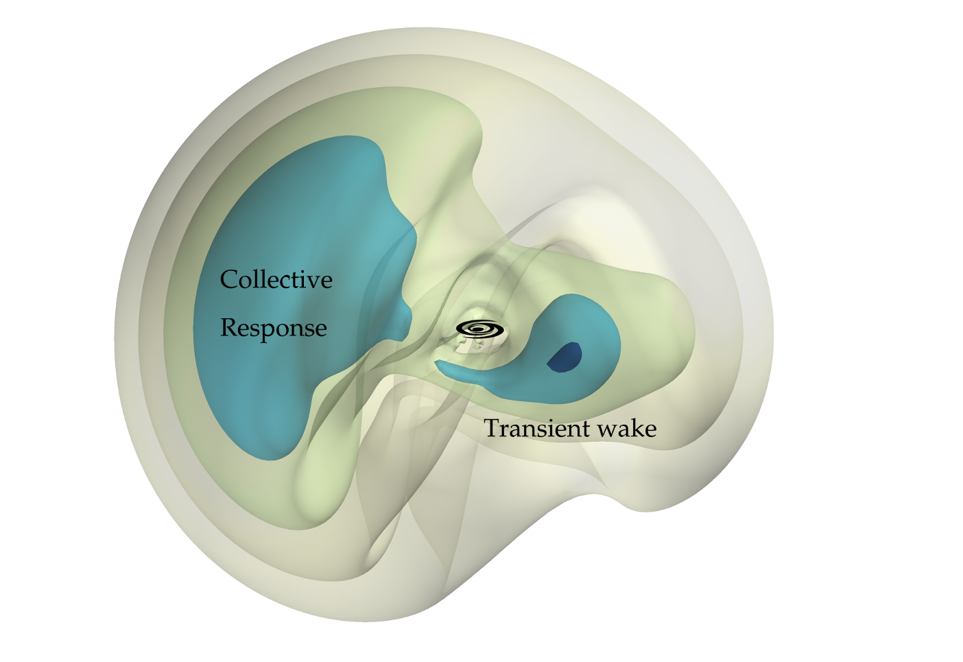
Figure 19.16: The response of the Milky-Way halo to the infall of the LMC (Adapted by Nico Garavito-Camargo from Garavito-Camargo et al. 2021).
Dynamical friction is easiest to apply to the orbits of objects with constant mass. Because accreted satellites will generally lose mass to tides (see below), they do not have constant masses during their inspiraling accretion, but supermassive black holes or globular clusters with sizes much less than their tidal radius do have constant mass. Modeling the background density as an isothermal sphere (Chapter 5.6.2), we have that \(\rho(r) = \sigma^2 / [2\pi\,G\,r^2]\), where \(v_c = \sqrt{2}\,\sigma\). Considering a massive object with mass \(M\) on a circular orbit (so \(X = 1\) in Equation 19.39), the dynamical friction deceleration is \begin{equation}\label{eq-hierarchgal-dynfric-isotherm-adf} |\vec{a}_\mathrm{DF}(\vec{x}_M,\vec{v}_M)| = 0.428\,{GM\over r^2}\,\ln \Lambda\,, \end{equation} where \(0.428 \approx \mathrm{erf}(X)-(2/\sqrt{\pi})\,X\,\exp(-X^2)\) for \(X=1\). We can then compute the time \(t_\mathrm{DF}\) for a massive object to sink to \(r=0\) starting from radius \(r_M\) by assuming that the object is at all times on a circular orbit, because the dynamical-friction deceleration then remains given by Equation (19.43) at all times, and we assume that \(\ln \Lambda\) is constant. This is most easily done by following the evolution of the angular momentum and finding when it goes to zero. The initial specific angular momentum is \(L = r\,v_c\) and the dynamical-friction acceleration is equivalent to a specific torque \(N = -r\,|\vec{a}_\mathrm{DF}(\vec{x}_M,\vec{v}_M)|\). The equation of motion is then given by Equation (3.5), which can be written as \begin{equation}\label{eq-hierarchgal-dynfric-isothermal-constant-mass-0} r\,v_c\,\mathrm{d}r = -0.428\,GM\,\ln \Lambda\,\mathrm{d}t\,. \end{equation} Integrating both sides from \(r=r_M\) to \(r=0\) between \(t=0\) and \(t_\mathrm{DF}\), we find that \begin{align} t_\mathrm{DF} & = {1.17 \over \ln \Lambda}\,{v_c\,r_M^2\over GM} = {1.65 \over \ln \Lambda}\,{\sigma\,r_M^2\over GM}= {0.186\over \ln \Lambda}\,{M_\mathrm{enc}(r_M)\over M}\,t_\mathrm{dyn}\quad (\mathrm{constant\,mass})\,,\label{eq-hierarchgal-dynfric-tdf} \end{align} where in the final step, we have written \(t_\mathrm{DF}\) in terms of the dynamical time from Equation (2.27) and the total mass \(M_\mathrm{enc}(r_M)\) enclosed within \(r_\mathrm{M}\). This is, as promised, a more rigorous version of Equation (19.42). Thus, the dynamical friction time scale for an object of mass \(M\) in galactic halos scales as \(M_\mathrm{enc}(r_M)/ M\) times the dynamical time. Massive objects with masses close to the enclosed mass at their radius are therefore expected to spiral into the center over the age of the Universe.
We can test this formula using numerical orbit integration of orbits in an isothermal (logarithmic) potential including the deceleration from Equation (19.39). For an object with \(M_\mathrm{enc}(r_M)/ M = 25\), we find evolution shown in Figure 19.17.
[29]:
from galpy.orbit import Orbit
from galpy.potential import (LogarithmicHaloPotential,
                             ChandrasekharDynamicalFrictionForce)
r_init= 5.
lnLambda= 7.
lp= LogarithmicHaloPotential(normalize=1.)
vc= lp.vcirc(r_init)
Menc= lp.mass(r_init)
M= Menc/25.
tdf= 0.186/lnLambda*Menc/M*lp.tdyn(r_init)
cdfc= ChandrasekharDynamicalFrictionForce(\
    GMs=M,const_lnLambda=lnLambda,
    sigmar=lambda r: vc/numpy.sqrt(2.),
    minr=1e-2) # avoid haywire when r~0
o= Orbit([r_init,0.,1.,0.,0.,0.])
ts= numpy.linspace(0.,1.3*tdf,1001)
o.integrate(ts,lp+cdfc,method='dop853_c')
figure(figsize=(10,4.5))
subplot(1,2,1)
o.plotr(gcf=True,color='k')[0]
axvline(tdf,color='k')
text(22.,4.3,r'$t_\mathrm{DF}$',size=18.)
subplot(1,2,2)
o.plot(d1='x',d2='y',gcf=True,color='k',
      xrange=[-r_init*1.1,r_init*1.1],
      yrange=[-r_init*1.1,r_init*1.1])
gca().set_aspect(1.);

Figure 19.17: The inspiral of a massive body due to dynamical friction.
We see that even though the object does not stay on a particularly circular orbit during its orbital decay, the \(t_\mathrm{DF}\) estimate from Equation (19.45) provides a good estimate of the decay time scale. By adjusting \(M_\mathrm{enc}(r_M)/ M\), you can check that when \(M_\mathrm{enc}(r_M)/ M\) becomes larger, the estimate gets better and better.
Dynamical friction causes the orbits of massive accreted satellite galaxies to decay towards the central galaxy, where they may merge entirely with the host, but such galaxies lose mass along the way to tidal forces. As the satellite loses mass, the magnitude of the dynamical friction deceleration decreases and it takes longer for the orbit to decay compared to the constant mass case. To assess the effect of mass loss on \(t_\mathrm{DF}\), we repeat the previous analysis in an isothermal halo, but assume that the object loses all of its mass as it spirals towards \(r=0\). A simple model that happens to be quasi-realistic, is that this mass loss is such that \(M(r) = M\,r/r_M\), where \(M\) and \(r_M\) are the initial mass and radius, respectively. Then Equation (19.44) becomes \(r\,v_c\,\mathrm{d}r = -0.428\,GM\,\left(r/r_M\right)\,\ln \Lambda\,\mathrm{d}t\), with solution \begin{align} t_\mathrm{DF} & = {0.372\over \ln \Lambda}\,{M_\mathrm{enc}(r_M)\over M}\,t_\mathrm{dyn}\quad (\mathrm{mass\,loss})\,.\label{eq-hierarchgal-dynfric-tdf-massloss} \end{align} This is exactly a factor of two longer than the dynamical friction time scale for constant mass from Equation (19.45). While the mass in reality may not be linearly proportional to \(r\), it should be \(M(r) \propto r^\gamma\) with \(0 \leq \gamma \leq 1\) as mass loss generally increases towards the center where tidal forces are larger. Then Equation (19.46) is multiplied by \(1/(2-\gamma)\) and \(t_\mathrm{DF}\) is somewhere between the values from Equations (19.45) and (19.46). Regardless of the exact mass-loss history, Equation (19.46) therefore provides an estimate of the inspiral time scale for satellite galaxies that is accurate to within a factor of two or so. We conclude that compact and extended massive objects with masses within a few orders of magnitude of the enclosed mass where they are orbiting are expected to spiral into the center over the age of the Universe.
19.4.2. Tides
Extended objects, such as globular clusters and satellite galaxies (which we will generally refer to as satellites in this section), orbiting within a galaxy are affected by tidal forces from their host. These tidal forces act in two main ways:
The steady, slowly-varying component of the tidal force limits the extent of the satellite to a tidal radius beyond which stars are irrevocably lost to the host.
The quickly-varying component provides tidal shocks to the satellite, injecting energy into it and causing stars and dark matter to escape.
These regimes are separated at the dynamical time in the outer parts of the satellite subject to tidal forces. If the tidal force varies on time scales longer than this dynamical time, the satellite is able to re-equilibrate in response to the tidal forcing and bodies within the tidal radius remain bound to the object. If the tidal force varies much more quickly than the satellite’s dynamical time, too much energy is injected too quickly and the satellite is unable to adjust internally, instead responding by expelling some constituent bodies.
The canonical example of a steady tidal force is a globular cluster on a circular orbit within a galaxy. As we will see below, we can determine a tidal radius for this situation that is such that cluster stars within the tidal radius remain within the cluster at all future times. However, the steady tidal force can vary slowly over time, for example, when a massive satellite galaxy spirals into the center on an approximately circular orbit because of dynamical friction as discussed in the previous section. In this case, the tidal radius remains a useful concept, but it slowly shrinks over time as the satellite is exposed to a stronger and stronger tidal field. The canonical example of the quickly-varying tidal force is a satellite plunging through the disk of its host galaxy on a highly eccentric orbit. During its disk passage, such a satellite feels a tidal force that strongly varies in time, shocking the system. As the satellite travels far away from its pericenter, the tidal force vanishes and the satellite remains puffed up by the interaction. Star clusters and satellite galaxies on less eccentric orbits feel a combination of the two effects. They orbit close enough to the host’s center that the tidal force is significant over most of its orbit, providing a steady component that limits the size of the system. Additionally, the tidal force peaks strongly and over a short period during each pericenter or disk passage, providing a recurring shock to the system that leads to ongoing mass loss.
In this section, we give the basic mathematical framework behind the tidal radius and tidal shocks and then we describe some consequences of these for the evolution of globular clusters and dwarf galaxies orbiting within galaxies. Because the dynamics of satellites orbiting within a host galaxy is most easily investigated in a frame orbiting with the object, we first need to derive the mathematical framework describing dynamics in rotating reference frames.
19.4.2.1. Dynamics in rotating reference frames
As we discussed in Chapter 3.1, Newton’s laws of motion only hold in an inertial (non-accelerating) reference frame. To describe the motion of particles in an accelerating reference frame, additional fictitious forces need to be included in the equations of motion. We will focus here on deriving the equations of motion in a reference frame that is rotating with a constant frequency with respect to an inertial reference frame. This is the relevant setting for describing the equations of motion in the frame of an object on a circular orbit around the center of a galaxy and it is also the appropriate setup for investigating orbits in bars or steadily-rotating spiral structure and we will use it for that purpose in Chapter 20.
We can derive the equations of motion in the rotating reference frame by relating the position, velocity, and acceleration in the rotating reference frame to the same quantities in the inertial reference frame and then substituting in Newton’s second law of motion. The position \(\vec{r}\) in the rotating reference frame is given in terms of the position \(\vec{x}\) in the inertial frame as \begin{equation}\label{eq-hierarchgal-inertial-to-rotating-frame} \vec{r} = \vec{R}(t)\,\vec{x}\,, \end{equation} where \(\vec{R}(t)\) is the time-dependent rotation matrix defining the rotating frame; we will drop the explicit time dependence going forward. The time derivative \(\dot{\vec{R}}\) of the rotation matrix is given by \(\dot{\vec{R}} = -\boldsymbol{\Omega}\times\vec{R}\). This follows from the fact that \(\vec{S} = \dot{\vec{R}}\,\vec{R}^T\) is a skew-symmetric matrix, because \(\vec{R}\,\vec{R}^T = \vec{I}\). A skew-symmetric matrix has only three independent components and we can arrange these as a vector \(\boldsymbol{\Omega} = (\Omega_x,\Omega_y,\Omega_z)\), such that \begin{equation} \vec{S} = \left(\begin{matrix} 0 & \Omega_z & -\Omega_y\\ -\Omega_z & 0 & \Omega_x\\\Omega_y & -\Omega_x & 0\end{matrix}\right)\,. \end{equation} We then have that \(\dot{\vec{R}} = \vec{S}\,\vec{R} = -\boldsymbol{\Omega}\times\vec{R}\), because multiplying a skew-symmetric matrix with a vector or matrix is equivalent to the cross product. We have defined \(\boldsymbol{\Omega}\) here as the frequency of the rotating frame as seen from the inertial frame.
To relate the velocities in the two frames, we take the time derivative of Equation (19.47) and find \begin{align} \dot{\vec{r}} & = -\left(\boldsymbol{\Omega} \times \vec{R}\right)\,\vec{x}+\vec{R}\,\dot{\vec{x}}= -\boldsymbol{\Omega}\times\vec{r}+\vec{R}\,\dot{\vec{x}}\,,\label{eq-hierarchgal-vel-rotframe} \end{align} where the second equation is derived using the equivalency of the cross product to skew-matrix multiplication as \(\left(\boldsymbol{\Omega} \times \vec{R}\right)\,\vec{x} = -\vec{S}\,\vec{R}\,\vec{x} = -\vec{S}\,\vec{r} = \boldsymbol{\Omega} \times \vec{r}\). One more time derivative relates the accelerations, which we can simplify in a similar manner to \begin{align} \ddot{\vec{r}} & = -\dot{\boldsymbol{\Omega}}\times\vec{r} -2\,\boldsymbol{\Omega}\times\dot{\vec{r}} -\boldsymbol{\Omega}\times\left(\boldsymbol{\Omega}\times\vec{r}\right) +\vec{R}\,\ddot{\vec{x}}\,.\label{eq-hierarchgal-accel-rotframe-1} \end{align}
In the inertial frame \(\ddot{\vec{x}} = \vec{g}\) using Newton’s second law, where \(\vec{g}\) is the force field. For our purposes, this is always the gravitational field \(\vec{g} = -\nabla_{\vec{x}} \Phi\). Because \(\vec{R}\,\nabla_{\vec{x}} = \nabla_{\vec{r}}\), Equation (19.50) becomes \begin{align} \ddot{\vec{r}} & = -\dot{\boldsymbol{\Omega}}\times\vec{r} -2\,\boldsymbol{\Omega}\times\dot{\vec{r}} -\boldsymbol{\Omega}\times\left(\boldsymbol{\Omega}\times\vec{r}\right) -\nabla \Phi(\vec{r})\,,\label{eq-hierarchgal-accel-rotframe} \end{align} where we have dropped the subscript in \(\nabla\), because the entire equation is now written in terms of quantities in the rotating frame, so it is clear that \(\nabla = \nabla_{\vec{r}}\). This is the final form of the equations of motion in a rotating reference frame.
Comparing Equation (19.51) to Newton’s second law in an inertial frame, we see that we can continue using Newton’s second law in a rotating reference frame if we define the entire right-hand side of Equation (19.51) to be the field. In addition to the actual physical field \(-\nabla \Phi(\vec{r})\), we have to introduce three fictitious forces (which we here give as fields, i.e., forces per unit mass):
The centrifugal field \(-\boldsymbol{\Omega}\times\left(\boldsymbol{\Omega}\times\vec{r}\right)\),
the Coriolis field \(-2\,\boldsymbol{\Omega}\times\dot{\vec{r}}\),
and the Euler field \(-\dot{\boldsymbol{\Omega}}\times\vec{r}\) for variable rotation frequencies.
Alternatively, we can derive the equations of motion from Equation (19.51) using the Lagrangian formalism from Chapter 3.3. To do this, we write down the Lagrangian in terms of rotation-frame quantities: \begin{equation}\label{eq-hierarchgal-lagrangian-rotframe} \mathcal{L} = m\,{\left|\dot{\vec{r}}+\boldsymbol{\Omega}\times\vec{r}\right|^2\over 2}-m\Phi(\vec{r})\,, \end{equation} where we have used Equation (19.49) and that \(\vec{R}\,\vec{R}^T = \vec{I}\). The generalized momentum from Equation (3.26) is then \begin{equation} \vec{p} = \frac{\partial \mathcal{L}}{\partial \dot{\vec{r}}} = m\,\dot{\vec{r}}+m\,\boldsymbol{\Omega}\times\vec{r}\,, \end{equation} The magnitude of the specific momentum is equal to that of the velocity in the inertial frame. From now on we set \(m=1\), because mass drops out of the equations of motion as usual. The Euler-Lagrange equation (3.27) then again leads to Equation (19.51). We can also compute the Hamiltonian from Equation (3.32) \begin{equation}\label{eq-hierarchgal-hamiltonian-rotframe} H = {|\vec{p}|^2\over 2}-\boldsymbol{\Omega}\left(\vec{r}\times\vec{p}\right)+\Phi(\vec{r}) = {|\vec{p}|^2\over 2}-\boldsymbol{\Omega}\,\vec{L}+\Phi(\vec{r})\,, \end{equation} using \(\vec{a}\,\left(\vec{b}\times\vec{c}\right)= \vec{c}\,\left(\vec{a}\times\vec{b}\right)\) and that \(\vec{r}\times\vec{p} = (\vec{R}\,\vec{x})\times\vec{p} = \vec{R}\,\left(\vec{x}\times\left[\vec{R}^T\,\vec{p}\right]\right) = \vec{R}\,\left(\vec{x}\times\dot{\vec{x}}\right) = \vec{R}\,\vec{L}\) and \(\boldsymbol{\Omega}\,\vec{R} = \boldsymbol{\Omega}\) to obtain the final form.
The usefulness of computing the Hamiltonian in the rotating frame is that it allows us to find an integral of the motion. When \(\boldsymbol{\Omega}\) is constant and the potential is static in the rotating frame, then the Hamiltonian in Equation (19.54) does not explicitly depend on time. Following Equation (3.38), this means that the Hamiltonian is conserved. Its value is known as the Jacobi integral \(E_J\) and it is given in terms of the energy \(E\) and angular momentum \(\vec{L}\) in the inertial frame as \begin{equation}\label{eq-hierarchgal-jacobi} E_J = E -\boldsymbol{\Omega}\,\vec{L}\,, \end{equation} because \(E = |\vec{p}|^2/2+\Phi(\vec{r})\). Thus, in a steadily-rotating, non-axisymmetric gravitational potential such as a bar, the energy and angular momentum are not separately conserved, but their combination as the Jacobi integral is conserved. We can also express the Jacobi integral in terms of \((\vec{r},\dot{\vec{r}})\) as \begin{align}\label{eq-hierarchgal-jacobi-intermsof-poteff} E_J & = {|\dot{\vec{r}}|^2\over 2} -{|\boldsymbol{\Omega}\times\vec{r}|^2\over 2} +\Phi(\vec{r})\,, \end{align} where the last two terms define the effective potential \begin{equation}\label{eq-hierarchgal-poteff} \Phi_\mathrm{eff} = \Phi -{|\boldsymbol{\Omega}\times\vec{r}|^2\over 2}\,. \end{equation} However, this effective potential only accounts for the centrifugal force, not for the Coriolis or Euler forces. In terms of the effective potential, the equation of motion from Equation (19.51) can be written as \begin{align} \ddot{\vec{r}} & = -\dot{\boldsymbol{\Omega}}\times\vec{r} -2\,\boldsymbol{\Omega}\times\dot{\vec{r}} -\nabla \Phi_\mathrm{eff}\,,\label{eq-hierarchgal-accel-rotframe-in-terms-of-poteff} \end{align} The effective potential is a useful concept, because in rotating frames with constant \(\boldsymbol{\Omega}\), the surface \(\Phi_\mathrm{eff} = E_J\) for a given star is the zero-velocity surface beyond which the star cannot venture: from Equation (19.56), it is easy to see that \(\Phi_{\mathrm{eff}} \leq E_J\). We will use this zero-velocity surface to derive the tidal radius below.
19.4.2.2. The distant-tide approximation
When considering the effect of tides on galactic satellites, it is typically the case that the size of the satellite under investigation is much smaller than the impact parameter (for an encounter with another object) or than the scale over which the perturbing tidal field changes significantly. In this case, we can approximate the tidal field using a Taylor expansion that simplifies the analysis of the effect of the tidal field. This approximation is known as the distant-tide approximation.
Working in a reference frame in which the satellite’s center of mass is at the origin, we can expand the perturbing gravitational field \(-\nabla \Phi(\vec{x},t)\) using a Taylor series at \(\vec{x} = 0\), dropping all higher-order, non-linear terms. Its components \(-\partial \Phi/\partial x_i\) are then given by \begin{equation}\label{eq-hierarchgal-ttensor} -{\partial \Phi \over \partial x_i} \approx -{\partial \Phi \over \partial x_i}\Bigg|_{\vec{x} = 0} - \sum_j{\Phi_{ij}\,x_j}\,,\; \mathrm{where}\quad \Phi_{ij}(t) = {\partial^2 \Phi(\vec{x},t) \over \partial x_i\partial x_j}\Bigg|_{\vec{x}=0} \end{equation} is the tidal tensor (sometimes defined with a negative sign). It is straightforward to demonstrate that the trace of the tidal tensor is \(4\pi G\) times the density at \(\vec{x}=0\). Considering then the motion of a body in the satellite at location \(\vec{x}\) and velocity \(\vec{v}'\), we can break up its velocity as \(\vec{v}' = \vec{v}_\mathrm{cm}'+ \vec{v}\), where \(\vec{v}_\mathrm{cm}'\) is the velocity of the center of mass. The acceleration of the center of mass due to the perturbing force is \(\dot{\vec{v}}_\mathrm{cm}' = -{\partial \Phi / \partial x_i}\big|_{\vec{x} = 0}\), and the acceleration of the body with respect to the center of mass due to the perturbation is \begin{equation}\label{eq-hierarchgal-distanttide-vdot} \dot{\vec{v}} = \dot{\vec{v}}' - \dot{\vec{v}}_\mathrm{cm}' = - \sum_j{\Phi_{ij}\,x_j}\,. \end{equation}
In the distant-tide approximation, therefore, the contribution from the perturbing field to the acceleration measured relative to that of the center of mass is fully determined by the tidal tensor. Of course, the relative acceleration also has contributions from the internal mass distribution of the satellite that need to be added to obtain the full acceleration. The effect of the tidal field is to stretch or compress an object along axes determined by the eigenvectors of the tidal tensor. The strength of the tidal field can be quantified by the eigenvalues of the tidal tensor. It is clear from Equation (19.59) that a positive eigenvalue corresponds to a compressive field, while a negative eigenvalue is a stretching field. For example, the eigenvalues of the Milky Way’s tidal field at the location of Pal 5—a globular cluster with prominent tidal tails (see below)—are estimated to be \((122,-142,122)\,\mathrm{Gyr}^{-2}\):
[30]:
from numpy.linalg import eigvals
from galpy.orbit import Orbit
from galpy.potential import (MWPotential2014,ttensor)
o= Orbit.from_name('Pal5')
# ttensor returns minus tidal tensor as defined in this book
-eigvals(ttensor(MWPotential2014,o.R(),o.z(),
                 ro=8.,vo=220.))
[30]:
Thus, the eigenvalue with the largest magnitude is negative and, therefore, Pal 5 is significantly stretched in one direction. But there are two positive eigenvalues of almost the same magnitude, indicating significant compression in the other two directions. Integrating the orbit of Pal 5 backwards in time for 3 Gyr, we can determine how the tidal field changes in time. Figure 19.18 displays the time dependence of the three eigenvalues.
[31]:
ts= numpy.linspace(0.,-3.,5001)*u.Gyr
o.integrate(ts,MWPotential2014)
lambdas= numpy.array([-eigvals(ttensor(MWPotential2014,o.R(t),o.z(t),
                                       ro=8.,vo=220.))
                     for t in ts])
figure(figsize=(6,4))
plot(ts,lambdas)
xlabel(r'$t\,(\mathrm{Gyr})$')
ylabel(r'$\lambda\,(\mathrm{Gyr}^{-2})$');

Figure 19.18: The eigenvalues of the tidal tensor along Pal 5’s past orbit.
We see that one eigenvalue is always negative and typically this is the eigenvalue with the largest magnitude. Thus, Pal 5 is significantly stretched along most parts of its orbit. There is a second eigenvalue that is always positive and only slightly smaller in magnitude than the always-negative eigenvalue. A third eigenvalue has the same value as one of the other two eigenvalues for most of the orbit (although which eigenvalue it coincides with changes over time), but it displays significant spikes at regular intervals. Correlating this behavior with the orbit of Pal 5, one finds that these spikes correspond to disk crossings, with the largest spikes occurring when the disk crossing happens very close to the center. During spikes, the eigenvalue with the largest magnitude is positive, so Pal 5 is strongly compressed during disk crossings. The compressive tidal field during disk crossings is a prime example of a tidal shock (see below). That the third eigenvalue coincides with one of the others between disk crossings is a consequence of Pal 5 mainly orbiting far from the disk where the halo is spherical: in a spherical mass distribution, two of the eigenvalues of the tidal tensor are equal.
19.4.2.3. The tidal radius
Satellites in a constant tidal field, or one that is varying only very slowly, have a limiting radius beyond which stars and dark matter are unbound due to the tidal field. This is most easily understood in the case of two point-masses orbiting each other. In the galactic context, each of these point masses represents a centrally-concentrated system such that the potential far from its center is approximately Keplerian. But the results that we obtain in this case are not so different from those of the more realistic treatment of galactic tides that we discuss below.
We consider two point masses \(M\) and \(m\) orbiting their center of mass on circular orbits. The frequency of this circular orbit is \begin{equation}\label{eq-hierarchgal-tides-rotframefreq} \Omega = \sqrt{{G(M+m)\over r^3}}\,, \end{equation} where \(r\) is the separation between the two masses. From Equation (19.57), the effective potential in the frame rotating with angular frequency \(\Omega\) is \begin{equation}\label{eq-hierarchgal-tides-phieff-pointmasses} \Phi_\mathrm{eff} = -G\,\left({M \over |\vec{r}-\vec{r}_M|}+{m\over |\vec{r}-\vec{r}_m|}+{M+m \over 2r^3}\,\left[x^2+y^2\right]\right)\,, \end{equation} where \(\vec{r}_M\) and \(\vec{r}_m\), respectively, are the position of mass \(M\) and \(m\). Setting \(GM=1\), \(Gm=1/7\), and \(\Omega = 1\), we find the effective potential in Figure 19.19.
[32]:
def phieff(x,y,Omega,GM=1.,Gm=1./7.,
          aux=False):
    sep= ((GM+Gm)/Omega**2.)**(1./3.)
    # Position relative to the center of mass
    xM= -Gm/(GM+Gm)*sep
    xm= GM/(GM+Gm)*sep
    if aux:
        return xm,xM,sep
    return -GM/numpy.sqrt((x-xM)**2.+y**2.)\
            -Gm/numpy.sqrt((x-xm)**2.+y**2.)\
            -Omega**2./2.*(x**2.+y**2.)
xs= numpy.linspace(-1.75,1.75,201)
ys= numpy.linspace(-1.75,1.75,201)
figure(figsize=(6,6))
galpy_plot.dens2d(phieff(xs[:,None],ys[None,:],1.).T,
                  origin='lower',
                  xrange=[xs[0],xs[-1]],
                  yrange=[ys[0],ys[-1]],
                  xlabel=r'$x$',
                  ylabel=r'$y$',
                  justcontours=True,gcf=True,
                  cntrcolors='k',cntrls='-',
                  levels= sorted(numpy.hstack(([-1.70769, # L1
                                                -1.91325, # L2
                                                -2.002,   # L3
                                                -1.58],   # L4/L5
                                               numpy.linspace(-1.59,-1.68,3),
                                               numpy.linspace(-1.75,-2.25,3),
                                               numpy.linspace(-2.35,-3.5,5)))))
plot([*phieff(xs[0],ys[0],1.,aux=True)[:2]],[0.,0.],marker='x',color='k',ls='none')
t= text(-1.3,0.,r'$L_1$',fontsize=18.)
t.set_bbox(dict(facecolor='w',alpha=0.85,edgecolor='none'))
t= text(1.35,0.,r'$L_2$',fontsize=18.)
t.set_bbox(dict(facecolor='w',alpha=0.85,edgecolor='none'))
t= text(0.5,0.15,r'$L_3$',fontsize=18.)
t.set_bbox(dict(facecolor='w',alpha=0.85,edgecolor='none'))
t= text(0.2,1.,r'$L_4$',fontsize=18.)
t.set_bbox(dict(facecolor='w',alpha=0.85,edgecolor='none'))
t= text(0.2,-1.05,r'$L_5$',fontsize=18.)
t.set_bbox(dict(facecolor='w',alpha=0.85,edgecolor='none'))

Figure 19.19: The effective potential of two point masses in the co-rotating frame.
We see that the effective potential near the centers of the two point masses—indicated by the crosses—is circularly symmetric and dominated by the \(\Phi \propto 1/r\) behavior of an individual point-mass potential. Far away from both point masses, contours of the effective potential surround both point masses and orbiting bodies feel the combined effect of two point masses. In the transition region, the effective potential is complex and characterized by five extrema: three saddle points along \(y=0\) and two maxima at \(y\neq 0\). These extrema are known as Lagrange points. Equation (19.58) demonstrates that objects at rest at the extrema of the effective potential, remain at rest when \(\dot{\boldsymbol{\Omega}}=0\) as we assumed here. The Lagrange points are very important in the dynamics of solar-system bodies and the Earth-Sun Lagrange points are highly important for galaxy science as well, as satellites such as Gaia and JWST orbit the \(L_2\) Lagrange point to maintain a balanced position pointing away from the Sun, Earth, and Moon.
The contour \(\Phi_3\) through the Lagrange point \(L_3\) is the most important one for investigating tidal effects. As can be seen from Figure 19.19, this contour separates the region where contours circle one of the centers from that where contours circle both centers (or L4 or L5). As we saw above, bodies are restricted to orbit in the region \(\Phi_{\mathrm{eff}} \leq E_J\). Because near the center of each body, the effective potential decreases as one approaches the center, bodies with \(E_J < \Phi_3\) inside of the \(\Phi_3\) contour are therefore restricted to orbit only one of the centers. Thus, bodies near the smaller \(m\) mass with \(E_J < \Phi_3\) remain near \(m\) at all future times, while bodies with \(E_J < \Phi_3\) near the larger \(M\) or with energies \(E_J > \Phi_3\) stray very far away from the smaller \(m\) object. Example orbits for each of these three cases are shown in Figure 19.20: the left orbit starts at \(x\) slightly larger than \(L_3\), the middle orbit stars at \(x\) slightly smaller than \(L_3\) (both have initial \(y=\dot{x}=\dot{y}=0\) and thus \(E_J < \Phi_3\)), and the right orbit has \(E_J > \Phi_3\).
[33]:
from galpy.potential import (KeplerPotential,
                             RotateAndTiltWrapperPotential,
                             NonInertialFrameForce)
from galpy.orbit import Orbit
kpM= KeplerPotential(amp=1.)
kpm= KeplerPotential(amp=1./7.)
xm,xM= phieff(0.,0.,1.,aux=True)[:2]
kpMr= RotateAndTiltWrapperPotential(pot=kpM,offset=[-xM,0.,0.])
kpmr= RotateAndTiltWrapperPotential(pot=kpm,offset=[-xm,0.,0.])
nip= NonInertialFrameForce(Omega=1.)
figure(figsize=(12,5))
for ii,(rstart,phistart) in enumerate(zip([0.6,0.57,0.587],[0.,0.,0.4])):
    o1= Orbit([rstart,0.,0.,0.,0.,phistart])
    ts= numpy.linspace(0.,10.,1001)
    o1.integrate(ts,kpMr+kpmr+nip)
    subplot(1,3,ii+1)
    o1.plot(d1='x',d2='y',gcf=True,ylabel=r'$y$' if ii ==0 else None)
    # overplot the effective potential
    galpy_plot.dens2d(phieff(xs[:,None],ys[None,:],1.).T,
                      origin='lower',
                      xrange=[xs[0],xs[-1]],
                      yrange=[ys[0],ys[-1]],
                      xlabel=r'$x$',
                      justcontours=True,
                      cntrcolors='k',cntrls='-',
                      levels= sorted(numpy.hstack(([-1.70769, # L1
                                                    -1.91325, # L2
                                                    -2.002,   # L3
                                                    -1.58],   # L4/L5
                                                   numpy.linspace(-1.59,-1.68,3),
                                                   numpy.linspace(-1.75,-2.25,3)))),
                      gcf=True)
    plot([*phieff(xs[0],ys[0],1.,aux=True)[:2]],[0.,0.],
         marker='x',color='k',ls='none')
    if ii > 0:
        gca().yaxis.set_major_formatter(NullFormatter())
tight_layout()

Figure 19.20: Orbits just inside and outside of the \(L_3\) Lagrange point in the co-rotating frame of two point masses.
As expected, we see that the left orbit remains near \(m\) at all times, the middle orbit stays near \(M\), and the right orbit orbits both at various points.
In the context of tides, the \(m\) object is the satellite that is tidally disturbed by the host \(M\) object. It is then clear that the \(\Phi_3\) contour around \(m\) defines the limiting radius of the satellite. Orbits within this contour with \(E_J < \Phi_3\) remain bound to \(m\). While the \(\Phi_3\) contour is not spherical, we can approximate it as a sphere with a radius equal to the separation between \(L_3\) and the location of \(m\). This radius is known as the tidal radius \(r_J\) (also known as the Jacobi radius, the Roche radius, or the Hill radius depending on the context). Because \(L_3\) is a saddle point, we can find its position numerically as the minimum of \(\Phi_\mathrm{eff}\) at \(y=0\) between the two objects. When we calculate this minimum by direct grid-minimization for a wide range of mass ratios and a few values of \(\Omega\) (which sets \(r\) through Equation 19.61), we find that there is an approximate power-law relation \(r_J/r \propto (m/M)^{1/3}\) that describes the numerical result well over many orders of magnitude in \(m/M\) for all \(\Omega\).
We can, in fact, derive the power-law relation analytically. To do this, we evaluate the effective potential from Equation (19.62) at \(y=0\) \begin{equation}\label{eq-hierarchgal-tides-phieff-pointmasses-y0} \Phi_{\mathrm{eff},y=0} = -G\,\left({M \over |x-x_m+r|}+{m\over |x-x_m|}+{M+m \over 2r^3}\,x^2\right)\,, \end{equation} where we used \(x_M = x_m-r\). In terms of \(r_J\), the minimum occurs at \(x=x_m-r_J\), so we equate the derivative of \(\Phi_{\mathrm{eff},y=0}\) to zero at this \(x\): \begin{equation} {\mathrm{d} \Phi_{\mathrm{eff},y=0} \over \mathrm{d} x}\Bigg|_{x=x_m-r_J} = {M \over (r-r_J)^2}-{m\over r_J^2}-{M+m \over r^3}\,(x_m-r_J)=0\,. \end{equation} If \(m/M \ll 1\), we can use a version of the distant-tide approximation to Taylor-expand the first term in powers of \(r_J/r\) and truncate the series at the linear term. Also using that \(x_m=M\,r/(M+m)\), we then find \begin{equation} {M \over r^2}\,\left(1+2\,{r_J\over r}\right)-{m\over r_J^2}-{M \over r^2}+{(M+m)\,r_J \over r^3}=0\,. \end{equation} Again assuming that \(m/M \ll 1\), we arrive at \begin{equation}\label{eq-hierarchgal-tides-rJ} r_J = \left({m\over 3M}\right)^{1/3}\,r\,. \end{equation} This is exactly the power-law behavior that we discussed above. A numerical calculation demonstrates that even though we derived this result in the distant-tide approximation, it approximately holds even when \(m\approx M\). As we will see below, interpreting \(M\) as the mass within \(r\), this equation also approximately holds for extended mass distributions and it is therefore often used as the definition of the tidal radius. A useful, alternative way to write Equation (19.66) is in terms of the mean density of the satellite \(\bar{\rho}_s \propto m/r_J^3\) and the mean density \(\bar{\rho}_h \propto M/r^3\) within the tidal and orbital radius, respectively \begin{equation}\label{eq-hierarchgal-tides-rJ-as-dens} \bar{\rho}_s = 3\,\bar{\rho}_h\,. \end{equation} Thus, tidal forces limit a satellite’s extent such that its mean density within the tidal radius approximately matches the mean density of the host within the radius at which the satellite orbits.
Stars and dark matter can escape tidally-limited satellites when internal or external perturbations (e.g., the disk shocks discussed below) cause their Jacobi integral to exceed \(\Phi_3\). Because \(L_3\) separates the region where bodies can remain within the satellite orbiting its center from the region where objects orbit the host, escaping bodies are often said to escape through the \(L_3\) Lagrange point. In the limit of small mass ratios \(m/M\), the contours through \(L_3\) and \(L_2\) coincide (see below), so stars are then said to escape through the \(L_2\) and \(L_3\) Lagrange points. However, this is actually only the case in the special situation where stars orbiting close to \(r_J\) receive a very small perturbation such that their Jacobi integral barely exceeds \(\Phi_3\). Tidal shocks, which are generally responsible for observable tidal features, produce larger perturbations that cause stars and dark matter to escape from many locations around the satellite.
To compute the tidal radius in the more realistic case of a satellite orbiting within an extended, but still spherically-symmetric host with potential \(\Phi_h(r)\), we assume that the satellite is small (in both mass and size) and that we can use the distant-tide approximation. For a low-mass satellite, we may assume that the satellite-host barycenter coincides with the center of the host. We will then assume that the satellite orbits the host on a circular orbit with frequency \(\Omega_0=\Omega(r)\) in the \(z=0\) plane. We can choose to consider the host to orbit the satellite and working in the rotating reference frame centered on the satellite then, the equations of motion of a body in the satellite are given by Equation (19.51). Here, these become \begin{align}\label{eq-merger-shearing-sheet-eom} \ddot{x} & = 2\Omega_0\,\dot{y}+\Omega_0^2\,x-{\partial \Phi \over\partial x}\,;\quad \ddot{y} = -2\,\Omega_0\,\dot{x}+\Omega_0^2\,y-{\partial \Phi \over\partial y}\,;\quad \ddot{z} = -{\partial \Phi \over\partial z}\,, \end{align} where \(\vec{r} = (x,y,z)\) is the position in the rotating frame and \(\Phi = \Phi_s + \Phi_h\) is the total satellite-plus-host potential. In the rotating reference frame, the host is located at \(\vec{r} = (-r,0,0)\) so its tidal tensor from Equation (19.59) at \(\vec{r} = (0,0,0)\) becomes \begin{align} \Phi_{h,{ij}} & = \bigg(-3\,{G\,M \over r^5}\,x_i\,x_j +{G\,M' \over r^4}\,x_i\,x_j + {G\,M\over r^3}\,\delta^{ij}\bigg)\Bigg|_{\vec{r} = (0,0,0)}= {G\,M \over r^3}\,\mathrm{diag}(-2+\gamma,1,1)\,, \end{align} where \(M=M(<r)\) is the host mass enclosed within \(r\), \(M'\) is its radial derivative, \(\gamma = \mathrm{d} \ln M / \mathrm{d}\ln r\) is its logarithmic derivative, \(\delta^{ij}\) is the Kronecker delta, and \(\mathrm{diag}(\cdot,\cdot,\cdot)\) indicates a diagonal matrix. The tidal radius again corresponds to the location \(x=-r_J\) of the \(L_3\) Lagrange point, which has \(y=\dot{y}=z=\dot{z}=\dot{x}=\ddot{x}=0\). Approximating the satellite potential in its outer regions as a point-mass potential, \({\partial \Phi_s /\partial x}|_{x=-r_J} = -{G\,M / r_J^2}\) and using that \(\Omega_0^2 = GM/r^3\) we can solve the \(x\) component of Equations (19.68) at \(x=-r_J\) to obtain \begin{equation}\label{eq-hierarchgal-tides-rJ-generalhost} r_J = \left({m\over [3-\gamma]M[< r]}\right)^{1/3}\,r\,, \end{equation} where we have again made the radial-dependence of the enclosed mass explicit. This is equation is very similar to Equation (19.66), which we derived assuming that the host is a point mass. Because \(\gamma=0\) for a point mass, they obviously agree in this case. Compared to Equation (19.66), the more general Equation (19.70) increases the tidal radius by a factor of \((1-\gamma/3)^{-1/3}\) if we set \(M = M(<r)\) in Equation (19.66). For an isothermal halo (\(\gamma = 1\)), this is only a \(\approx 15\%\) change. Because \(0 < \gamma < 3\) for realistic galactic mass profiles, the proportionality factor in the equivalent of Equation (19.67) expressing the tidal boundary as a density match between the satellite and the host is closer to one and, thus, \begin{equation}\label{eq-hierarchgal-tides-rJ-as-dens-approx} \bar{\rho}_s \approx \bar{\rho}_h\,. \end{equation}
The approximate solution from Equation (19.70) in general works very well, because the tidal radius of most satellites is far enough out in the satellite that it encloses approximately all of the mass and that the potential is close to a point-mass potential. For example, modeling a globular cluster as a Plummer sphere with mass \(M = 10^5\,M_\odot\) and a scale radius \(b=10\,\mathrm{pc}\) that is orbiting at \(10\,\mathrm{kpc}\) in a Milky-Way-like NFW halo, we find that the exact solution is \(0.1246\,\mathrm{kpc}\) while the approximate solution is \(0.1250\,\mathrm{kpc}\):
[34]:
from galpy.potential import (NFWPotential, PlummerPotential,
                             evaluater2derivs,mass)
from scipy.optimize import root_scalar
from astropy.constants import G
np= NFWPotential(mvir=1,conc=8.37,
                 H=67.1,overdens=200.,wrtcrit=True,
                 ro=8.,vo=220.)
pp= PlummerPotential(amp=1e5*u.Msun,b=10.*u.pc)
r= 10.*u.kpc
# d2phi/dr2 = GM/r^3 (gamma-2)
GMr3= G*mass(np,r)/r**3.
gamma= evaluater2derivs(np,r,0.)/GMr3+2.
exact= -root_scalar(lambda rj: ((3.-gamma)*GMr3*rj*u.kpc-pp.rforce(rj*u.kpc,0.))\
                                   .to_value(u.kpc/u.Gyr**2),
                   method="brentq",bracket=[-1,-1e-3]).root*u.kpc
approx= (mass(pp,numpy.inf)/(3.-gamma)/mass(np,r))**(1./3.)*r
print(f"""The exact solution for a Plummer sphere is {exact:.4f},
compared to the approximate solution of {approx:.4f}""")
The exact solution for a Plummer sphere is 0.1246 kpc,
compared to the approximate solution of 0.1250 kpc
They agree to better than \(1\%\).
19.4.2.4. Tidal shocks
Above we saw that when a globular cluster like Pal 5 passes through the disk, it is subjected to a strong compressive tidal field for a brief period. This shocks the cluster, injecting energy into the cluster and causing some stars to gain energies beyond the binding energy of the cluster. Thus, a disk passage leads to mass loss soon after the passage. As a cluster repeatedly passes through the disk, it loses more and more stars, which can eventually entirely dissolve the cluster. This is in fact what is expected to happen to Pal 5 during its next disk passage (Dehnen et al. 2004). This effect is known as disk shocking (Ostriker et al. 1972). A similar effect occurs when a globular cluster or satellite galaxy passes through the bulge region on a highly eccentric orbit, in which case it is known as bulge shocking.
As a cluster passes through the disk of a galaxy, the strong compressive tidal field acts along the axis perpendicular to the plane. This occurs, because relative to the center of mass, the part of the cluster that is further from the mid-plane feels a stronger force, while the part of the cluster that is closer to the mid-plane feels a weaker force; because the force changes quickly with height from the disk mid-plane, this compressive tidal force is very strong. Thus, the cluster gets compressed along the normal to the plane. We can see this explicitly for the tidal field acting on the Pal 5 cluster that we showed in Figure 19.18 above. In Figure 19.21, we display the direction of the eigenvector of the tidal tensor corresponding to the large compressive eigenvalue for a part of Pal 5’s orbit. We plot the \(x-z\) component of the vector on the left and the \(y-z\) component on the right. We see that during the peak compressional phase, the direction points along the \(z\) axis.
[35]:
from numpy.linalg import eigvalsh, eigh
from galpy.orbit import Orbit
from galpy.potential import (MWPotential2014,ttensor)
o= Orbit.from_name('Pal5')
ts= numpy.linspace(0.,-3.,5001)*u.Gyr
o.integrate(ts,MWPotential2014)
lambdas= numpy.array([-eigvalsh(ttensor(MWPotential2014,o.R(t),o.z(t),
                                       ro=8.,vo=220.))
                     for t in ts])
# Find largest compressive
eigvs= numpy.array([eigh(ttensor(MWPotential2014,o.R(t),o.z(t),
                                       ro=8.,vo=220.))[1]
                     for t in ts])
compressive_dir= numpy.array([eigv[:,ii]
                              for eigv,ii in zip(eigvs,numpy.argmax(lambdas,axis=1))])
figure(figsize=(8,5))
subplot(1,2,1)
# Plot X-Z of direction
plot(ts.to_value(u.Gyr),numpy.amax(lambdas,axis=1),
     '-',lw=0.8,zorder=-10)
skip= 100
quiver(ts.to_value(u.Gyr)[::skip],numpy.amax(lambdas,axis=1)[::skip],
       compressive_dir[::skip,0],compressive_dir[::skip,2],
      scale=10.,width=0.01)
peak_indx= numpy.amax(lambdas,axis=1) > 300.
quiver(ts.to_value(u.Gyr)[peak_indx],numpy.amax(lambdas,axis=1)[peak_indx],
       compressive_dir[peak_indx,0],compressive_dir[peak_indx,2],
      scale=10.,width=0.01)
xlim(-2.5,-1.25)
xlabel(r'$t\,(\mathrm{Gyr})$')
ylabel(r'$\lambda\,(\mathrm{Gyr}^{-2})$')
galpy_plot.text(r'$x\!-\!z$',top_left=True,size=18.)
subplot(1,2,2)
# Plot Y-Z of direction
plot(ts.to_value(u.Gyr),numpy.amax(lambdas,axis=1),
     '-',lw=0.8,zorder=-10)
quiver(ts.to_value(u.Gyr)[::skip],numpy.amax(lambdas,axis=1)[::skip],
       compressive_dir[::skip,1],compressive_dir[::skip,2],
      scale=10.,width=0.01)
peak_indx= numpy.amax(lambdas,axis=1) > 300.
quiver(ts.to_value(u.Gyr)[peak_indx],numpy.amax(lambdas,axis=1)[peak_indx],
       compressive_dir[peak_indx,1],compressive_dir[peak_indx,2],
      scale=10.,width=0.01)
xlim(-2.5,-1.25)
xlabel(r'$t\,(\mathrm{Gyr})$')
galpy_plot.text(r'$y\!-\!z$',top_left=True,size=18.)
tight_layout();

Figure 19.21: The \(x\)-\(z\) (left) and \(y\)-\(z\) (right) components of the largest compressive eigenvector of the tidal tensor along Pal 5’s past orbit.
Because the main tidal effect during a disk passage is along the \(z\) axis, to first order we can study disk shocks by only considering the energy injection in the \(z\) motion within the cluster. We will consider a cluster passing through the Milky Way disk at a typical halo velocity \(v_{z,\mathrm{cm}} \approx 100\,\mathrm{km\,s}^{-1}\). The disk thickness is \(\approx 1\,\mathrm{kpc}\), so the cluster passes through the disk in \(\tau \approx 1\,\mathrm{kpc}/(100\,\mathrm{km\,s}^{-1}) \approx 10\,\mathrm{Myr}\). The dynamical time from Equation (2.28) in the outer regions of a star cluster of mass \(m\) where the potential is approximately that of a point mass is \(t_{\mathrm{dyn}} \approx 3\pi\,r^3/[Gm])^{1/2} \approx 25\,\mathrm{Myr}\) when \(m=10^5\,M_\odot\) and \(r=30\,\mathrm{pc}\). Thus, in the outer parts of a cluster, a star moves only slightly within the cluster during the disk passage. To simplify the analysis, we can therefore use the impulse approximation and assume that the star does not move at all within the cluster during the disk passage. Because star clusters are small compared to the scale over which the galactic-disk force changes significantly, we can use the distant tide approximation and Equation (19.60) becomes \begin{equation} \dot{v}_z = - \left({\partial^2 \Phi_d\over \partial z'^2}\right)\Bigg|_{z'=z_\mathrm{cm}'}\,z\,. \end{equation} Using the impulse approximation, we obtain the total change in velocity by integrating this over the time that the cluster passes through the disk \begin{align} \Delta v_z & = -\int\mathrm{d}t\,\left({\partial^2 \Phi_d\over \partial z'^2}\right)\Bigg|_{z'=z_\mathrm{cm}'}\,z= -{2\,|g_z|\,z \over v_{z,\mathrm{cm}}'}\,,\label{eq-hierarchgal-dvz-disk-shock} \end{align} where in the second equation we assumed that the center of mass motion is linear, so \(z_\mathrm{cm}' = v_{z,\mathrm{cm}}'\,t+\mathrm{constant}\); \(|g_z|\) is the magnitude of the disk’s vertical force at the edge of the disk. Note that the change in velocity is essentially the maximum tidal force, \(|g_z|\,z/z_d\), times the duration of the shock, \(z_d/v_{z,\mathrm{cm}}'\). For a galaxy with a flat rotation curve, Equation (10.40) shows that \(|g_z| \approx 2\pi G\,\Sigma\), where \(\Sigma\) is the disk surface density (see Bovy & Tremaine 2012), such that we find that \begin{equation}\label{eq-hierarchgal-tide-diskshock-deltavz} \Delta v_z \approx -{4\pi G\Sigma\,z \over v_{z,\mathrm{cm}}'}\,. \end{equation}
To leading order the change in the mean specific vertical energy \(E_z = \sum_i v_z^2/2\) of a spherical shell at radius \(r\) in the cluster is \begin{align} \langle \Delta E_z \rangle & = {1 \over 2N}\,\sum_i{\left[2v_{z,i}\,\Delta v_{z,i} +(\Delta v_{z,i})^2\right]} \approx {8\pi^2\,G^2\,\Sigma^2 \over 3\,v_{z,\mathrm{cm}}^{'2}}\,r^2\,,\label{eq-hierarchgal-dEz-disk-shock} \end{align} where we have used that \(\langle z^2\rangle = r^2/3\) for a spherical shell in a spherically-symmetric cluster. Ignoring energy changes in the other directions (which are small), we have that \(\langle \Delta E\rangle \approx\langle \Delta E_z\rangle\). Approximating the total specific energy in the outskirts of the cluster as \(E \approx Gm/r\), the number of disk passages required to fully disrupt the spherical shell at \(r\) is then \begin{equation}\label{eq-hierarchgal-ndisrupt-diskshock} n_\mathrm{disrupt} = {|E| \over \Delta E} \approx {3Gm\,v_{z,\mathrm{cm}}^{'2} \over r^3\,8\pi^2\,G^2\,\Sigma^2}\,. \end{equation} The disruption time (Spitzer 1958; Gnedin & Ostriker 1997) is the number of required passages times the time between passages. Because a cluster passes through the disk approximately twice during each orbital period \(T_\psi\) (\(T_z = T_\psi\) in a spherical potential, because the orbital plane does not precess, and we can approximate the halo potential that the cluster mainly feels as spherical), the disruption time \(t_\mathrm{disrupt} \approx n_\mathrm{disrupt}\,T_\psi / 2\). Using that \(\Sigma \approx \sigma_d^2/[2\pi G\,z_d]\), where \(\sigma_d\) and \(z_d\) are the velocity dispersion and scale height of the disk (see Equation 10.41), we can manipulate this to \begin{equation}\label{eq-hierarchgal-tdisrupt-diskshock-approx} t_\mathrm{disrupt} \approx {\sigma^2\,v_{z,\mathrm{cm}}^{'2} \over \sigma^4_d}\,\left({z_d \over r}\right)^2\,T_\psi\,, \end{equation} where \(\sigma =\sqrt{Gm/r}\) is approximately the velocity dispersion of the cluster. The first factor is of order unity for typical values, so the disruption time is set by the ratio of the size of the cluster to the thickness of the disk. For the \(r\approx 30\,\mathrm{pc}\) outskirts of globular clusters, \(z_d / r \approx 10\), so \(t_\mathrm{disrupt}\approx 100\,T_\psi \approx 20\,\mathrm{Gyr}\). Thus, the outskirts of globular clusters are slowly, but significantly eroded by disk shocks over the lifetime of the Milky Way (and similarly in other galaxies). The Pal 5 cluster extends out to \(r\approx 100\,\mathrm{pc}\), so \(z_d / r \approx 3\) and Pal 5 has significant mass loss during each disk passage.
The derivation above ignores two important effects. The first is that stars within the cluster are not entirely held fixed in position during the shock, but instead orbit the center of mass. This tends to dampen the effect of the shock, such that the same passage leads to smaller velocity and energy changes. Stars at radii \(r\) deep inside the cluster have dynamical times \(t_\mathrm{dyn}(r) \ll \tau\), where \(\tau\) is the duration of the disk passage. For such stars, the tidal field acts adiabatically and it leaves no lasting changes to their orbits. One can parameterize the susceptibility of stars within the cluster to the tidal shock using a parameter \(x = 2\pi \tau/t_\mathrm{dyn}(r)\) (Spitzer 1987), in which case Equation (19.75) gets multiplied by an adiabatic correction \(A(x)\). Approximating orbits inside the cluster as harmonic oscillators, one finds \(A(x) = \exp(-x^2/2)\), but more realistic cluster models lead to a less steeply declining correction (Weinberg 1994). A second effect that we ignored is that higher-order energy changes can be of similar magnitude as the first-order changes that we considered here. In particular, the \(\langle (\Delta E_z)^2\rangle\) change is similar in magnitude as \(\langle \Delta E_z\rangle^2\) (Kundic & Ostriker 1995) and this causes the dispersion in energies to increase and to reach deeper in the cluster, pushing the velocity of some stars beyond the escape velocity. The \(\langle (\Delta E_z)^2\rangle\) contribution lowers the disruption time by a factor of \(\approx 2\) (Gnedin & Ostriker 1997).
Bulge shocks are similar to disk shocks, but occur when a star cluster on an eccentric orbit comes close to the galactic bulge at pericenter \(r_p\). Approximating the bulge as a point mass \(M_b\), we can estimate the velocity change as the duration of the bulge shock \(2r_p/v_\mathrm{cm}\) times the maximum tidal force \(GM_b/r_p^3\,r\) \begin{equation} \Delta v \approx {2GM_b\,r\over r_p^2\,v_\mathrm{cm}}\,, \end{equation} and the corresponding expected energy change for a shell of stars within the cluster is again the square of this. Approximating \(E \approx Gm/r\) in the outskirts of the star cluster, we find the disruption time \begin{equation} t_\mathrm{disrupt} \approx {Gm\over r}\,{r_p^2 \over G^2 M_b^2}\,{r_p^2\over r^2}\,v^2_\mathrm{cm}\,T_r = {\sigma^2\,v_{z,\mathrm{cm}}^{'2} \over \sigma^4_b}\,\left({r_p \over r}\right)^2\,T_r\,, \end{equation} where \(T_r\) is the radial period, because pericenter passages happen once every radial period (note that \(T_r = T_\psi / \sqrt{2}\) for a logarithmic halo). In the second equation, we have expressed the \(Gm/r\) and \(GM_b/r_p\) factors as \(\sigma^2\) and \(\sigma_b^2\) and we then obtain an expression that is similar to Equation (19.77) for disk shocks. However, in this case, \(v_{z,\mathrm{cm}}^{'2} \approx \sigma^2_b\), so \(t_\mathrm{disrupt}\approx (\sigma/\sigma_b\times r_p/r)^2\,T_r\) and bulge shocking is stronger than disk shocking at similar impact parameters (\(r_p/r\) and \(z_d/r\)). For a typical globular cluster that comes near the bulge, \(\sigma/\sigma_b \approx 1/30\) and \(r_p/r\approx 100\), so \(t_\mathrm{disrupt}\approx 10\,T_r\). Generally speaking, bulge shocking is thus more destructive to globular clusters than disk shocking (Aguilar et al. 1988), although for individual globular clusters which one is more important depends on its orbit.
The combination of disk and bulge shocking is highly efficient at disrupting globular clusters in the halos of galaxies. For example, in the Milky Way, more than 50% of the current globular clusters are expected to be destroyed in the next \(10\,\mathrm{Gyr}\) (Gnedin & Ostriker 1997). The efficient disruption also implies that the original populations of globular clusters were likely much larger and that galactic halos should be filled with tidal remnants from early, disrupted star clusters.
19.4.2.5. Tidal streams
We discussed tidal tails occurring in the merger of two large galaxies at the beginning of this chapter. During high-mass-ratio minor mergers, similar tidal tails form around the tidally-disrupted satellite like a star cluster or dwarf galaxy. In this case, the tails are known as tidal streams. Tidal streams form when stars from the satellite become unbound, either by attaining a Jacobi integral \(E_J > \Phi_3\) through internal two-body relaxation, or through bulge or disk shocks. Two-body relaxation causes a stellar system to evolve towards a Maxwellian velocity distribution and this velocity distribution’s high-energy tail escapes the cluster (Ambartsumian 1938; Spitzer 1940; King 1958; Henon 1969; Spitzer & Hart 1971). Two-body relaxation builds up energy changes slowly, so bodies that exceed the tidal boundary because of two-body relaxation do so at very small energy difference with the satellite itself. Disk and bulge shocks also generally produce relatively small velocity changes, e.g., for a disk shock we can write Equation (19.74) using reference values chosen to represent a globular cluster passing through the Milky-Way disk near the Sun as \begin{equation}\label{eq-hierarchgal-tide-diskshock-deltavz-refs} \Delta v_z = -0.26\,\mathrm{km\,s}^{-1}\,\left({\Sigma \over 50\,M_\odot\,\mathrm{pc}^{-2}}\right)\,\left({z\over 30\,\mathrm{pc}}\right)\,\left({100\,\mathrm{km\,s}^{-1}\over v_{z,\mathrm{cm}}'}\right)\,. \end{equation} Thus, stars and dark matter lost to tides typically have very similar positions and velocities as their parent satellite. Their subsequent orbits are then similar to that of the satellite: initially close to the satellite, they slowly drift away from it due to the small difference in orbital frequencies between the satellite and the stripped stars. As satellites keep losing more stars over time due to the continuing effect of two-body relaxation or due to multiple disk and bulge shocks, new tidally-stripped stars start drifting away from the progenitor. The structure of phase space along the orbits of star clusters and satellite galaxies with moderate eccentricities is such that the difference in orbital frequencies is confined to a single dimension (in the three-dimensional frequency space; Tremaine 1999). The result of tidal disruption is then a long, one-dimensional stream of stars emanating from the satellite. Because stars can either gain or lose orbital energy during tidal stripping—symmetrically for small satellites—two streams form: a leading stream of stars with lower orbital energies and, thus, shorter orbital frequencies, and a trailing stream of stars with higher orbital energies.
Because tidal streams extend over significant areas of the sky and result from satellite galaxies or globular clusters with not that many stars to begin with, they have very low surface brightness and are exceedingly difficult to detect. The best place to look for them is, therefore, in the Milky Way halo, where large surveys of individual stars are able to find very low surface brightness structures. A famous image—known as the field of streams (Belokurov et al. 2006)—created using SDSS data and displayed in Figure 19.22 shows off the many dwarf-galaxy and globular-cluster streams criss-crossing the Milky Way halo.
Figure 19.22: The field of streams (credit: Vasily Belokurov, Daniel Zucker, and the Sloan Digital Sky Survey; Belokurov et al. 2006).
The dominant stream in this image is the Sagittarius (Sgr) stream, a long and wide stream emanating from the Sgr dwarf galaxy (Ibata et al. 1994; Majewski et al. 2003). The Sgr stream extends from \(r\approx 20\,\mathrm{kpc}\) out to \(r \gtrsim 100\,\mathrm{kpc}\) in the distant halo and it contributes a significant number of all halo stars in the Milky Way. The field of streams also displays many smaller streams, such as the Orphan stream—with no known progenitor, but it is likely a small dwarf galaxy—and globular cluster streams. As discussed above, the Pal 5 globular cluster is in the process of tidal disruption and the field of streams prominently shows the Pal 5 stream first detected by Odenkirchen et al. (2001).
Figure 19.23 shows the Sgr and Pal 5 streams in more detail.
|
|
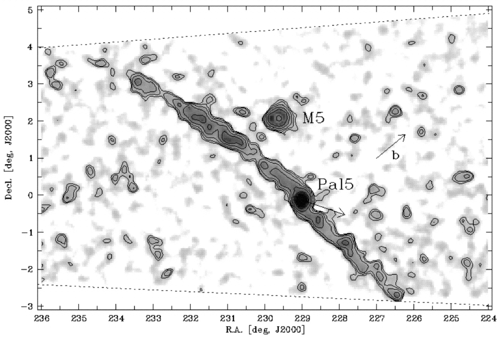
Figure 19.23: The Sgr stream traced by RR Lyrae stars (Hernitschek et al. 2017; left) and the Pal 5 stream (Odenkirchen et al. 2003; right).
The image on the left shows the spatial distribution of the Sgr stream in a Galactocentric coordinate system in which the stream lies approximately in the \(x-y\) plane. The stream is traced using variable RR Lyrae for which precise distances can be determined (e.g., Braga et al. 2015). The image on the right is a close-up view of the Pal 5 stream, with the leading tail on the left and the trailing tail on the right. The Pal 5 stream can nowadays be traced to \(\approx 15^\circ\) on either side of the progenitor (Starkman et al. 2020). As is clear from the image, the Pal 5 stream is very thin: only \(\approx 0.5^\circ\) wide, but tens of degrees long. Another famous thin stream is the GD-1 stream (Grillmair & Dionatos 2006), which in the Gaia data extends over \(\approx 100^\circ\) (Price-Whelan & Bonaca 2018). However, tidal streams are not only detected in the Milky Way. Low-surface brightness observations of external galaxies also reveal long tidal streams formed in the merger of a dwarf galaxy with its host (Martinez-Delgado et al. 2010). New observational facilities in the next decade, such as the Rubin observatory or the Roman space telescope, will even be able to detect and characterize thin globular-cluster streams in nearby external galaxies (Pearson et al. 2019).
Because the path of a tidal stream (nearly; Sanders & Binney 2013) traces out an orbit in the host potential, tidal streams quite directly measure the gravitational field and, through the Poisson equation, the mass density. Because they orbit in the galactic halo, tidal streams have become a popular method for determining the mass, radial profile, and shape of the Milky Way’s dark matter halo. Much like gravitational lensing, stream modeling does not require any assumptions of dynamical equilibrium (unlike the methods we discussed in Chapters 5, 10, and 14) and, for thin globular-cluster streams, the details of the tidal disruption process have little effect on the resulting stream. Thin streams are also sensitive probes of inhomogeneities in the galactic potential, such as the low-mass dark-matter subhalos that should be prevalent in galactic halos according to the standard cold-dark-matter paradigm. Encounters between streams and dark-matter subhalos perturb the orbits of stars in the stream, causing density and path fluctuations along the stream (Ibata et al. 2002; Johnston et al. 2002; Siegal-Gaskins & Valluri 2008; Carlberg 2009; Bovy et al. 2017). Specifically, the observed density fluctuations of the Pal 5 and GD-1 streams confirm the presence of the expected population of subhalos in the Milky Way down to \(M \approx 10^7\,M_\odot\), strongly constraining deviations from the standard cold-dark matter paradigm (Banik et al. 2021).

 .
. .
. .
.