
20.1. The (in)stability of disks
We discussed the stability of self-gravitating systems in general terms in Chapter 17.3.3 and presented various results about the stability of spherical systems. The main conclusion there was that, as long as they are not highly anisotropic, spherical self-gravitating systems are stable against any perturbation. In this section, we will demonstrate that the situation for astrophysical disks is significantly different in that typical disks are susceptible to a variety of instabilities. These instabilities manifest themselves in the form of bars, spiral structure, and warps.
Disks are unstable when the amplitude of certain perturbations grows with time rather than decays away. Self-gravity is crucial, because perturbations in non-self-gravitating systems simply phase-mix away (Chapter 17.3.2). Computing the gravitational field in axisymmetric disks—let alone perturbed, non-axisymmetric disks—is difficult and computing the self-consistent gravitational response to a disk perturbation is therefore highly non-trivial. Only a few analytical results about disk stability are therefore known and much of the research into the stability of disks has to be performed through numerical \(N\)-body simulations. Under slightly idealized circumstances, some analytical results can be derived and, luckily, these generalize well to more realistic disks. In this section, we start by deriving the main analytical disk stability criterion and then discuss the results from numerical simulations.
20.1.1. The Toomre stability criterion
The basic stability criterion for galactic disks was obtained by Toomre (1964) and it concerns the stability of razor-thin, axisymmetric disks against axisymmetric perturbations. To derive the criterion, we will calculate the density response \(\Sigma_1\) of a galactic disk with unperturbed surface density \(\Sigma_0\) to a potential perturbation \(\Phi_1\) and at the end impose the self-consistency condition that \(\Phi_1\) is sourced by \(\Sigma_1\). To compute the response, we will use the continuity equation for the density and the Jeans equations to obtain the perturbed velocities. The difficult part of this calculation is relating \(\Phi_1\) and \(\Sigma_1\), because while we could use the techniques in Chapter 7.3.2, the result would not be amenable to analytical treatment. To circumvent this issue, we make what is known as the tight-winding approximation—a form of the Wentzel (1926)-Kramers (1926)-Brillouin (1926) (WKB) approximation. Because this is the crucial approximation in the derivation that is also useful in studies of spiral structure, we start by discussing the tight-winding approximation before computing the self-consistent response of the disk.
20.1.1.1. The tight-winding approximation
Axisymmetric perturbations to razor-thin galactic disks can be written as \begin{equation}\label{eq-secevol-perturbation-density} \Sigma_1(R,t) = \Sigma_a(R,t)\,e^{if(R,t)}\,, \end{equation} where \(\Sigma_a(R,t)\) represents the slow radial variation of the amplitude and \(f(R,t)\) encodes the local shape of the perturbation. In expressions such as these here and everywhere below, it is implicitly assumed that only the real part of this complex function is physical. In the tight-winding approximation, the oscillation is rapid in the sense that \(|k\,R| \gg 1\), where \(k = \partial f / \partial R\) at a reference radius \(R_0\) where we want to compute the potential. Because the oscillation is rapid, contributions to the potential at \(R_0\) from distant regions cancel out and we can expand the surface-density perturbation from Equation (20.1) near \(R_0\) as \begin{equation}\label{eq-secevol-perturbation-density-expanded} \Sigma_1(R,t) = \Sigma_a(R,t)\,e^{ik\,(R-R_0)}\,, \end{equation} where \(k\) may depend on time and we have absorbed \(e^{if(R_0,t)}\) into \(\Sigma_a(R,t)\). The characteristic length of the perturbation is then \(2\pi/k\). Again using the tight-winding approximation, this perturbation is essentially a plane wave \(\Sigma_1(\vec{x}) \propto e^{i\,\vec{k}\cdot\vec{x}}\) with gravitational potential \(\Phi_1(\vec{x},z) \propto e^{i\,\vec{k}\cdot\vec{x}-k|z|}\). Applying this to the perturbation in Equation (20.2) and using Equation (7.9) to determine the proportionality constant, the perturbation’s gravitational potential in the mid-plane is \begin{equation}\label{eq-secevol-toomre-perturbation-pot} \Phi_1(R,t) = -{2\pi G\,\Sigma_a(R,t)\over |k|}\,e^{ik\,(R-R_0)}\,. \end{equation} Using similar reasoning, we can obtain the gravitational potential–density pair for more general tightly-wound, non-axisymmetric perturbations of the form \begin{equation}\label{eq-secevol-toomre-perturbation-pot-nonaxi} \Sigma_1(R,\phi,t) = \Sigma_a(R,t)\,e^{im\phi+if(R,t)}\,;\; \Phi_1(R,\phi,t) = -{2\pi G\,\Sigma_a(R,t)\over |k|}\,e^{im\phi+if(R,t)}\,, \end{equation} where the only additional assumption we need is that radial variations in the density are much more rapid than azimuthal ones (such that the approximate plane-wave form still holds). This result is useful when considering perturbations due to spiral structure.
20.1.1.2. The response of a cold disk
Taking a step back now, we compute the velocity and density perturbation of a cold axisymmetric galactic disk due to a potential perturbation \(\Phi_1\) without for now requiring that \(\Sigma_1\) sources \(\Phi_1\). We expand all quantities as a sum of their unperturbed values (using subscript 0) and the perturbation (using subscript 1): \begin{align}\label{eq-secevol-toomre-phi-expansion} \Phi = \Phi_0+\Phi_1\,;\quad & \Sigma = \Sigma_0+\Sigma_1\,;\\ v_{\phi} = v_{\phi,0}+v_{\phi,1}\,;\quad & v_{R} = v_{R,0}+v_{R,1}\,,\label{eq-secevol-toomre-vR-expansion} \end{align} where \(v_\phi\) is the azimuthal velocity and \(v_R\) is the radial velocity. The unperturbed values only depend on \(R\), but not on time. To compute the response, we first derive the relevant time-dependent, axisymmetric Jeans equations using similar steps as in Chapter 10.1.1. The axisymmetric, time-dependent collisionless Boltzmann equation for a razor-thin disk is (cf. Equation 10.2) \begin{align}\label{eq-collisionless-boltzmann-equil-cyl-with-time} {\partial f \over \partial t} + p_R\,\frac{\partial f}{\partial R} + \left(\frac{p_\phi^2}{R^3}-\frac{\partial \Phi}{\partial R}\right)\,\frac{\partial f}{\partial p_R}& = 0\,. \end{align} Integrating over the three components of the momentum \((p_R,p_\phi,p_z)\), we derive the continuity equation for a razor-thin disk \begin{equation}\label{eq-intevol-continuity-axi} {\partial \Sigma \over \partial t} + {1\over R}\,{\partial \over \partial R}\Big(\Sigma\,R\,v_R\Big) = 0\,. \end{equation} Multiplying Equation (20.7) by \(p_R\) and integrating over the momentum \(\vec{p}\), we similarly derive the radial Jeans equation for an axisymmetric, razor-thin disk and using the continuity equation (20.8), we can simplify this to \begin{equation}\label{eq-intevol-radialjeans-axi-with-time} {\partial v_R\over \partial t}+v_R\,{\partial v_R \over \partial R}-{v_\phi^2 \over R} = -{\partial \Phi \over \partial R}\,. \end{equation} Finally, multiplying Equation (20.7) by \(p_\phi\) and integrating over \(\vec{p}\), we derive the azimuthal Jeans equation for an axisymmetric, razor-thin disk, which we can again simplify using the continuity equation to \begin{equation}\label{eq-intevol-azimuthaljeans-axi-with-time} {\partial v_\phi\over \partial t}+v_R\,{\partial v_\phi \over \partial R} + {v_R\,v_\phi\over R}= 0\,. \end{equation}
Plugging the expansions in Equations (20.5) to (20.6) into the continuity equation (20.8) and ignoring the small, perturbed quantities, we find that \(\partial \left(\Sigma_0\,R\,v_{R,0}\right)/\partial R = 0\), which implies that \(v_{R,0} = 0\), because \(\Sigma_0\) is arbitrary. Equation (20.9) to zero-th order then implies that \(v_{\phi,0}^2 = R\,\partial \Phi / \partial R = v_c^2\). Thus, we recover the expected result that all stars in a cold, axisymmetric, unperturbed disk are on circular orbits.
Next, we work out Equations (20.9) and (20.10) while keeping terms linear in the perturbed values, which leads to \begin{equation}\label{eq-intevol-radialjeans-axi-with-time-perturbed} {\partial v_{R,1}\over \partial t} +{\partial \Phi_1 \over \partial R}-2\,{v_c\,v_{\phi,1}\over R}= 0\,;\quad {\partial v_{\phi,1}\over \partial t} -2B\,v_{R,1}= 0\,, \end{equation} where we have substitute in the Oort function \(B\) from Equation (8.33). To solve these equations, we take the Fourier transform in time, effectively looking for solutions \(\propto e^{-i\omega\,t}\) (so \(\Phi_1(R,t) = \tilde{\Phi}_1(R)\,e^{-i\omega\,t}\) and similar for the other quantities). Equations (20.11) then become \begin{align} -i\omega\,\tilde{v}_{R,1} +{\partial \tilde{\Phi}_1 \over \partial R}-2\,{v_c\,\tilde{v}_{\phi,1}\over R} & = 0\,;\quad -i\omega\,\tilde{v}_{\phi,1} -2B\,\tilde{v}_{R,1} = 0\,, \end{align} with solution \begin{align}\label{eq-intevol-toomre-vr-response-axi} \tilde{v}_{R,1} & = \phantom{-}{i\,\omega\over \kappa^2-\omega^2}\,{\partial \tilde{\Phi}_1 \over \partial R}\,;\quad \tilde{v}_{\phi,1} =-{2\,B\over \kappa^2-\omega^2}\,{\partial \tilde{\Phi}_1 \over \partial R}\,, \end{align} where we have used that \(-4B\,v_c/R = -4B\,\Omega = \kappa^2\), where \(\kappa\) is the epicycle frequency (see Equations 8.31 and 9.25). These solutions are the kinematic response of a galactic disk to an imposed axisymmetric perturbation \(\Phi_1(R,t) = \tilde{\Phi}_1(R)\,e^{-i\omega\,t}\). The density response \(\Sigma_1\) can then be computed from the perturbed continuity equation \begin{equation}\label{eq-intevol-toomre-density-response-axi} -i\omega\,\tilde{\Sigma}_1\ + {1\over R}\,{\partial \over \partial R}\Big(\Sigma_0\,R\,\tilde{v}_{R,1}\Big) = 0\,. \end{equation} We now insist that the potential perturbation \(\tilde{\Phi}_1\) is sourced by the density perturbation \(\tilde{\Sigma}_1\) and we relate them using the tight-winding approximation from Equation (20.4), which in the current notation is given by \begin{equation}\label{eq-intevol-toomre-potential-axi-tightwinding} \tilde{\Phi}_1 = -{2\pi G\,\tilde{\Sigma}_1\over |k|}\,, \end{equation} where \(\tilde{\Sigma}_1 = \tilde{\Sigma}_{1a}\,e^{if(R)}\). In Equation (20.13), \(\partial \tilde{\Phi}_1 / \partial R\) is then approximately given by \(ik\,\tilde{\Phi}_1\) near the reference point \(R_0\) and we have that \begin{align}\label{eq-intevol-toomre-vr-response-axi-tightwinding} \tilde{v}_{R,1} & = -{\omega\,k\over \kappa^2-\omega^2}\,\tilde{\Phi}_1 \,, \end{align} Similarly, in equation (20.14), the main radial variation of the argument of the radial derivative comes from \(\tilde{v}_{R,1}\) (we assume that the unperturbed density \(\Sigma_0\) varies more slowly than the perturbation), so we can replace the radial derivative by \(ik\) and simplify the resulting equation to give \begin{equation}\label{eq-intevol-toomre-continuity-sigma-vR} \tilde{\Sigma}_1\ ={k\,\Sigma_0\over \omega}\,\tilde{v}_{R,1}\,. \end{equation} Substituting in \(\tilde{v}_{R,1}\) from Equation (20.16) and then \(\tilde{\Phi}_1\) from Equation (20.15), we find that \(|k|\,\left(\kappa^2-\omega^2\right)\,\tilde{\Sigma}_1\ =2\pi G\,k^2\,\Sigma_0\,\tilde{\Sigma}_1\). For this equation to hold, we require that \begin{equation}\label{eq-intevol-dispersion-cold} \omega^2=\kappa^2-2\pi G\,\Sigma_0\,|k|\,. \end{equation} This is known as a dispersion relation as it relates the wave number \(k\) of a wave to its frequency. For the disk to be stable, only oscillating solutions should exist, which means that we require \(\omega^2 \geq 0\) for all \(k\), or \begin{equation} \kappa^2\geq 2\pi G\,\Sigma_0\,|k|\,. \end{equation} However, for large enough \(k\)—corresponding to a small-scale perturbation—this cannot hold and instead a cold stellar disk is unstable to perturbations with wave number larger than the critical wave number \(k_c\) or with wavelength smaller than the critical wavelength \(\lambda_c\) given by \begin{equation}\label{eq-intevol-toomre-critical-wavelength} k_c= {\kappa^2\over 2\pi G\,\Sigma_0}\,;\qquad \lambda_c = {2\pi\over k_c} = {4\pi^2 G\,\Sigma_0 \over \kappa^2}\,. \end{equation}
For example, in the solar neighborhood \(\Sigma_0 \approx 50\,M_\odot\,\mathrm{pc}^{-2}\) and \(\kappa \approx 40\,\mathrm{km\,s}^{-1}\,\mathrm{kpc}^{-1}\), so \(\lambda_c \approx 5.3\,\mathrm{kpc}\). Unstable perturbations grow on a characteristic time of \(\tau = 1/|\omega| = 1/\sqrt{2\pi G\,\Sigma_0\,|k|-\kappa^2}\); this time scale becomes arbitrarily short as \(|k|\) increases. Cold stellar disks are therefore violently unstable!
20.1.1.3. The response of a warm disk
Realistic galactic disks are warm rather than cold—that is, they have non-zero velocity dispersions \(\sigma\) with \(v_c/\sigma \approx 10\)—and this stabilizes the disk as the random mix of orbital phases at any location dampens the collective response to a perturbation. To compute how this happens in detail, we need to solve for the entire response of the distribution function to the perturbation and then demand that the density corresponding to the perturbed distribution function sources the perturbing potential. This can be done analytically when assuming that the razor-thin distribution function is the Schwarzschild distribution function from Chapter 10.2.2.1 and assuming that the tight-winding approximation holds. We do not derive this result here, but merely state the result: for a warm disk with radial velocity dispersion \(\sigma_R\), the radial-velocity response from Equation (20.16) is modified by a reduction factor \(\mathcal{F}(s,\chi)\) as (Kalnajs 1965; Lin & Shu 1966) \begin{align}\label{eq-intevol-toomre-vr-response-axi-tightwinding-warm} \tilde{v}_{R,1} & = -{\omega\,k\over \kappa^2-\omega^2}\,\tilde{\Phi}_1\,\mathcal{F}(s,\chi) \,, \end{align} where \(s \equiv \omega/\kappa\), \(\chi \equiv \sigma_R^2\,k^2/\kappa^2\), and \begin{equation}\label{eq-intevol-toomre-reduction} \mathcal{F}(s,\chi) = {1-s^2 \over \sin \pi s}\,\int_0^\pi \mathrm{d}\tau\,e^{-\chi\,(1+\cos \tau)}\,\sin s\tau\,\sin \tau\,. \end{equation}
In Figure 20.2, we plot the reduction factor for three different wave numbers at \(\omega = 40\,\mathrm{km\,s}^{-1}\,\mathrm{kpc}^{-1}\) as a function of velocity dispersion \(\sigma_R\) at the solar radius in the Milky Way model from McMillan (2017).
[8]:
from scipy import integrate, special
def reduction_factor_base(s,chi):
    if s == 0.: # limit s-> 0 given below this figure
        return (1.-special.ive(0,chi))/chi
    return (1.-s**2.)/numpy.sin(numpy.pi*s)\
        *integrate.quad(lambda t: numpy.exp(-chi*(1.+numpy.cos(t)))\
                            *numpy.sin(s*t)*numpy.sin(t),
                        0.,numpy.pi)[0]
def reduction_factor(kappa,sigmaR,omega,k):
    s= (omega/kappa).to_value(u.dimensionless_unscaled)
    chi= (sigmaR**2.*k**2./kappa**2.).to_value(u.dimensionless_unscaled)
    return reduction_factor_base(s,chi)
from galpy.potential import epifreq
from galpy.potential.mwpotentials import McMillan17
sRs= numpy.linspace(0.,100.,101)*u.km/u.s
figure(figsize=(6,4))
kappa= epifreq(McMillan17,8.21*u.kpc)
for k in [0.1/u.kpc,1./u.kpc,10./u.kpc]:
    plot(sRs,
         [reduction_factor(kappa,sR,40.*u.km/u.s/u.kpc,k)
          for sR in sRs],
        label=rf'$k = {k.to_value(1/u.kpc)}\,\mathrm{{kpc}}^{{-1}}$')
xlabel(r'$\sigma_R\,(\mathrm{km\,s}^{-1})$')
ylabel(r'$\mathcal{F}$')
ylim(0.,1.1)
legend(frameon=False,fontsize=17.);

Figure 20.2: The reduction factor.
We see that the response to large-scale perturbations is essentially the same as that for a cold disk, \(\mathcal{F} \approx 1\), but on smaller scales, the response is significantly suppressed and more so at smaller scales. This makes sense, as the response should be much reduced for perturbations on scales smaller than the typical epicycle amplitude, where epicyclic motions dampen the response. In Chapter 9.3.2, we saw that the typical epicycle amplitude is \(\approx \sqrt{2}\,\sigma_R / \kappa\), so significant damping occurs when \(1/k^2 \approx \sigma_R^2 / \kappa^2\) or \(\chi \approx 1\). Because cold disks are violently unstable to small-scale perturbations, this strong damping of the response helps to stabilize the disk.
Including the reduction factor, the dispersion relation from Equation (20.18) is modified for a warm disk to \begin{equation}\label{eq-intevol-dispersion-warm} \omega^2=\kappa^2-2\pi G\,\Sigma_0\,|k|\,\mathcal{F}\left({\omega\over\kappa},{\sigma_R^2\,k^2\over\kappa^2}\right)\,. \end{equation} Again, the disk is stable when \(\omega \geq 0\) for all values of \(k\).
20.1.1.4. The stability criterion
The boundary between stability and instability lies at \(\omega=0\) and, thus, satisfies \begin{equation}\label{eq-intevol-dispersion-warm-neutral-stability} \kappa^2=2\pi G\,\Sigma_0\,|k|\,\mathcal{F}\left(0,{\sigma_R^2\,k^2\over\kappa^2}\right)\,. \end{equation} The reduction factor \(\mathcal{F}(0,\chi)\) can be obtained by taking the limit of Equation (20.22) \begin{align} \mathcal{F}(0,\chi) & = {1 \over \pi}\,\int_0^\pi \mathrm{d}\tau\,e^{-\chi\,(1+\cos \tau)}\,\tau\,\sin \tau = {1-e^{-\chi}\,I_0(\chi) \over \chi}\,,\label{eq-intevol-reduction-factor-zero-omega} \end{align} where \(I_0(x)\) is a modified Bessel function of the first kind (see Chapter B.3.5, Equation B.53). Introducing a parameter \(Q_s\) defined as \begin{equation}\label{eq-intevol-toomreQs} Q_s = {\sigma_R\,\kappa \over \pi\,G\,\Sigma_0}\,, \end{equation} the stability boundary is then given by \begin{equation}\label{eq-intevol-dispersion-warm-neutral-stability-as-Qs} Q_s =4\,x^{-1}\,Q_s^{-1}\,\left[1-e^{-Q_s^2\,x^2/4}\,I_0\left({Q_s^2\,x^2\over 4}\right)\right]\,, \end{equation} where \(x \equiv |k|/k_c\) is the magnitude of the wave number relative to the critical wave number from Equation (20.20). For small values of \(Q_s\), Equation (20.27) has a solution and the disk is unstable, but for large values it does not and the disk is fully stable against axisymmetric perturbations. We can find the value of \(Q_s\) that separates these regimes numerically, by determining the value of \(Q_s\) for which the maximum of the right-hand side of Equation (20.27) is equal to \(Q_s\). To determine this maximum, we take the derivative of the right-hand side of Equation (20.27) with respect to \(x\) and set it to zero, which leads to \begin{equation} (1+2\,y)\,e^{-y}\,I_0(y)-2\,y\,e^{-y}\,I_1\left(y\right)-1=0\,, \end{equation} where \(y=Q_s^2\,x^2/4\) and we have used the first of Equations (B.55). We can numerically determine the location \(y_\mathrm{max}\) of the maximum by solving this equation and we find that the maximum occurs at \(y_\mathrm{max} \approx 0.948\).
[9]:
from scipy import special, optimize
def toomre_max_func_deriv(y):
    return ((1.+2.*y)*special.ive(0,y)
            -2.*y*numpy.exp(-y)*special.iv(1,y)-1.)
max_y= optimize.root_scalar(toomre_max_func_deriv,
                            bracket=[1e-4,100.],
                            method='brentq').root
print(f"The maximum is found at y={max_y}")
The maximum is found at y=0.9480825819349346
We can then find the stability boundary value of \(Q_s\) by evaluating the right-hand side of Equation (20.27) expressed in terms of \(y\) at the location of this maximum \(Q_s=2\,y^{-1/2}\,\left[1-e^{-y}\,I_0(y)\right] \approx 1.06897\). By convention, this numerical factor is absorbed into the definition of the stability parameter by replacing the factor of \(\pi\) in the denominator of Equation (20.26) by \(\pi \times 1.06897 \approx 3.36\). In this case the criterion for a stellar disk to be stable against axisymmetric perturbations can be written as the the Toomre stability criterion \begin{equation}\label{eq-intevol-toomre-stability-criterion} Q > 1\,,\quad \mathrm{with}\ Q = {\sigma_R\,\kappa \over 3.36\,G\,\Sigma_0}\,. \end{equation} The \(Q\) parameter is known as the Toomre \(Q\) parameter (Toomre 1964).
The most unstable wave number for a stellar disk can be found by evaluating \(x_\mathrm{max}=k_\mathrm{max}/k_c = 2\sqrt{y_\mathrm{max}}/Q_s\) at the stability boundary. This gives \(k_\mathrm{max}/k_c \approx 1.8\) or expressed in terms of the most unstable wavelength, \(\lambda_\mathrm{max}/\lambda_c \approx 0.55\). From the discussion below Equation (20.20) we can derive that in the solar neighborhood \(\lambda_\mathrm{max} \approx 3\,\mathrm{kpc}\). This implies that \(k_\mathrm{max}\,R \approx 16 \gg 1\) and the tight-winding approximation is indeed valid. As \(Q\) decreases below one, an increasing range of wavelengths on both sides of this maximally-unstable wavelength become unstable as well.
The Toomre \(Q\) parameter depends on the velocity dispersion, the epicycle frequency, and the local surface density. It makes sense that the disk is more stable when the velocity dispersion is higher and less stable when the surface density is higher. The appearance of the epicycle frequency is perhaps less intuitive, but it encodes the fact that if stars oscillate faster radially, self-gravity is less able to grow perturbations. For a given surface density, \(\kappa\) can be increased by adding, for example, a massive dark-matter halo.
In the solar neighborhood, typical values of the quantities going into Equation (20.29) are \(\sigma_R = 20\,\mathrm{km\,s}^{-1}\), \(\Sigma_0 \approx 50\,M_\odot\,\mathrm{pc}^{-2}\), and \(\kappa \approx 40\,\mathrm{km\,s}^{-1}\,\mathrm{kpc}^{-1}\), so we have that \(Q \approx 1.1\) and the solar neighborhood is marginally stable in this simplified picture (but see Figure 20.3 below).
The Toomre stability criterion is overly simplistic when applied to realistic galactic disks for at least three reasons: (i) stellar disks are not razor-thin, (ii) galactic disks typically have a significant cold gas component, which can severely affect their stability, and (iii) galactic disks are composed of gas in a variety of phases and of stellar populations with a wide range of ages, velocity dispersions, and thicknesses. All of these complications are important in establishing whether a galactic disk is stable to axisymmetric and non-axisymmetric perturbations.
20.1.1.5. The stability criterion for thick disks
When considering the effect of the finite thickness of the stellar disk, the relevant parameter is \(k h\), where \(h\) is the effective thickness of the disk. When \(k_\mathrm{max}\,h \ll 1\) for the most unstable wave number, then the effect of the finite thickness of the disk is small, because the disk effectively appears to be razor-thin to the unstable mode. Typically, \(k\,h < 1\), but not \(k\,h \ll 1\). For example, in the solar neighborhood, the effective disk thickness is \(h = \Sigma_0/(2\,\rho_0)\), with \(\rho_0 \approx 0.1\,M_\odot\,\mathrm{pc}^{-2}\) the local mid-plane density (see Equation 10.52; Holmberg & Flynn 2000). Thus, \(h \approx 250\,\mathrm{pc}\) and because the most unstable wavelength is \(\lambda_\mathrm{max} \approx 3\,\mathrm{kpc}\), we have that \(k\,h\approx 0.5\). Toomre (1964) estimated the effect of a stellar disk’s finite thickness in the limit \(k\,h \ll 1\) by approximating the disk as a uniform-density slab between \(z=-h\) and \(z=+h\), finding that the finite thickness of the disk effectively reduced the surface density \(\Sigma_0\) that enters in Equation (20.29) as \begin{equation}\label{eq-intevol-toomre-thickess-reduce-toomre} \Sigma_0 \rightarrow \Sigma_0\,\left({1-e^{-k\,h}\over k\,h}\right)\,. \end{equation} For small \(kh\), we have that this is \(\approx \Sigma_0\,(1-kh/2)\).
Vandervoort (1970) improved upon this analysis by modeling the vertical extent of the disk as a more realistic \(\mathrm{sech}^2(z/h)\) profile and by performing a formal stability analysis of this scenario, concluding that the surface density is reduced as \begin{equation}\label{eq-intevol-toomre-thickess-reduce-vandervoort} \Sigma_0 \rightarrow \Sigma_0\,\left({1\over 1+k\,h}\right)\,. \end{equation} For the solar neighborhood with \(k\,h \approx 0.5\), Equations (20.30) and (20.31) reduce \(\Sigma_0\) by \(\approx 0.8\) and \(0.65\) respectively. Because \(Q \propto \Sigma_0^{-1}\), these reductions increase \(Q\) by \(\approx 30\%\) to \(50\%\), thus significantly increasing the stability of the disk compared to the razor-thin criterion.
20.1.1.6. The stability criterion for gas disks
However, a not insignificant fraction of the mass of galactic disks is in the form of a cold gas component and this component is highly susceptible to instabilities (Safronov 1960). We can derive a similar dispersion relation and stability criterion for gaseous (“fluid”) disks using a similar procedure as we followed to derive the collisionless results above. The full derivation is left as an exercise, but we give the important ingredients of the derivation here and present the results. We assume that the gas can be described as an ideal fluid and such a fluid follows the Euler equation (17.28), which is the fluid equivalent of the Jeans equations that we relied on for stars. Again assuming a razor-thin disk—a very good approximation for the very thin gas layer in galaxies—we can write Equation (17.28) in polar coordinates as \begin{align}\label{eq-intevol-toomre-euler-radial} \frac{\partial u_R}{\partial t} +u_R\,{\partial u_R \over \partial R} -{u_\phi^2 \over R} & = - {\partial \Phi \over \partial R}-{1\over \Sigma}{\partial P \over \partial R} \,;\quad \frac{\partial u_\phi}{\partial t} +u_R\,{\partial u_\phi \over \partial R} +{u_\phi\,u_R \over R} = 0\,, \end{align} because \begin{align}\label{eq-intevol-toomre-euler-gradient} (\vec{u}\cdot \nabla)\,\vec{u} = & \left(u_R\,{\partial u_R \over \partial R} +{u_\phi\over R}\,{\partial u_R \over \partial \phi}-{u_\phi^2\over R}\right)\,\vec{\hat{e}}_R +\left(u_R\,{\partial u_\phi \over \partial R} +{u_\phi\over R}\,{\partial u_\phi \over \partial \phi}+{u_\phi\,u_R \over R}\right)\vec{\hat{e}}_\phi\,, \end{align} and we have assumed axisymmetry. The continuity equation (20.8) remains the same, but now applies to the fluid velocity \((u_R,u_\phi)\). Note that Equations (20.32) are the same as Equations (20.9) and (20.10) for stellar disks with the addition of a pressure term in the radial equation. Thus, as in our discussion of the evolution of small baryonic overdensities in the Universe in Chapter 17.1.3, the equations describing the evolution of fluids are the same as those describing collisionless systems if we add a pressure term.
To relate the pressure to the density, we assume a simple equation of state \begin{equation} P = {c_s^2\,\Sigma_0\over \gamma}\,\left({\Sigma\over \Sigma_0}\right)^\gamma\,, \end{equation} where \(c_s = \mathrm{d}P /\mathrm{d}\Sigma\) evaluated at \(\Sigma=\Sigma_0\) is the sound speed for the unperturbed density \(\Sigma_0\). Replacing the pressure by the specific enthalpy \(h = c_s^2\,(\Sigma/\Sigma_0)^{\gamma-1}/(\gamma-1)\), the right-hand side of Equation (20.32) simplifies to \(-\partial (\Phi+h)/\partial R\).
We can then again expand all quantities in terms of their unperturbed values plus a perturbation as in Equations (20.5) and (20.6) (but now also expanding the enthalpy similarly) and this leads to the same relations as in Equations (20.11), but with \(\Phi_1\) replaced by \(\Phi_1+h_1\). We then again look for solutions \(\propto e^{-i\omega\,t}\) and this leads to the same relations as in Equations (20.13), but now with \(\tilde{\Phi}_1\) replaced by \(\tilde{\Phi}_1+\tilde{h}_1\). Using the tight-winding approximation, we find the radial-velocity response \(\tilde{u}_{R,1} = -\omega\,k\,\left(\tilde{\Phi}_1+\tilde{h}_1\right)/\left(\kappa^2-\omega^2\right)\). Then we can eliminate \(\tilde{h}_1\) in favor of \(c_s\) by linearizing the equation of state, which gives \(\tilde{h}_1 = c_s^2\,\tilde{\Sigma}_1/\Sigma_0\). Using the continuity equation (20.17) in the tight-winding approximation, we can eliminate \(\tilde{h}_1\) and derive \begin{align}\label{eq-intevol-toomre-vr-response-axi-tightwinding-fluid-no-enthalpy} \tilde{u}_{R,1} & = -{\omega\,k\over \kappa^2-\omega^2+c_s^2\,k^2}\,\tilde{\Phi}_1\,, \end{align} and with the tight-winding relation between the surface density and the potential from Equation (20.15), we can then derive the dispersion relation for fluid disks \begin{equation}\label{eq-intevol-dispersion-cold-fluid} \omega^2=\kappa^2-2\pi G\,\Sigma_0\,|k|+c_s^2\,k^2\,. \end{equation} Comparing this to the dispersion relation from Equation (20.18) for a cold stellar disk, we see that the only difference is the term involving the sound speed. In particular, a pressureless fluid disk is equivalent to a cold stellar disk.
A fluid disk is stable against all axisymmetric perturbations when \(\omega^2>0\) in Equation (20.36) for all \(k\). When this condition is satisfied is easier to establish than in the stellar case, because Equation (20.36) is a quadratic function of \(k\). The stability boundary is \(0=\kappa^2-2\pi G\,\Sigma_0\,|k|+c_s^2\,k^2\). This has no solutions if the discriminant \((2\pi G\,\Sigma_0)^2-4c_s^2\,\kappa^2\) is negative and we thus arrive at the stability criterion for fluid disks (Hunter 1972) \begin{equation}\label{eq-intevol-toomre-stability-criterion-fluids} Q_g > 1\,,\quad \mathrm{with}\ Q_g = {c_s\,\kappa \over \pi\,G\,\Sigma_0}\,. \end{equation} Comparing this to the stability criterion for razor-thin stellar disks from Equation (20.37), we see that they are the same if we replace \(\sigma_R\) with the sound speed and \(3.36\) by \(\pi\). The stability criterion for fluid disks applies to any astrophysical gas disk and \(Q_g\) is an important parameter in the study of, e.g., protoplanetary disks and accretion disks around black holes. The most unstable wave number of a fluid disk is \(k_\mathrm{max} = \pi G\,\Sigma_0/c_s^2 = \kappa^2/(\pi G\,\Sigma_0) = 2k_c\) with \(k_c\) from Equation (20.20), where we have used that \(Q_g=1\) at the stability boundary. Therefore, \(\lambda_\mathrm{max} = 0.5\,\lambda_c\), compared to \(\lambda_\mathrm{max} \approx 0.55\,\lambda_c\) for a stellar disk. Stellar and fluid disks, therefore, have very similar unstable wavelengths. Because the sound speed of the gas is typically much lower than the velocity dispersion of the stars, gas disks are more susceptible to instabilities.
20.1.1.7. The stability criterion for multi-component disks
The final complication is that galactic disks consist of several disk components of gas in different phases and of many stellar populations with a wide range of velocity dispersions. While the discussion above demonstrates that the gas and stellar disks in the solar neighborhood appear to be separately stable, the gravitational interplay between them can cause the combined system to be unstable. Thus, we need to determine the stability of a system composed of multiple fluid and stellar disks with different properties. To derive a stability criterion for a multi-component disk, we can re-use much of the derivations above, as the Jeans, Euler, and continuity equations continue to hold for each component separately; the only ingredient that connects all of the components is the gravitational potential. Thus, the radial-velocity response \(\tilde{v}_{R,1}^i\) of stellar population \(i\) is given by Equation (20.21) for velocity dispersion \(\sigma_R^i\) and the radial-velocity response \(\tilde{u}_{R,1}^j\) of fluid component \(j\) is given by Equation (20.35) for sound speed \(c_{s,j}\). Using the continuity equation in the tight-winding approximation, we can express each radial-velocity response in terms of the perturbed surface density with Equation (20.17) and similar for the gas. The potential perturbation in the tight-winding approximation is given in terms of the perturbed surface densities as \begin{equation}\label{eq-intevol-toomre-potential-axi-tightwinding-multicomponents} \tilde{\Phi}_1 = -{2\pi G\over |k|}\,\left(\sum_i{\tilde{\Sigma}^i_1}+\sum_j{\tilde{\Sigma}^j_1}\right)\,, \end{equation} where the sum over \(i\) is over the stellar components and the \(j\) sum is over gas components. Expressing each component’s \(\tilde{\Sigma}^{i,j}_1\) in terms of its radial-velocity response, writing the radial-velocity response in terms of \(\tilde{\Phi}_1\), and canceling \(\tilde{\Phi}_1\), we arrive at the multi-component dispersion relation \begin{equation}\label{eq-intevol-dispersion-cold-multicomp} {2\pi G\,|k|}\,\left[{1\over \kappa^2-\omega^2}\,\sum_i{\Sigma^i_0\,\mathcal{F}(s,\chi^i)} +\sum_j{{\Sigma^j_0\over \kappa^2-\omega^2+c_{j,s}^2\,k^2}}\right]=1 \end{equation} for a disk composed of stellar components with surface densities and velocity dispersions \((\Sigma^i_0,\sigma_R^i)\) and gas components with surface densities and sound speeds \((\Sigma^j_0,c_{j,s})\). The stability boundary is again at \(\omega^2=0\) and can be found through the following argument. The left-hand side of Equation (20.39) increases monotonically from \(0\) at \(\omega^2 = -\infty\) to \(\infty\) at \(\omega^2 = \kappa^2\). Thus, if Equation (20.39) has no solutions with \(\omega^2 < 0\), the left-hand side evaluated at \(\omega^2 = 0\) has to be less than one (the right-hand side). Therefore, the stability criterion for a multi-component disk is given by \begin{equation}\label{eq-intevol-stability-cold-multicomp} {2\pi G\,|k|}\,\left[{1\over \kappa^2}\,\sum_i{\Sigma^i_0\,\mathcal{F}(0,\chi^i)} +\sum_j{{\Sigma^j_0\over \kappa^2+c_{j,s}^2\,k^2}}\right] < 1\,\quad \forall k\,, \end{equation} where the \(\mathcal{F}(0,\chi^i)\) reduction factor can be evaluated using Equation (20.25). This criterion was first derived by Rafikov (2001) with the important special case of a two-fluid disk—a good approximation of a galactic disk, modeling the stars as another fluid—found earlier by Jog & Solomon (1984). Unfortunately, in the general multi-component case there is no way to derive an effective ‘\(Q\)’ parameter as in Equations (20.29) and (20.37). Instead, one simply has to numerically check Equation (20.40) for all possible wave numbers (but see Elmegreen 1995 for an effective \(Q\) parameter for the two-fluid case).
We can use the multi-component stability criterion to investigate the stability of the Milky Way’s disk near the Sun in a more realistic manner. For simplicity, we model the local disk as consisting of a single gas disk and a single stellar disk with surface densities \(\Sigma_g = 10\,M_\odot\,\mathrm{pc}^{-2}\) and \(\Sigma_* = 40\,M_\odot\,\mathrm{pc}^{-2}\), respectively, \(c_s \approx 7\,\mathrm{km\,s}^{-1}\) (Holmberg & Flynn 2000), and otherwise using the same stellar velocity dispersion and epicycle frequency as above. We then show the right-hand side of Equation (20.40) in Figure 20.3.
[10]:
from astropy.constants import G
kappa= 40.*u.km/u.s/u.kpc
sigmaR= 20.*u.km/u.s
cs= 7.*u.km/u.s
Sigma_gas= 10.*u.Msun/u.pc**2.
Sigma_star= 40.*u.Msun/u.pc**2.
Sigma_total= Sigma_gas+Sigma_star
k_crit= kappa**2./(2.*numpy.pi*G*Sigma_total)
ks= numpy.linspace(1e-4*k_crit,6*k_crit,101)
def toomre_stability_two_components(k):
    return 2.*numpy.pi*G*k*(1./kappa**2.*Sigma_star
                            *reduction_factor(kappa,sigmaR,0.001*u.km/u.s/u.kpc,k)
                           +Sigma_gas/(kappa**2.+cs**2.*k**2.))
figure(figsize=(6,4))
plot(ks.to(1./u.kpc),
     [toomre_stability_two_components(k).to(u.dimensionless_unscaled) for k in ks])
axhline(1.,color='k')
axvline(2.*k_crit.to_value(1./u.kpc),color='#2ca02c')
text(2.5,0.1,r'$2\,k_c$',fontsize=18.,color='#2ca02c')
xlabel(r'$k\,(\mathrm{kpc}^{-1})$')
ylabel(r'$\mathrm{Stability\ criterion}$')
ylim(0.,1.4)
text(-0.1,1.05,r'$\mathrm{unstable}$',fontsize=18.,color='k')
text(-0.1,0.875,r'$\mathrm{stable}$',fontsize=18.,color='k');

Figure 20.3: The stability of the Galactic disk near the Sun in a two-component gas/stars model.
We see that for these parameters, the Galactic disk near the Sun is marginally unstable, with a most unstable wave number \(\approx 2\,k_c\), the expected value for a gas disk. Thus, we see that the cold gas layer has a significant de-stabilizing effect on the Galactic disk. You can change the parameters going into the stability criterion to investigate how sensitive this conclusion is to the input parameters. For example, simply increasing the stellar velocity dispersion to \(\sigma_R = 25\,\mathrm{km\,s}^{-1}\) is sufficient to stabilize the disk. Accounting for the thickness of the stellar disk using Equation (20.31) similarly suffices for stabilizing the disk. Rafikov (2001) performed a multi-component stability analysis of the solar neighborhood using Equation (20.40) for a more realistic and complex model of the local stars and gas and found that the solar neighborhood is stable, but not by a great margin.
20.1.2. The global stability of disks
The stability criterion from Equation (20.29) only directly applies to the local, axisymmetric stability of disks and \(Q > 1\) does not guarantee either global axisymmetric stability or general stability against non-axisymmetric perturbations. These types of stability are much harder to study analytically and most of what is known about disk stability comes from either \(N\)-body simulations or highly-simplified analytical treatments. We will rely on both of these in this section to obtain an understanding of the global stability of disks.
20.1.2.1. The search for a stability criterion using \(N\)-body simulations
While \(Q>1\) does not guarantee global stability against axisymmetric perturbations, \(N\)-body simulations demonstrate that disks are in fact stable against realistic axisymmetric perturbations when \(Q > 1\). This is nicely illustrated by Hohl (1971)’s \(N\)-body simulation of the axisymmetric evolution of a uniformly-rotating, razor-thin disk with a \(\Sigma(R) \propto \sqrt{1-R^2/R_d^2}\) surface-density profile out to \(R=R_d\) with a radial velocity dispersion such that \(Q=1\). The evolution of this disk over the first eight rotation periods is displayed in Figure 20.4.
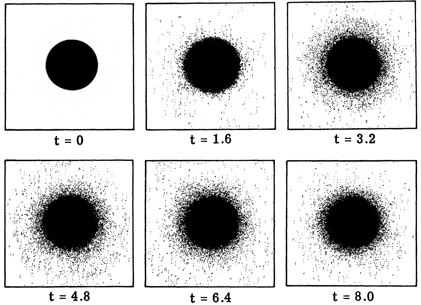
Figure 20.4: Axisymmetric evolution of a disk with initial \(Q=1\) (Hohl 1971).
The initial condition is not entirely in equilibrium and the disk pulsates slightly during the first few rotations, settling into a stable equilibrium state. However, when the axisymmetric constraint is then dropped, the disk quickly becomes violently unstable, as demonstrated in Figure 20.5.
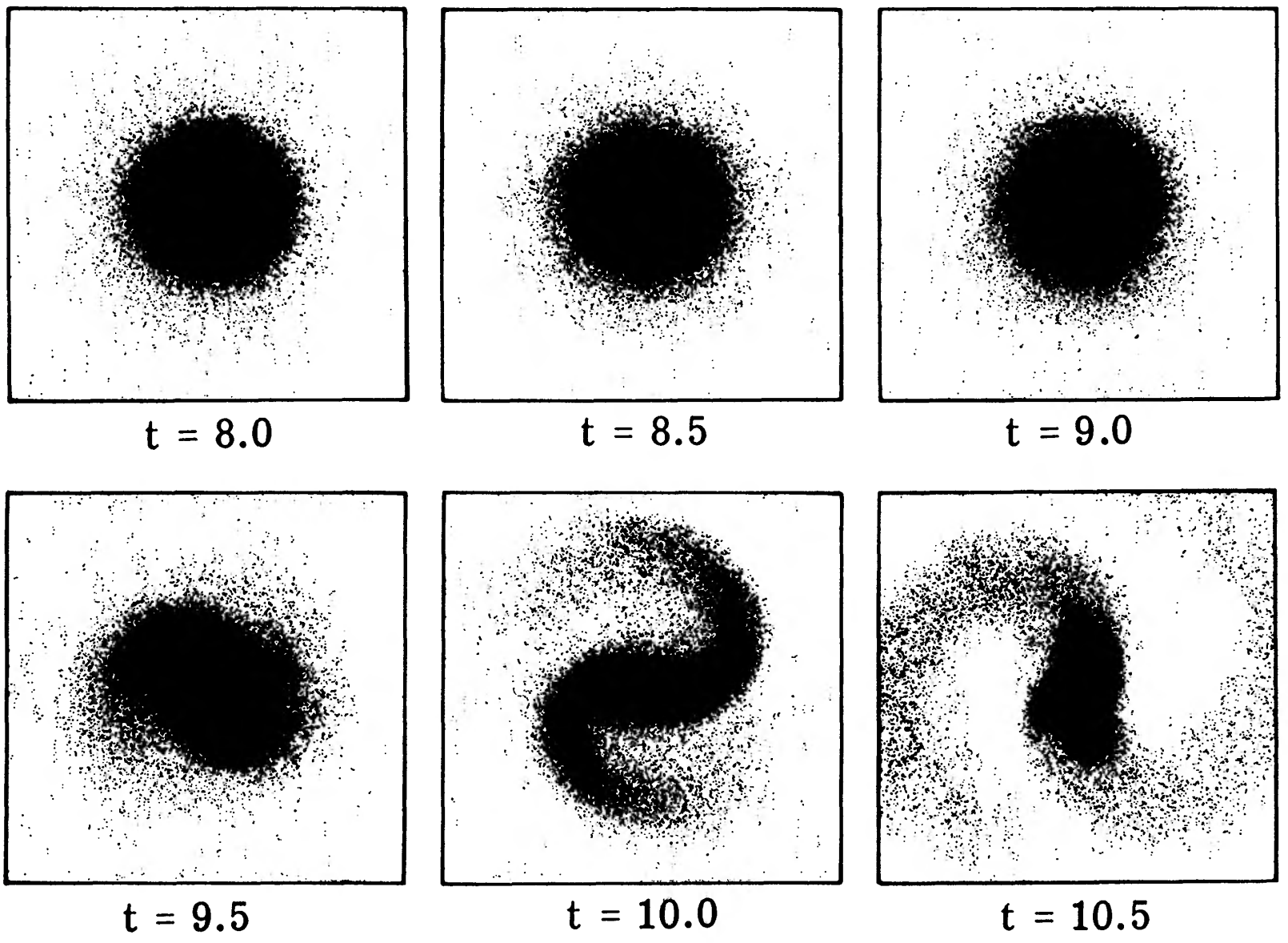
Figure 20.5: Non-axisymmetric evolution of a disk with initial \(Q=1\) (Hohl 1971).
We see that after a mere two revolutions, the axisymmetric disk undergoes a violent instability that entirely deforms the disk and leaves it with a dominant central bar sprouting strong spiral arms at its ends. While this superficially resembles some of the clearest examples of barred galaxies (e.g., NGC 1300 in Figure 1.3), this bar and its spiral arms are far stronger than those observed in external galaxies. Allowing non-axisymmetric evolution starting from the original initial condition, rather than the initial condition that had evolved to a stable state, results in an even more violent instability. Hohl (1971)’s simulations are a clear manifestation of what is known as the bar instability in disk galaxies: disk galaxies with \(Q \gtrsim 1\) are often highly unstable to the formation of a much-too-strong bar. Other early simulations of disks with \(Q > 1\) found them to be similarly unstable after only a few dynamical times (e.g., Miller et al. 1970).
Ostriker & Peebles (1973) performed a more systematic suite of \(N\)-body simulations to attempt to understand the underlying instability and devise a novel stability criterion. They focused in particular on the ratio \(T/|W|\) of the component \(T\) of the kinetic energy coming from ordered rotation (Equation 14.19) to the magnitude of the scalar potential energy \(W\) (Equation 14.21). From the conservation of the total energy and the scalar virial theorem (assuming approximate equilibrium) of Equation (14.18), the maximum value of this ratio is \(1/2\) and it occurs when the velocity dispersion is zero; any non-zero velocity dispersion causes the ratio to be \(< 1/2\). Remarkably, a wide range of simulations all pointed to a value of \(T/|W|\lesssim 0.14\) required for disk stability. That is, disks with initial \(T/|W| > 0.14\) developed instabilities that drove up the velocity dispersion until \(T/|W| \approx 0.14\), while disks with initial \(T/|W|\approx 0.14\) were found to be stable. This stability boundary of \(T/|W|\approx 0.14\) is exactly the same as that for which the sequence of Maclaurin spheroids—uniformly-rotating oblate fluid spheroids originally introduced as a model for the Earth—is secularly stable (Chandrasekhar 1969; Bardeen 1971; Ostriker & Bodenheimer 1973). Thus, Ostriker & Peebles (1973) posited that disks behave similarly to Maclaurin spheroids and that \(T/|W|\lesssim 0.14\) is a universal disk stability criterion. Exactly how the instabilities of self-gravitating, collisionless disks were similar to those of fluid spheroids remained unclear, especially because the secular instabilities of Maclaurin spheroids occur because of dissipative fluid forces and Maclaurin spheroids are only purely-gravitationally-unstable for \(T/|W|\gtrsim 0.27\) (Chandrasekhar 1969).
The Ostriker & Peebles (1973) work was highly influential in large part because they identified the presence of a massive dark halo in the visible region of disk galaxies as the most plausible way to force \(T/|W|\lesssim 0.14\) and stabilize disks against violent bar instabilities—a massive, non-rotating halo reduces \(T/|W|\) because it increases the depth of the potential well \(|W|\) without adding to \(T\). Their simulations required halos with masses one to three times as massive as the disk within the disk region to stabilize the disk. The Ostriker & Peebles (1973) work provided a strong theoretical argument in favor of dark halos that, together with the increasing evidence at the time that rotation curves of disk galaxies are flat beyond their optical radii (requiring \(M(< r) \propto r\) halos out to large radii; see Chapter 8.2.2), was instrumental in the acceptance of the dark matter paradigm (Sanders 2014). However, while we still believe in the presence of large amounts of dark matter in the visible regions of galaxies, as we will discuss below, we now know that a massive halo is no longer the only way to stabilize disks and the \(T/|W| > 0.14\) stability criterion appears to be a coincidence rather than a true stability criterion.
Our best understanding of how instabilities grow and dampen was laid out most clearly by Toomre (1981) in a highly influential conference proceedings paper. Toomre (1981) demonstrated that the way in which perturbations propagate in galactic disks, and how they grow and decay as they do so, is crucial to understanding the stability of disks. Rather than depending on a criterion based on the fraction of random energy in the system, such as \(Q\) or \(T/|W|\), Toomre (1981) identified the ratio of the scale of perturbations to the critical wavelength from Equation (20.20) as the crucial parameter determining whether instabilities grow. In addition to this, the disk must be able to sustain a growing instability and only when both criteria are satisfied does unchecked growth of instabilities such as in the simulations of Hohl (1971) occur. As we will see, these two requirements explain when disks are stable against all perturbations, why the early simulations discussed above were violently unstable, and why disk galaxies are able to sustain bars and spiral structure without being entirely consumed by instabilities.
The crucial physical mechanism for the growth of instabilities in Toomre (1981)’s picture is swing amplification (Goldreich & Lynden-Bell 1965; Julian & Toomre 1966). This is the process wherein a shearing perturbation that starts out as a leading spiral arm—with the spiral pointing in the direction of galactic rotation, rather than trailing as in almost all observed spiral galaxies (see Section 20.3 below)—undergoes strong amplification as it unwinds and turns into a trailing spiral arm. At the moment when the pattern is most open, the shear in the galactic disk and the epicyclic motions of stars are of similar magnitude and point in the same direction (against galactic rotation), keeping stars in a perturbation close together for a long enough period that self-gravity can act to quickly increase the size of the perturbation. Thus, as a leading perturbation naturally unwinds due to the shear of the disk, its amplitude grows exponentially as it swings from a leading perturbation to a trailing perturbation.
The effect of swing amplification is illustrated in Figure 20.6.
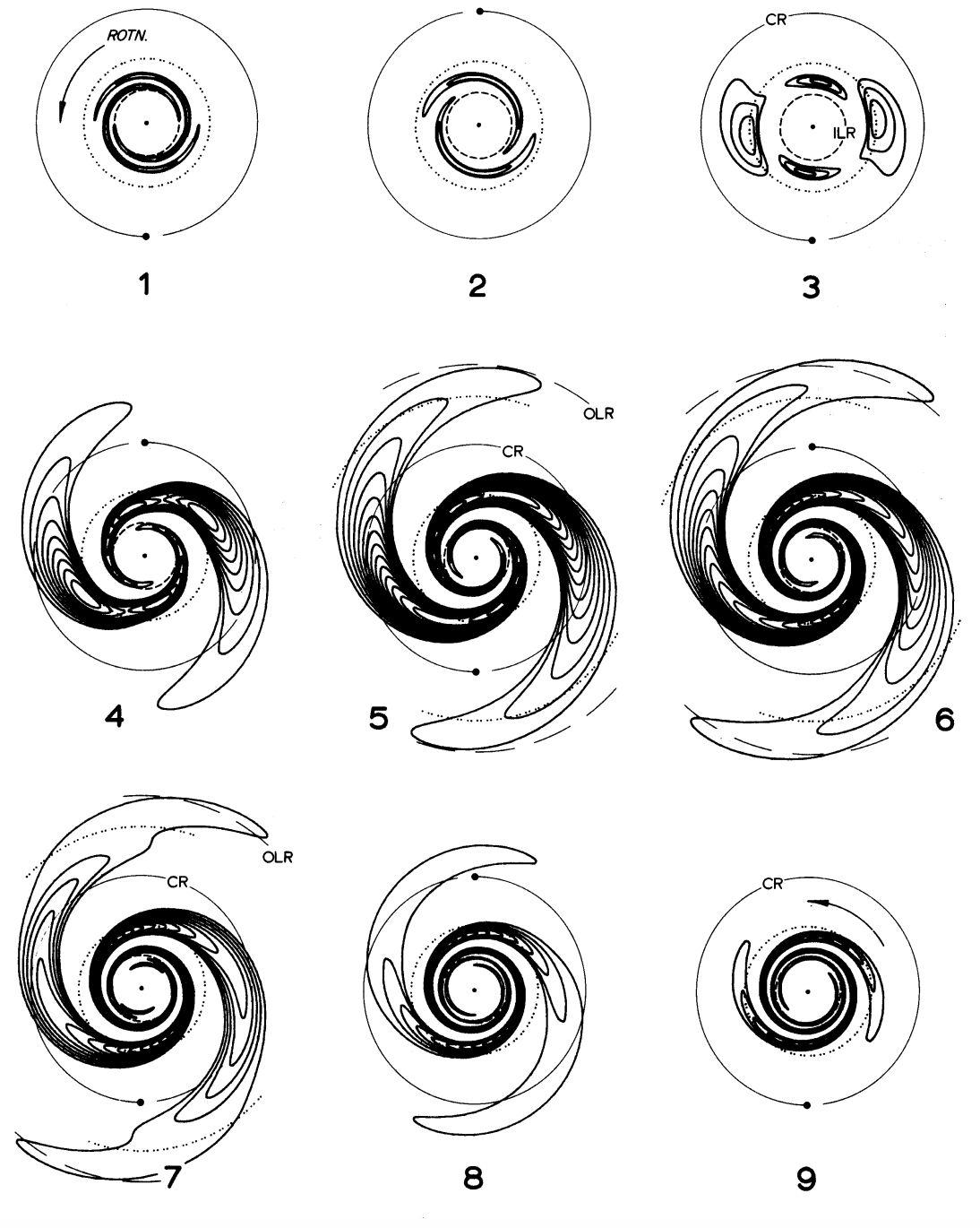
Figure 20.6: Evolution of a leading spiral perturbation through swing amplification (Toomre 1981; © Cambridge University Press 1981; reproduced with permission of Cambridge University Press through PLSclear).
This figure shows the evolution of the density of a packet of leading waves—a spatially-localized perturbation that moves across the galactic disk—as it unwinds, swing amplifies, and eventually decays, calculated using linear perturbation theory similar to that of Section 20.1.1 above. The period between each successive frame is half of the rotation period of the disk at the location where the perturbation has the same angular velocity as the disk—the corotation radius (see below)—and, thus, the pattern hardly seems to rotate although in between frames it does. As the perturbation swings from a leading to a trailing wave, its amplitude increases dramatically, before decaying slowly. At later times, the perturbation entirely disappears.
20.1.2.2. Wave mechanics of galactic disks
To understand the process of swing amplification more quantitatively, we need to study the wave mechanics of perturbations in galactic disks. Because we are considering non-axisymmetric perturbations, the starting point is a calculation of the response of a stellar or fluid disk to a non-axisymmetric perturbation and the resulting dispersion relation for self-consistent evolution. This calculation is similar to that in Section 20.1.1 and we leave the full derivation as an exercise: the starting point is the non-axisymmetric generalization of the collisionless Boltzmann equation (20.7) for stellar disks and of the Euler equation (20.32) for fluid disks. We then proceed in the same manner as before, looking for solutions of the form \(\Phi_1(R,t) = \tilde{\Phi}_1(R)\,e^{-i\omega\,t+im\,\phi}\) and similar for the other relevant quantities. The final result is that the response and the dispersion relation have the same form as derived in Section 20.1.1 if we replace \(\omega \rightarrow \omega-m\Omega\), where \(\Omega=\Omega(R)\) is the disk’s angular velocity at radius \(R\). Thus, for example, for a stellar disk, the radial velocity response becomes \begin{align}\label{eq-intevol-toomre-vr-response-axi-tightwinding-nonaxi} \tilde{v}_{R,1} & = -{(\omega-m\Omega)\,k\over \kappa^2-(\omega-m\Omega)^2}\,\tilde{\Phi}_1 \,. \end{align} Unlike in the axisymmetric case, this response can become formally infinite for oscillating perturbations (\(\omega^2 > 0\)) when the denominator vanishes; this happens at the inner Lindblad resonance (ILR) and the outer Lindblad resonance (OLR) at \begin{equation}\label{eq-intevol-lindblad} \kappa = \pm (\omega-m\Omega) = \pm m\,(\Omega_p - \Omega)\,, \end{equation} where in the second equality we have written the perturbation’s frequency in terms of the pattern speed of a pattern with \(m\)-fold symmetry: \(\omega = m\,\Omega_p\). Depending on the rotation curve, there can be multiple inner and outer Lindblad resonances. The corotation radius \(R_{\mathrm{CR}}\) (or simply “corotation”) is the radius at which \begin{equation}\label{eq-intevol-rcorot} \Omega(R_{\mathrm{CR}}) = {v_c(R_{\mathrm{CR}}) \over R_{\mathrm{CR}}} = \Omega_p \end{equation} (Equation 20.42 with \(m=\infty\)). The radii of the inner Lindblad resonances are interior to corotation where \(\Omega(R) > \Omega_p\) and, thus, corresponds to the negative sign in Equation (20.42); the outer Lindblad resonances correspond to the positive sign. We will have much more to say about the Lindblad resonances when we discuss bars and spiral structure below, because as the formally-infinite response in Equation (20.41) demonstrates, the Lindblad resonances are where the effect of perturbations are greatest. The divergence in Equation (20.41) is of course unphysical and a consequence of our assumption that the response is small such that we can use linear-perturbation theory (see Equation 20.5 to 20.6). The formally-infinite response merely indicates that the response is large.
The dispersion relation for non-axisymmetric perturbations becomes \begin{equation}\label{eq-intevol-dispersion-warm-nonaxi} (\omega-m\Omega)^2=\kappa^2-2\pi G\,\Sigma_0\,|k|\,\mathcal{F}\left({\omega-m\Omega\over\kappa},{\sigma_R^2\,k^2\over\kappa^2}\right)\,, \end{equation} for a stellar disk and \begin{equation}\label{eq-intevol-dispersion-cold-fluid-nonaxi} (\omega-m\Omega)^2=\kappa^2-2\pi G\,\Sigma_0\,|k|+c_s^2\,k^2\,, \end{equation} for a fluid disk. These equations can be solved for the frequency \(\omega(k,R)\) of a perturbation of a given wave vector \(k\) at radius \(R\) in the disk and this tells us how wave packets propagate across a galactic disk. Wave mechanics tells us that wave packets travel at the group velocity \(v_g(R) = \partial \omega / \partial k\) and the sign of this tells us whether the wave travels inwards or outwards (Toomre 1969). Let’s consider a pure stellar disk. To compute \(\omega(k,R)\) and \(v_g(R)\), it is convenient to write the dispersion relation of Equation (20.44) in the following dimensionless form \begin{equation}\label{eq-intevol-dispersion-warm-dimensionless} s^2 = 1 -|x|\,\mathcal{F}\left(s,{Q_s^2\,x^2\over4}\right)\,, \end{equation} where \(s = \left(\omega-m\Omega\right)/\kappa\), \(x = k/k_c\), and \(Q_s = 1.06897\,Q \approx (3.36/\pi)\,Q\) (see Equation 20.26 and 20.29). In terms of \(s\), corotation occurs at \(s=0\) and the inner/outer Lindblad resonances at \(s=\pm1\). We can then solve for the frequency in its dimensionless form \(s\) as a function of the dimensionless wave vector \(x\) for different values of \(Q\). Because the dispersion relation only depends on \(|s|\) and \(|x|\), we can solve for \(|s|\) as a function of \(|x|\) and obtain the solution for all possible sign combinations by mirroring this solution. This solution is shown in the left panel of Figure 20.7.
For a given value of \(\omega\), the value of \(|s|\) maps to the radius \(R\) at which a wave with frequency \(\omega\) can exist. Because \(|s| = 0\) corresponds to corotation and \(|s| = 1\) to the Lindblad resonances, we immediately see that waves can only exist between corotation and the Lindblad resonances regardless of the value of \(Q\). For disks at the edge of stability \(Q=1\), waves can exist everwhere between corotation and the Lindblad resonances, but for \(Q>1\), waves cannot exist between corotation and a \(Q\)-dependent radius that moves further away from corotation the larger \(Q\) is; this region is known as the forbidden region. As \(Q\) becomes large, waves can only exist near the Lindblad resonances. The group velocity \(v_g(R)\) can be written as \(v_g(R) = (\kappa/k_c)\,\mathrm{d} s / \mathrm{d} x\) and so is proportional to the slope of the dispersion relation as shown in the left panel of Figure 20.7. Thus, starting at \(k\approx 0\), waves propagate away from the Lindblad resonance until they get to the edge of the forbidden region, at which point they reflect off of the forbidden region and propagate towards the starting Lindblad resonance again. This is illustrated further in the right panel of Figure 20.7, where we unfold the dispersion relation into its four sign regions and we use a flat-rotation curve model to map \(s\) to \(R/R_\mathrm{CR} = 1+\sqrt{2}\,s/m\), assuming \(m=2\). We then obtain the dispersion relation for waves near the two Lindblad resonances using \(Q=1.2\) as an example.
[14]:
from scipy import integrate, optimize, special
def reduction_factor_base(s,chi):
    if s == 0.: # limit s-> 0 given below this figure
        return (1.-special.ive(0,chi))/chi
    return (1.-s**2.)/numpy.sin(numpy.pi*s)\
        *integrate.quad(lambda t: numpy.exp(-chi*(1.+numpy.cos(t)))\
                            *numpy.sin(s*t)*numpy.sin(t),
                        0.,numpy.pi)[0]
def Qs_from_Q(Q):
    return Q*1.06897 # More correct than 3.36/pi
def dispersion_relation_base(x,Q):
    Qs= Qs_from_Q(Q)
    return optimize.root_scalar(
        lambda s: s**2.-1.+x*reduction_factor_base(s,Qs**2.*x**2./4.),
        bracket=[1e-6,1.2],
        method='brentq'
    ).root
xs= numpy.linspace(0.,5.,301)
QQ= [1.,1.2,1.5,2.,4.][::-1]
figure(figsize=(12,4.5))
subplot(1,2,1)
for Q in QQ:
    ss= numpy.array([dispersion_relation_base(x,Q) for x in xs])
    plot(xs,ss,label=rf"$Q = {Q}$")
xlabel(r'$|x| = |k|/k_c$')
ylabel(r'$|s| = |\omega-m\Omega|/\kappa$')
legend(frameon=False,fontsize=17.)
subplot(1,2,2)
def R_from_s(s,m=2.,Rcr=1.):
    return Rcr*(s*numpy.sqrt(2.)/m+1.)
Q= 1.2
xs= numpy.linspace(-5.,5.,601)
line_out= plot(xs,
     [R_from_s(dispersion_relation_base(numpy.fabs(x),Q)) for x in xs])
axhline(R_from_s(1.),color=line_out[0].get_color(),ls='--')
line_in= plot(xs,
     [R_from_s(-dispersion_relation_base(numpy.fabs(x),Q)) for x in xs])
axhline(R_from_s(-1.),color=line_in[0].get_color(),ls='--')
# Path annotation, symmetrical
for ii in range(2):
    if ii == 0:
        sgn= 1.
        relevant_line= line_in
        offset= 0.
    else:
        sgn= -1.
        relevant_line= line_out
        offset= R_from_s(1.)+R_from_s(-1.)
    annotate("",xy=(-3.5,offset+sgn*0.5),xytext=(-4.5,offset+sgn*0.42),
             arrowprops=dict(arrowstyle="->",color=relevant_line[0].get_color()))
    annotate("",xy=(-1.75,offset+sgn*0.735),xytext=(-2.75,offset+sgn*0.6),
             arrowprops=dict(arrowstyle="->",color=relevant_line[0].get_color()))
    annotate("",xy=(-0.4,offset+sgn*0.55),xytext=(-1.1,offset+sgn*0.75),
             arrowprops=dict(arrowstyle="->",color=relevant_line[0].get_color()))
    annotate("",xy=(0.02,offset+sgn*0.4),xytext=(-0.3,offset+sgn*0.525),
             arrowprops=dict(arrowstyle="-",color=relevant_line[0].get_color()))
    annotate("",xy=(0.35,offset+sgn*0.545),xytext=(-0.02,offset+sgn*0.4),
             arrowprops=dict(arrowstyle="->",color=relevant_line[0].get_color()))
    annotate("",xy=(1.1,offset+sgn*0.75),xytext=(0.4,offset+sgn*0.55),
             arrowprops=dict(arrowstyle="->",color=relevant_line[0].get_color()))
    annotate("",xy=(2.75,offset+sgn*0.6),xytext=(1.75,offset+sgn*0.735),
             arrowprops=dict(arrowstyle="->",color=relevant_line[0].get_color()))
    annotate("",xy=(4.5,offset+sgn*0.42),xytext=(3.5,offset+sgn*0.5),
             arrowprops=dict(arrowstyle="->",color=relevant_line[0].get_color()))
# ILR/OLR
text(-4.75,0.175,r'$\mathrm{ILR}$',color=line_in[0].get_color())
text(-4.75,1.75,r'$\mathrm{OLR}$',color=line_out[0].get_color())
xlabel(r'$k/k_c$')
ylabel(r'$R/R_\mathrm{CR}$')
ylim(0.,1.9)
tight_layout();

Figure 20.7: Dispersion relation for stellar disks (left) and how it affects wave propagation near the inner (ILR) and outer (OLR) Lindblad resonances.
We have indicated the direction of the group velocity to demonstrate how waves propagate. Considering an initially-tightly-wound leading perturbation with \(k/k_c \ll -1\) near the ILR, the wave propagates away from the ILR along what is known as the short-wave branch. It reflects off of the boundary of the forbidden region and moves towards the ILR along the long-wave branch. It proceeds all the way to the ILR, where it reflects again onto the positive \(k\) long-wave branch, moving away from the ILR. A final reflection off of the boundary of the forbidden region sends its on its final leg along the positive \(k\) short-wave branch towards the ILR, which it approaches slowly as an ever-more-tightly-wound trailing perturbation. Near the ILR, the wave is absorbed as the wave energy is converted into random motions (Lynden-Bell & Kalnajs 1972; Mark 1974).
20.1.2.3. Swing amplification
There is, however, a major problem with the picture of wave mechanics sketched above: to derive the dispersion relation, we used the tight-winding approximation \(|kR| \gg 1\), which is satisfied along the short-wave branches, but not along the long-wave branches where \(k\) becomes arbitrarily small. As such, the picture above cannot determine what happens as the perturbation turns from a leading to a trailing perturbation and it is exactly here that swing amplification occurs. On the long branch, waves are also actually able to propagate into the forbidden region, as is obvious from Figure 20.6 above.
Understanding wave propagation without invoking the tight-winding approximation is a complicated undertaking. It is analytically tractable in a local approximation of the disk, the shearing sheet, that only considers the evolution of a small region of the disk under a perturbation while taking into account differential rotation. This was first done by Goldreich & Lynden-Bell (1965) for fluid disks and by Julian & Toomre (1966) for stellar disks. A modern, more accessible treatment of the Julian & Toomre (1966) derivation was presented by Binney (2020). Here, we present a less rigorous derivation presented by Toomre (1981) that contains all of the important physical ingredients and allows a semi-quantitative estimate of the effect of swing amplification to be made.
In the shearing sheet, we consider a rotating patch of the disk that is small enough that we can linearize the equations of motion in a local, approximately-Cartesian coordinate system. For a patch centered on \((R,\phi) = (R_0,\Omega_0\,t)\), where \(\Omega_0 = \Omega(R_0)\), the two coordinates of the shearing sheet are \begin{align}\label{eq-intevol-shearing-sheet} x & = R-R_0\,;\quad y = R_0\,(\phi-\Omega_0\,t)\,. \end{align} To derive the equations of motion in this rotating reference frame, we need to include the fictitious centrifugal and Coriolis field (see Chapter 19.4.2.1). We have, in fact, already done close to this in Equations (19.68) in the context of tides. Here, we are only interested in the \((x,y)\) part of the motion (assumed to be contained within the \(z=0\) plane) and the difference is that the patch is centered on \(R_0\) rather than on the origin; Equations (19.68) then become \begin{align}\label{eq-intevol-shearing-sheet-eom} \ddot{x} & = R_0\,\Omega_0^2+2\,\Omega_0\,\dot{y}+\Omega_0^2\,x-{\partial \Phi \over\partial x}\,;\quad \ddot{y} = -2\,\Omega_0\,\dot{x}-{\partial \Phi \over\partial y}\,. \end{align}
We then write the gravitational potential \(\Phi\) as the sum \(\Phi = \Phi_0 + \Phi_1\) of the unperturbed, axisymmetric potential \(\Phi_0(x)\) and the perturbation \(\Phi_1(x,y,t)\). The axisymmetric gravitational field is \begin{align} -{\mathrm{d} \Phi_0 \over \mathrm{d} x} & = -{\mathrm{d} \Phi_0 \over \mathrm{d} R} = -R\,\Omega^2 \approx -R_0\,\Omega_0^2 - 2\,R_0\,\Omega_0\,\Omega_0'\,x - x\,\Omega_0^2\,, \end{align} where we used that \(\Omega \approx \Omega_0 + \Omega_0' x\) with \(\Omega_0' = \mathrm{d} \Omega / \mathrm{d} R\) at \(R_0\). With this, Equations (20.48) can then be written as \begin{align}\label{eq-intevol-shearing-sheet-eom-waxi} \ddot{x} -2\,\Omega_0\,\dot{y}& = 4\,\Omega_0\,A_0\,x -{\partial \Phi_1 \over\partial x}\,;\quad \ddot{y} +2\,\Omega_0\,\dot{x} = -{\partial \Phi_1 \over\partial y}\,, \end{align} where \(A_0 = A(R_0)\) is the Oort constant from Equation (8.34). In the absence of a perturbing potential \(\Phi_1\), the \(y\) equation of motion for a star with angular momentum \(L_z = R_0\,\Omega_0^2\) can be integrated to \(\dot{y} = -2\,\Omega_0\,x\), because \(\dot{y} = 0\) at \(x=0\) for a star with this angular momentum. The \(x\) equation of motion then becomes \(\ddot{x} = 4\,\left(\Omega_0\,A_0-\Omega_0^2\right)\,x= -\kappa^2\,x\), where \(\kappa_0 = \kappa(R_0)\) is the epicycle frequency (see Equations 8.34 and 9.14). Thus, the full solution is \begin{align} x & = X\,\cos\left(\kappa\, t + \alpha\right)\,;\quad y = -2\,{\Omega_0\over \kappa_0}\,X\,\sin\left(\kappa\, t + \alpha\right) + y_0\,, \end{align} where \(X\), \(\alpha\), and \(y_0\) are integration constants. This is exactly the usual epicycle solution for a star with guiding-center radius \(R_0\) (Equation 9.23). Thus, the shearing sheet contains the essential dynamics of the differentially-rotating disk: shear and epicyclic motions with frequency \(\kappa\). As we already discussed after Equation (9.23), the epicyclic motion is in the direction opposite to galactic rotation, as is the shear. For realistic disk mass distributions, the epicycle frequency \(\kappa\) and the shear \(2A\) are also of similar magnitude. This coincidence in direction and magnitude is crucial to the mechanism of swing amplification: it means that as a perturbation transitions from a leading to a trailing shape, stars’ epicyclic motions keep them within the perturbation longer than they do at other times. This kinematic lingering allows self gravity to quickly increase the amplitude of the perturbation.
We now consider a perturbing wave \(\Phi_1 \propto e^{i\vec{k}\cdot\vec{x}}\) in the shearing sheet. This wave is oriented with an angle \(\gamma\) with respect to the \(x\) axis with positive angles towards negative \(y\), such that the angle is negative for a leading spiral and positive for a trailing arm. Julian & Toomre (1966) demonstrated that the wave evolves in a way that keeps \(\vec{k}\cdot\vec{x}\) constant for stars on circular orbits in the unperturbed potential. Along such a circular orbit, \(\dot{y} = -2A_0\,x\) from Equation (20.50), so constancy of \(\vec{k}\cdot\vec{x}\) requires that \(k_x(t) = k_x(t_0) +2A_0\,k_y\,(t-t_0)\) or \(\dot{k}_x = 2A_0\,k_y\). Written in terms of the time dependence of the angle \(\gamma\), this is \begin{equation}\label{eq-intevol-shearing-sheet-dtangammadt} {\mathrm{d}\tan \gamma \over \mathrm{d} t} = 2\,A_0\,. \end{equation} Thus, the perturbation shears just as the disk does and the perturbation acts as a material arm. Because of the one-to-one mapping of time and \(\gamma\), we will use \(\tan \gamma\) as the time coordinate below.
We then consider the evolution of the perpendicular displacement \(\xi\) from the perturbation, which is \begin{equation}\label{eq-intevol-shearing-sheet-xi} \xi = x\,\sin \gamma + y\,\cos \gamma\,. \end{equation} The equation of motion of \(\xi\) follows from Equations (20.50) with the field due to \(\Phi_1\) obtained by solving the Poisson equation in the shearing sheet. Following the same derivation as in the discussion of the tight-winding approximation in Section 20.1.1.1 above (but note that we do not need to invoke the tight-winding approximation itself), we have that \(\Phi_1(\vec{x}) = -2\pi G\,\Sigma_1/|k|\) and assuming that the perturbed surface density \(\Sigma_1\) results from displacements of the unperturbed density \(\Sigma_0\), we have that \(\Sigma_1 \approx \Sigma_0\,|k|\,\xi\). To account for the effect of random motions, we ad hoc multiply this by the same reduction factor \(\mathcal{F}(s,\chi)\) from Equation (20.22) that applied in the axisymmetric stability analysis from Section 20.1.1 above (we will specify how to set \(s\) and \(\chi\) below). The gravitational perturbing field is then \begin{equation}\label{eq-intevol-shearing-sheet-perturb-field} \vec{g}_1 = 2\pi G\,\Sigma_0\,\xi\,\vec{k}\,\mathcal{F}(s,\chi)\,. \end{equation}
Combining Equations (20.53), (20.54), and (20.52) with the equations of motion of \(x\) and \(y\), we can derive the following equation \begin{equation}\label{eq-intevol-shearing-sheet-xi-eom-1} \ddot{\xi} + \tilde{\kappa}(\gamma)\,\xi = 2\pi G\,\Sigma_0\,\xi\,|k|\,\mathcal{F}(s,\chi)\,, \end{equation} where \begin{equation} \tilde{\kappa}(\gamma) = \kappa_0^2 -8\,\Omega_0\,A_0\,\cos^2\gamma+12 A_0^2\,\cos^4\gamma\,. \end{equation} This is the equation of a spring with external forcing, with a spring constant \(\tilde{\kappa}(\gamma)\) that depends on time. When the perturbation is a tightly-wound leading or trailing arm, \(\cos \gamma \ll 1\) and \(\tilde{\kappa} \approx \kappa_0\). Displacements are then simply the normal epicycle oscillations. But when the perturbation is close to open with \(\cos \gamma \approx 1\), the spring constant is much reduced. For example, for a flat rotation curve, \(2A_0 = \Omega_0\) and \(\kappa^2 = 2\,\Omega_0^2\), so \begin{equation} \tilde{\kappa}(\gamma) = \kappa_0^2\,\left(1 -2\,\cos^2\gamma+{3\over 2}\,\cos^4\gamma\right)\quad (v_c = \mathrm{constant})\,. \end{equation} In the absence of self-gravity, Equation (20.55) is \(\ddot{\xi} + \tilde{\kappa}(\gamma)\,\xi = g_1(t)\), where \(g_1(t)\) is an external forcing and the spring constant \(\tilde{\kappa}(\gamma)\) determines the dynamics. In the flat rotation curve example, it depends on time as given in Figure 20.8.
Because of self-gravity, the forcing due to the perturbation is itself proportional to \(\xi\) (Equation 20.54), we can bring it to the left-hand side of Equation (20.55) and we end up with another spring-like equation \begin{equation}\label{eq-intevol-shearing-sheet-xi-eom-2} \ddot{\xi} + S(\gamma)\,\xi =0\,, \end{equation} where we can now express the effective spring rate \(S(\gamma)\) as \begin{equation} S(\gamma) = \kappa_0^2 -8\,\Omega_0\,A_0\,\cos^2\gamma+12 A_0^2\,\cos^4\gamma- {\kappa_0^2\over X}\,\sec\gamma\,\mathcal{F}\left(s,{Q_s^2\over 4\,X^2\,\cos^2\gamma}\right)\,, \end{equation} where we have defined \begin{equation}\label{eq-intevol-shearing-sheet-X} X = {\lambda_y \over \lambda_c} = {\kappa_0^2\over 2\pi G\,\Sigma_0\,k_y}\,, \end{equation} using the critical wavelength \(\lambda_c\) from Equation (20.20) and where again \(Q_s = 1.06897\,Q \approx (3.36/\pi)\,Q\). Because the patch is centered on the corotation radius, it makes sense to set \(s=0\) in this equation (but note that the results here and below do not depend strongly on the exact value of \(s\)). The effect of self gravity is to lower the spring rate even further than we saw above, such that it can even become negative, indicating exponential growth of the displacements. For example, for a disk with a flat rotation curve with \(Q = 1.5\) and \(X=2\) we compare \(S(\gamma)\) to \(\tilde{\kappa}^2\) from above in Figure 20.8.
[15]:
X, Q= 2., 1.5
Qs= Qs_from_Q(Q)
gammas= numpy.linspace(-numpy.pi/2.,numpy.pi/2.,101)
figure(figsize=(5,3))
plot(gammas*180./numpy.pi,
     1.-2.*numpy.cos(gammas)**2.+3./2.*numpy.cos(gammas)**4.,
    label=r'$\tilde{\kappa}^2 / \kappa_0^2$')
plot(gammas*180./numpy.pi,
     1.-2.*numpy.cos(gammas)**2.+3./2.*numpy.cos(gammas)**4.
    -(1./X/numpy.cos(gammas)
      *numpy.array([reduction_factor_base(0,Qs**2./4./X**2./numpy.cos(gamma)**2.)
                   for gamma in gammas])),
    label=r'$S / \kappa_0^2$')
xlabel(r'$\gamma\,(\mathrm{degree})$')
ylim(-0.3,1.1)
legend(frameon=False,fontsize=17.);

Figure 20.8: The effective spring constant in a stellar disk with (\(S / \kappa_0^2\)) and without (\(\tilde{\kappa}^2 / \kappa_0^2\)) the effects of self gravity and random motions.
We see that the effective spring constant does indeed become negative over a wide range of \(\gamma\). Changing \(Q\) and \(X\) in the code above, you can see that \(X\) is the most important parameter in determining whether the spring constant becomes negative for some range of angles, with \(Q\) closer to one increasing the amount by which it becomes negative, but keeping positive spring constants positive. Thus, the parameter \(X\) from Equation (20.60) is most important in determining the evolution of displacements due to a shearing perturbation.
Solving for \(\xi(t)\) using Equation (20.58) is most easily done by turning it into a differential equation with respect to \(\tan \gamma\) using Equation (20.52), which leads to \(4A_0^2\,\mathrm{d}^2 \xi /\mathrm{d} [\tan \gamma]^2 + S(\gamma)\,\xi = 0\). We can specify the initial condition at large \(\gamma\) as \begin{align} \xi & = \sin\left( {\kappa_0\over 2A_0}\, \tan \gamma_0+\alpha\right)\,;\quad \dot{\xi} = {\kappa_0\over 2A_0}\,\cos\left( {\kappa_0\over 2A_0}\, \tan \gamma_0+\alpha\right)\,, \end{align} with \(\alpha\) a parameter that specifies the initial phase of the perturbation; we have set the initial amplitude of \(\xi\) to one as we will only be interested in the relative increase of the displacements and the overall amplitude is arbitrary in the linear-perturbation-theory analysis that we are doing. An example \(\xi(\tan \gamma)\) trajectory with \(\alpha = \pi/3\) is displayed in Figure 20.9.
[16]:
from scipy import integrate, special
# Flat rotation curve
Omega= 1.
kappa= numpy.sqrt(2.)*Omega
A= Omega/2.
X= 2.
Q= 1.5
def S(gamma,Q=1.5,X=2.):
    Qs= Qs_from_Q(Q)
    return (kappa**2.-8*Omega*A*numpy.cos(gamma)**2.
            +12.*A**2.*numpy.cos(gamma)**4.
            -4.*kappa**2.*X*numpy.cos(gamma)/Qs**2.*
                (1.-special.ive(0,Qs**2./4./X**2./numpy.cos(gamma)**2.)))
def deriv_func(tangamma,xi,Q=1.5,X=2.):
    gamma= numpy.arctan(tangamma)
    return (xi[1],-S(gamma,Q=Q,X=X)*xi[0]/(4.*A**2.))
tangamma0= -16.
init_angle= numpy.pi/3.
xi0= [numpy.sin(kappa*tangamma0/2./A+init_angle),
      kappa/2./A*numpy.cos(kappa*tangamma0/2./A+init_angle)]
tangammas= numpy.linspace(tangamma0,-tangamma0*2.,1001)
sol= integrate.solve_ivp(lambda t,y: deriv_func(t,y,Q=Q,X=X),
                         [tangammas[0],tangammas[-1]],xi0,
                         t_eval=tangammas)
figure(figsize=(7,4))
import matplotlib.gridspec as gridspec
gs= gridspec.GridSpec(2,1,height_ratios=[3,1])
gs.update(wspace=0.,hspace=0.)
subplot(gs[0])
plot(sol.t,sol.y[0])
gca().set_xticklabels([])
ylabel(r'$\xi$')
subplot(gs[1])
gammas= numpy.arctan(tangammas)
plot(tangammas,
     1.-2.*numpy.cos(gammas)**2.+3./2.*numpy.cos(gammas)**4.
    -(1./X/numpy.cos(gammas)
      *numpy.array([reduction_factor_base(0,Qs**2./4./X**2./numpy.cos(gamma)**2.)
                   for gamma in gammas])))
xlabel(r'$\tan \gamma$');
ylabel(r'$S / \kappa_0^2$');

Figure 20.9: Example evolution of the displacement \(\xi\) during swing amplification. The bottom panel shows the effective spring constant.
We see that at first the displacement simply performs the usual epicyclic oscillations, but as the perturbation swings from leading to trailing and the effective spring constant becomes negative, the amplitude of the displacement grows quickly and then settles into a steady state as the spring constant becomes positive again with a final amplitude that is about four times higher than the initial one.
The response depends strongly on the initial phase \(\alpha\) of the displacement, so to determine the maximum possible response for a given disk model for values of \(X\) and \(Q\), we can sample all possible values of \(\alpha\) and determine the maximum response. This is done in the following set of functions:
[17]:
def response(Q,X,init_angle,tangamma0=-16.):
    tangammas= numpy.linspace(tangamma0,-tangamma0*2.,10001)
    xi0= [numpy.sin(kappa*tangamma0/2./A+init_angle),
          kappa/2./A*numpy.cos(kappa*tangamma0/2./A+init_angle)]
    sol= integrate.solve_ivp(lambda t,y: deriv_func(t,y,Q=Q,X=X),
                             [tangammas[0],tangammas[-1]],xi0,
                             t_eval=tangammas,first_step=1e-4)
    return numpy.amax(numpy.fabs(sol.y[0][sol.t > 20.]))
def max_response(Q,X):
    return numpy.amax([response(Q,X,init_angle)
                      for init_angle in numpy.linspace(0.,2.*numpy.pi,101)])
For example, the maximum possible response in a disk with a flat rotation curve when \(X=2\) and \(Q=1.5\) is about a factor of ten:
[18]:
max_response(1.5,2.)
[18]:
np.float64(10.0079653950168)
To determine the values of \(X\) and \(Q\) that allow for a large swing-amplification response, we can then compute the maximum response as a function of these two variables. The result is shown in Figure 20.10.
[19]:
figure(figsize=(6,5))
Xs= numpy.linspace(1e-3,5,71)
for Q in [1.2,1.5,2.]:
    semilogy(Xs,[max_response(Q,X) for X in Xs],
             label=rf"$Q = {Q}$")
xlabel(r"$X$")
ylabel(r"$\mathrm{Max.\ amplification}$")
xlim(0.,5.3)
ylim(1.,100.)
from matplotlib.ticker import FuncFormatter
gca().yaxis.set_major_formatter(FuncFormatter(
    lambda y,pos: (r'${{:.{:1d}f}}$'.format(int(\
        numpy.maximum(-numpy.log10(y),0)))).format(y)))
legend(frameon=False,fontsize=17.);

Figure 20.10: Maximum displacement swing amplification in a disk with a flat rotation curve as a function of \(X\) and \(Q\).
This figure, similar to the left panel of Figure 7 from Toomre (1981), demonstrates a few different important points. First, as we already hinted at above, \(X\) is the primary parameter responsible for determining whether or not a large amplification is possible. While \(Q\) is important in setting exactly how large a large response is possible—with less stable disks causing larger amplifications—no matter what the value of \(Q\) is, \(X\) needs to be in a narrow range for large amplifications to occur, so the criterion for swing amplification to occur is \begin{equation}\label{eq-intevol-shearing-sheet-X-criterion} 0.5\lesssim X \lesssim 3\,,\quad \mathrm{with}\ X = {\lambda_y \over \lambda_c} = {\kappa_0^2\over 2\pi G\,\Sigma_0\,k_y} = {\kappa_0^2\,R\over 2\pi G\,\Sigma_0\,m}\,, \end{equation} where in the final equality we have substituted \(k_y = m/R\) as appropriate for an \(m\)-armed spiral pattern (see below). All of the results that we derived here are in good agreement with the more rigorous analysis by Julian & Toomre (1966).
As an example, in the solar neighborhood \(\lambda_c \approx 5\,\mathrm{kpc}\) (see the discussion following Equation 20.20), so only perturbations with \(5.3\,\mathrm{kpc}\lesssim \lambda_y \lesssim 16\,\mathrm{kpc}\) (or \(0.4\,\mathrm{kpc}^{-1} \lesssim k_y \lesssim 1.2\,\mathrm{kpc}^{-1}\)) are subject to large swing amplification. Because these are quite large scales, the solar neighborhood is quite stable against non-axisymmetric perturbations. Spiral arms are well described as logarithmic spirals, which have \(k_y = m/R\) for an \(m\)-armed pattern. A two-armed spiral near the Sun then has \(k_y \approx 0.25\,\mathrm{kpc}^{-1}\) or \(X \approx 4.7\) and so is only slightly affected by swing amplification. A four-armed spiral, however, have \(X \approx 2.4\) and is, therefore, strongly amplified, especially because the solar neighborhood hovers on the edge of axisymmetric stability with \(Q\approx 1\) (see Figure 20.3).
20.1.2.4. Repeated swing amplification through feedback loops
Returning to the wave-propagation picture shown in Figure 20.7, we now know that for the right \(X\), waves can experience large swing amplification in the region covered by the long-wave branch. As the perturbation transitions to the short-wave branch, it goes back to evolving as shown in that figure, slowly approaching the Lindblad resonances. As it nears the Lindblad resonance, it gets effectively absorbed as the wave energy is dissipated into random stellar motions (Lynden-Bell & Kalnajs 1972; Mark 1974). Thus, if the wave reaches the Lindblad resonances, the swing-amplified perturbation fully disappears and leaves the disk in a state that is only slightly altered from its pre-perturbation state. However, if the wave is reflected back into a leading perturbation before it is absorbed, the cycle of swing amplification can start anew and create an even larger perturbation. As this even larger perturbation is reflected again from a trailing to a leading perturbation, the feedback cycle continues and the perturbation can grow very large. For the right value of \(X\) and efficient wave reflection, this cycle can rapidly lead to a violent instability, which is exactly what happens in the simulations from Hohl (1971) shown in Figure 20.5.
There are multiple features of galactic disks that can reflect the leading perturbation into a trailing one. The most obvious one is a sharp drop in the surface density either in the form of a central hole (e.g., Sellwood & Kahn 1991) or at the outer edge of the disk (e.g., the simulations from Hohl 1971). Such a sharp density gradient reflects the wave, changing the sign of the wave vector and thus turning a trailing perturbation into a leading one, similar to how waves in the Sun reflect off its boundary. While such sharp boundaries were common especially in early simulations of galactic disks such as those from Hohl (1971) and Ostriker & Peebles (1973), realistic galactic disks do not have sharp edges as they are exponential and this type of reflection is therefore unphysical. This goes a long way to understanding why the early disk simulations found disks to be so vigorously unstable: their feedback cycle of swing amplification was unphysical because of the chosen initial conditions, leading to vigorous instabilities especially in the case of the \(Q=1\) Hohl (1971) disk. A more physical reflection mechanism is the absence of an inner Lindblad resonance, which can happen when Equation (20.42) with the minus sign has no solution. Then, the swing-amplified perturbation propagates all the way to center of the disk, where it is refracted into a trailing perturbation (Toomre 1981). Disks can guard against this type of refraction by slightly re-arranging its mass in the inner regions to create an inner Lindblad resonance. In this case, the global stability of the disk depends on a very local property of the disk’s mass distribution and it is clear that it is impossible to come up with a simple global stability criterion such as that proposed by Ostriker & Peebles (1973). Reflections can also happen because of more subtle features in the phase-space distribution of the disk. For example, Sellwood & Carlberg (2014) demonstrated that a cycle of swing amplification and absorption at the Lindblad resonance can leave sharp features in the phase-space distribution that reflect subsequent waves similar to a sharp density feature, but without having sharp changes in the density itself.
The picture of disk (in)stability that emerges from all of the considerations in this section is the following. Small leading perturbations occur commonly in galactic disks, caused by, e.g., Poisson noise in the stellar distribution (Sellwood 2012), massive molecular clouds, disturbances by satellites or dark-matter subhalos, etc. These leading perturbations are swing amplified to strong, trailing perturbations and if these can be reflected back into leading perturbations, the disk can enter a feedback cycle of self-gravitating perturbations with an amplitude that far exceeds that of the initial leading perturbation. The disk can be stabilized in two ways: (i) decreasing the effectiveness of swing amplification by increasing \(Q\) or, more importantly, moving \(X\) out of the strong-amplification zone from Equation (20.62), and (ii) cutting off or reducing the efficiency of the reflections that give rise to the feedback loop. Increasing \(X\) to the \(X > 3\) regime where swing amplification becomes small can be done efficiently by increasing the contribution of the dark-matter halo to the circular velocity and this also increases \(Q\). This is the reason that Ostriker & Peebles (1973) found that embedding a disk in a massive halo was an effective way of stabilizing disks. However, disks can also be stabilized by cutting off the feedback loop, which does not require a massive halo, but can be as simple as a small re-arrangement of the central mass distribution.
For real galactic disks, stability is likely attained through a combination of the stabilizing mechanisms discussed in the previous paragraph. However, disks are obviously somewhat unstable, because most disks have spiral structure and many have prominent bars. These are created by the same mechanisms as we discussed in this section. Spirals form from leading perturbations due to, e.g., satellites (e.g., M51 in Figure 1.1) or internal Poisson noise, that swing amplify into strong trailing patterns. As we will see below, swing amplification is crucial to explaining why essentially all observed spirals are trailing. Because spirals occur in mature disks and are far less common in high-redshift disks, their mass distributions have been shaped to reduce, but not eliminate, the effectiveness of the feedback cycle. Bars result from similar, more vigorous, yet controlled, disk instabilities. Because dynamical times are shorter near the center of the disk, the feedback cycle of swing amplification occurs more rapidly there and leading spiral perturbations are quickly amplified until they reach overdensities of order unity and the analytical results from this section no longer apply. What happens then is that orbits respond to the perturbation by gathering in a bar shape that rotates with a pattern speed similar to the angular velocity \(\Omega\) of its constituent orbits. The re-arrangement of the mass due to the formation of the bar cuts off the feedback loop, such that a stable bar forms that rotates steadily for many Gyr. While we have focused on the dynamics of stars in this section, the contribution from gas in the disk is crucial in many respects, in particular in that it keeps \(Q\) low even as instabilities cause the random motions in the stellar disk to increase at a wide range of radii.

 .
. .
. .
.