← Previous section Next section →

How to use the online version of this book

The code snippets in this book are largely self-contained, including all of the necessary imports to run the code. Different code snippets within the same section may depend on each other (especially on imports earlier in the section), although an effort is made to make sure that qualitatively different parts of a chapter can stand alone. However, some basic commands are assumed, in particular, the following code is always assumed to be run (and is not included in the book):

import warnings
warnings.filterwarnings('ignore')
import numpy
import astropy.units as u
from galpy.util import plot as galpy_plot
galpy_plot.start_print(axes_labelsize=17.,text_fontsize=12.,
                       xtick_labelsize=15.,ytick_labelsize=15.)
%matplotlib inline
from matplotlib.pyplot import *

This code gives access to all of the pylab plotting functions (allowing commands like plot, xlim, etc.), it sets up the style of any figures (this is not essential for code snippets to works, although galpy_plot may be assumed in snippets), and ignores any warnings (to suppress ugly warnings in the notes; when running the code, it may be prudent to not ignore the warnings).

You can run the code examples given in these notes directly within the browser by clicking on the “Make interactive!” button in the footer of each page (when there are no code examples on a page, the button is deactivated). Clicking this button will request a free, cloud-based Python kernel that includes all of the necessary packages to run the code examples. Clicking the “Make interactive!” button changes the button to “Launching kernel …” and converts all of the code examples into editable cells (also removing the output that is shown when the page is not connected to a Python kernel). Once the button changes to “Kernel loaded!”, you can start executing the cells, either by clicking the “run” button within each cell or by clicking “shift-return” like in a jupyter notebook/lab session (note that you do not have to run the code block given above; this is automatically executed as part of the initialization). The normally-blue side of a cell will turn green while the cell is executing, reverting back to blue when the cell has completed executing. You can run arbitrary Python code in the editable cells when the page is interactive (it’s essentially the same as a jupyter session). Edit the given code and run again to see what happens when you change parameters! Note that there is currently no way to restart the kernel; if you run into problems with the kernel or seem to lose connection (e.g., through a period of inactivity), please reload the page and click “Make interactive!” again.

If you want to run the code on your own machine, installing the packages required to execute the code in the notes is easiest if you are using the Anaconda Python distribution, a package manager for Python. Most of the necessary packages can be installed by doing

conda env create -f environment.yml

which creates the conda environment galaxiesbook. The environment.yml file should have the following contents:

name: galaxiesbook
channels:
  - conda-forge
dependencies:
  - python=3.12
  - ipython
  - jupyter
  - numpy
  - scipy
  - matplotlib
  - pyqt
  - pandas
  - pip
  - numexpr
  - gsl
  - astropy
  - galpy
  - specutils
  - pip:
    - astroquery

Activate this environment with

conda activate galaxiesbook

Note that for some of the code, you also need to have the curl utility installed to download files. Most modern operating systems have curl installed and enabled by default, but if you don’t have it, you may have to install it. The code also assumes that you are using the galpy configuration file that can be found here; see this galpy documentation page for more info on the configuration file (TLDR: either put it in your home directory to use it globally, or in the directory where you are running code to use it locally).

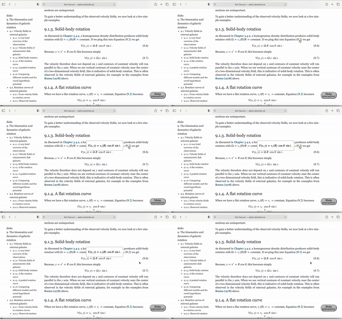
This book uses MathJax to typeset math and equations, with some customizations from the basic setup. The different pages contain links to equations on different webpages, but be aware that clicking on them will load the entire new webpage (which may take a while) and only go to the correct equation at the end of the loading (which is when MathJax can resolve the reference). This means that if you have made the page interactive, clicking on an equation link on another page without choosing to open the link in a new page will sever your interactive session (the same holds for links to other sections and chapters). To make seeing referenced equations easier, hovering over the equation link will bring up a tooltip window that displays the equation, as shown in the example below

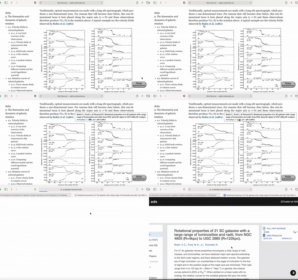
References can also be viewed by hovering over the reference, which further allows you to click on the links to follow the reference to its source, as shown in the next example.

In the references, the journal title is linked to the DOI (which typically leads to the journal version, except for very old papers), the volume to the ADS entry, and the page numbers to the arXiv version, when they exist. Clicking on a reference brings you to its entry in the References chapter.

You can similarly hover over figure references to bring up a tooltip that displays the figure and its caption (note that this type of hovering is turned off for figure references right next to the target figure). And you can hover over Section and Chapter references to show a tooltip window with a preview of the linked Section/Chapter as well!

The notes use a combination of HTML, CSS, and Javascript. Some of the included Javascript code interferes badly with the MathJax library for typesetting the math. This is known to happen in particular in the Safari browser. The notes are best viewed in Chrome, because they are developed in Chrome; other browsers may work too, but if you are having problems, try viewing them in Chrome.

← Previous section Next section →