
10.3. The velocity distribution in the solar neighborhood
We can now use the axisymmetric Jeans equation and the distribution function models for disks that we have looked at in this chapter so far to attempt to understand the kinematics of stars in the solar neighborhood. We will focus here on the kinematics of stars near the Sun in the mid-plane of the disk, with velocities \((v_R,v_\phi)\).
10.3.1. The asymmetric drift and the Sun’s motion
We start by using the axisymmetric, radial Jeans equation to understand the overall properties of the observed velocity distribution of different populations of stars. We measure the velocities of nearby stars by determining how fast stars move with respect to the Sun, either as the line-of-sight velocity measured as a Doppler shift or as the proper motion of a star on the sky. (Note that we directly observe the velocity with respect to the Earth [or with respect to a satellite, when making observations from space], but we know the Earth’s [or satellite’s] velocity well enough that we can correct measured velocities for the Earth’s motion; typically velocities are correct to the Solar system barycenter rather than to the Sun, but for galactic purposes the difference between these reference frames does not matter]. The axisymmetric Jeans equation applies to velocities in the Galactocentric coordinate frame, so to use them we need to correct for the Sun’s motion with respect to this frame. The Sun’s motion, however, is not known at high precision and some of the best constraints on it actually come from applying the axisymmetric Jeans equation.
As discussed in Appendix A.3, we can convert observed velocities to the Galactic coordinate system, where velocities are commonly denoted as \((U,V,W)\) (these are the velocities in the Cartesian coordinate system of Galactic coordinates centered on the Sun). Because any observed star is not located exactly at the Sun’s location, we cannot, after accounting for the Sun’s motion, directly interpret \(U\) as minus the Galactocentric radial velocity or \(V\) as the Galactocentric azimuthal velocity as required by the axisymmetric Jeans equation. However, for stars that are close to the Sun, the difference is small and, moreover, we can use the Oort constants to correct a star’s velocity for the difference between a star’s position and the Sun’s position. Remember that the Oort constants, which we introduced in Chapter 8.4, describe the velocity field as a function of distance from the Sun to first order in the distance; using the measured Oort constants we can thus correct observed velocities for the effect of differential Galactic rotation to what they would be if observed at the exact position of the Sun. This is most easily done at the level of the observed proper motions and line-of-sight velocities which get corrected as (see Equations 8.38, 8.39, and 8.40) \begin{align} v_\mathrm{los}(D,l) & \rightarrow v_\mathrm{los}(D,l) - D\,\left[K + A\,\sin 2l + C\,\cos 2l\right]\,\cos b\,,\\ \mu_l(D,l) & \rightarrow \mu_l(D,l)-\left(B + A\,\cos 2l - C\,\sin 2l\right)\,\cos b\,,\\ \mu_b(D,l) & \rightarrow \mu_b(D,l)+\left(K + A\,\sin 2l + C\,\cos 2l\right)\,\sin b\,\cos b\,. \end{align} We then compute \((U,V,W)\) from the corrected velocities. Overall, this is a small correction for local stars and is therefore not that important, but it becomes more important when the distance increases. Typical random velocities of stars in the disk near the Sun are \(\gtrsim 10\,\mathrm{km\,s}^{-1}\); at a distance of 100 pc, this corresponds to a proper motion of \(100\,\mathrm{km\,s}^{-1}\,\mathrm{kpc}^{-1} \approx 20\,\mathrm{mas\,yr}^{-1}\) (because \(1\,\mathrm{mas\,yr}^{-1} \approx 5\,\mathrm{km\,s}^{-1}\,\mathrm{kpc}^{-1}\)). From the measured values of the Oort constants (see Chapter 8.4), the maximum correction in \(\mu_l\) is \(|A-B| \approx 27\,\mathrm{km\,s}^{-1}\,\mathrm{kpc}^{-1} \approx 5.5\,\mathrm{mas\,yr}^{-1}\) and the maximum correction in \(\mu_b\) is even smaller. The correction is therefore much smaller than the typical random motion.
We can then re-write the Stromberg asymmetric drift Equation (10.8) in terms of \(U\) and \(V\), assuming that the Milky Way is axisymmetric and therefore \(\overline{v_R^2} = \sigma_R^2 = \sigma_U^2\) and \(\overline{v_R v_z} = \sigma_{UW}^2\) \begin{equation}\label{eq-stromberg-obs} -\overline{V}-V_0 = \frac{\sigma_U^2}{2\,v_c}\,\left[\frac{\sigma_V^2}{\sigma_U^2}-1-\frac{\partial \ln [\nu\,\sigma_U^2]}{\partial \ln R} -\frac{R}{\sigma_U^2}\,\frac{\partial \sigma^2_{UW}}{\partial z}\right] \,. \end{equation} From the fact that the planar and vertical components of the orbital motion are approximately decoupled for disk orbits, we expect \(\sigma_{UW}^2\) to vanish. Observations of the full velocity distribution indeed show that this is the case (see below). Everything in the equation above is then directly observable, except for \(V_0\) and \(v_c\).
The solar neighborhood consists of stars with ages between zero and about 12 Gyr. Because of interactions with, for example, molecular clouds and spiral structure, older stars have larger velocity dispersions \(\sigma_U\). From Equation (10.28), it is clear that they will have a different value of \(-\overline{V}-V_0\). The two main unknowns in Equation (10.28), \(V_0\) and \(v_c\), should be the same no matter what population we use to determine them (at least if the Milky Way is axisymmetric, which was the main assumption behind Equation 10.28). Therefore, we can use the kinematics of different populations of stars to determine \(V_0\) and \(v_c\).
Using Equation (10.28) to determine \(V_0\) and \(v_c\) from a single population of stars is difficult, because it requires measuring all of the terms within square brackets. The second of these involves the radial gradient of the density and of the velocity dispersion, which are difficult to determine from a local sample of stars. People have therefore attempted to get around measuring the factor in square brackets, by considering the observed relation between \(\overline{V}\) and \(\sigma_U^2\). If it appears that there is a simple relation between these two quantities, then we could parameterize this relation and essentially fit for the value of the square brackets. However, proceeding along this line means that we lose the ability to determine \(v_c\), because it is degenerate with the quantity in square brackets if we do not directly measure the quantity in square brackets. Because much interesting dynamics can be done in the solar neighborhood, but this requires one to correct for the Sun’s motion, only determining \(V_0\) is still very interesting.
Dehnen & Binney (1998b) performed this type of measurement using the Hipparcos data (HIPPARCOS Collaboration 1997). Hipparcos was a satellite similar to the more recent Gaia satellite and Hipparcos observed about 120,000 stars over a few years around 1990 to measure their parallaxes and proper motions. Line-of-sight velocities were not available for the stars in the sample selected by Dehnen & Binney (1998b), so they had to deproject. This deprojection is possible for a sample surrounding the Sun, because each proper motion measurement gives a different projection of the same three-dimensional velocity distribution. They measured \(\overline{V}\), as well as \(\overline{U}\) and \(\overline{W}\) which in an axisymmetric Galaxy should simply reflect the Sun’s motion: \(\overline{U} = -U_0\) and \(\overline{W} = -W_0\), because \(\overline{v_R} = \overline{v_z} = 0\). They performed this measurement for different samples of stars along the main sequence selected using the \(B-V\) color, which is correlated with the mean age of the population.
Figure 10.4 displays their basic measurements of \(-\overline{V}\), \(-\overline{U}\), and \(-\overline{W}\) versus \(B-V\) in the left-hand panel (they display minus the mean, because this is directly equal to the Sun’s motion for \(U\) and \(W\) and equal to the Sun’s motion for \(\sigma_U = 0\) for \(V\)). The right-hand panel shows the same measurements, but plotted against \(S^2\), which is a measure of the velocity dispersion squared (\(S^2 \propto \sigma_U^2\), but not equal; this was a convenient quantity to determine in the process of deprojecting the proper motions).
|
|
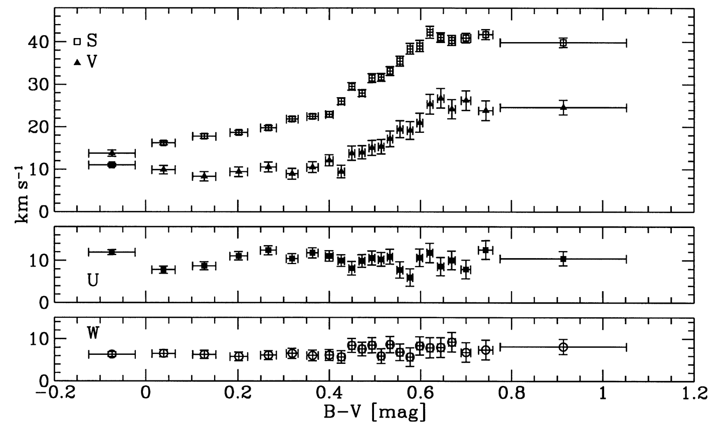
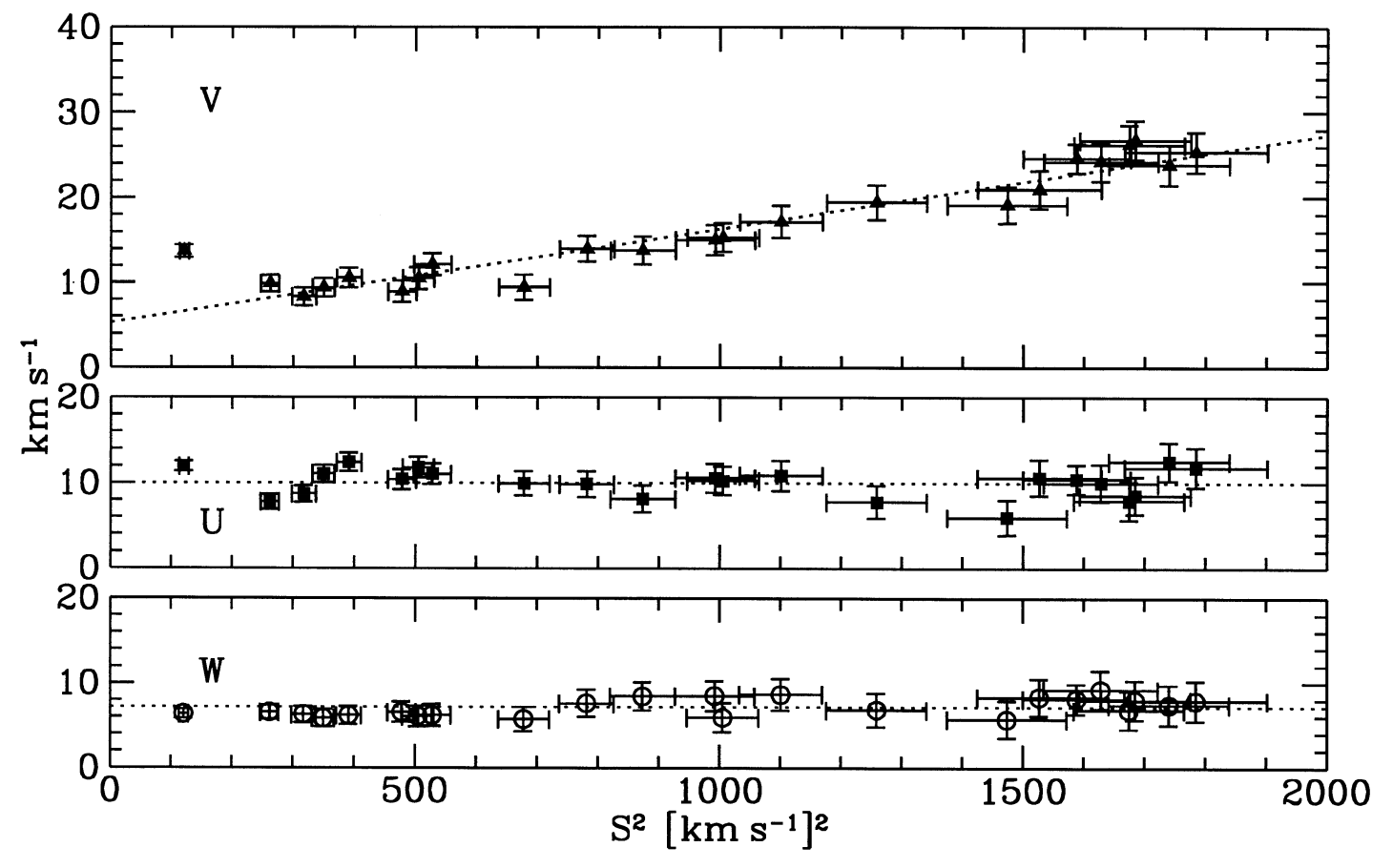
Figure 10.4: Mean velocities in \(U\), \(V\), and \(W\) and total velocity dispersion \(S\) as a function of color (left panel) and the same mean velocities vs. the total velocity dispersion \(S\) in the solar neighborhood (right panel) in the solar neighborhood (Dehnen & Binney 1998b).
As expected, there is no trend with \(B-V\) in \(-\overline{U}\) and \(-\overline{W}\) and we can combine the measurements from each population to estimate \(U_0\) and \(W_0\). This gives
\begin{equation} U_0 = 10.00\pm 0.36\,\mathrm{km\,s}^{-1}\,;\quad W_0 = \phantom{1}7.17\pm0.38\,\mathrm{km\,s}^{-1}\,, \end{equation}
The measurement of \(-\overline{V}\) does display a trend with \(B-V\). From the left-hand panel, it is clear that \(\overline{V}\) and \(S^2\) trace each other, as expected from the asymmetric drift equation in the form of Equation (10.28) and this is borne out in the right-hand panel. From the right-hand panel, it appears that there is a linear relation between \(\overline{V}\) and \(S^2\). This type of relation would make sense from Equation (10.28) if the quantity in the square brackets does not depend on \(B-V\), that is, if it is the same for all stellar populations. This would appear to be a reasonable assumption: the ratio \(\sigma_V^2/\sigma_U^2 = B/(B-A)\) in the epicycle approximation and does not vary much as the velocity dispersion increases; similarly, it is not unreasonable to assume that stars have similar density distribution \(\nu(R)\) and dispersion profiles \(\sigma_U(R)\), such that the derivative in the second term should not vary much. Therefore, if we assume that the quantity in square brackets is constant, then we can fit for a linear relation between \(-\overline{V}\) and \(S^2\) and the intercept at \(S^2 = 0\) of this relation will be equal to \(V_0\). This is the fit that is shown as a dotted line in the figure above and it gives \(V_0 = 5.25\pm0.62\,\mathrm{km\,s}^{-1}\).
Even though there clearly seems to be a linear relation between \(\overline{V}\) and \(\sigma_U^2\), this linear relation is likely spurious and leads to an incorrect value of \(V_0\). This is because according to our current best understanding of the structure of the Milky Way’s disk, the quantity in square brackets in Equation (10.28) is not constant, but is different for different stellar populations. In particular, we now know that the Milky Way disk consists of a large number of populations with very different spatial densities. These densities \(\nu(R,z)\) are different enough to make a large difference in the quantity in square brackets.
A good illustration of this point is given by the decomposition of the Milky Way’s stellar surface density into stellar populations separated by age, metallicity, and alpha-enhancement by Mackereth et al. (2017) (see Chapter 11 for a discussion of the metallicity and alpha-enhancement of stars). This is shown in Figure 10.5.
![Figure 6 from Mackereth et al. (2017): Disk surface density distributions of stellar populations separated by [a/Fe], [Fe/H], and age Sun](../_images/mackereth17_figure6.png)
Figure 10.5: Surface density profiles of stellar populations separated by age, metallicity, and [\(\alpha\)/Fe] (Mackereth et al. 2017).
The first thing to notice is that many populations do not look like simple exponential distributions, but instead have a radius at which the surface density peaks (first discovered by Bovy et al. 2016). Secondly, while for older, low-[\(\alpha\)/Fe] and for high-[\(\alpha\)/Fe] stars the surface density is declining around \(R_0 = 8\,\mathrm{kpc}\), for many of the younger populations the peak in the surface density is at \(R > R_0\) and the surface density near the Sun is increasing for these populations. As we discussed in Section 10.2.2.1 above, this behavior leads to a negative asymmetric drift (that is, \(\overline{v_\phi} > v_c\) as opposed to the “normal” \(\overline{v_\phi} < v_c\) behavior). It is clear that this type of behavior wreaks havoc on efforts to approximate Stromberg’s asymmetric drift equation as a linear relation between \(\overline{V}\) and \(\sigma_U^2\)!
This effect was first pointed out by Schönrich et al. (2010), by looking at the relation between \(\overline{V}\) and \(\sigma_U^2\) in a model for the Milky Way disk that includes chemical evolution and the growth and kinematics of different stellar populations (developed by Schönrich & Binney 2009). Figure 10.6 displays the relation between \(-\overline{V}\) and \(\sigma_U^2\) in this model, which has \(V_0 = 0\) as the green squares:
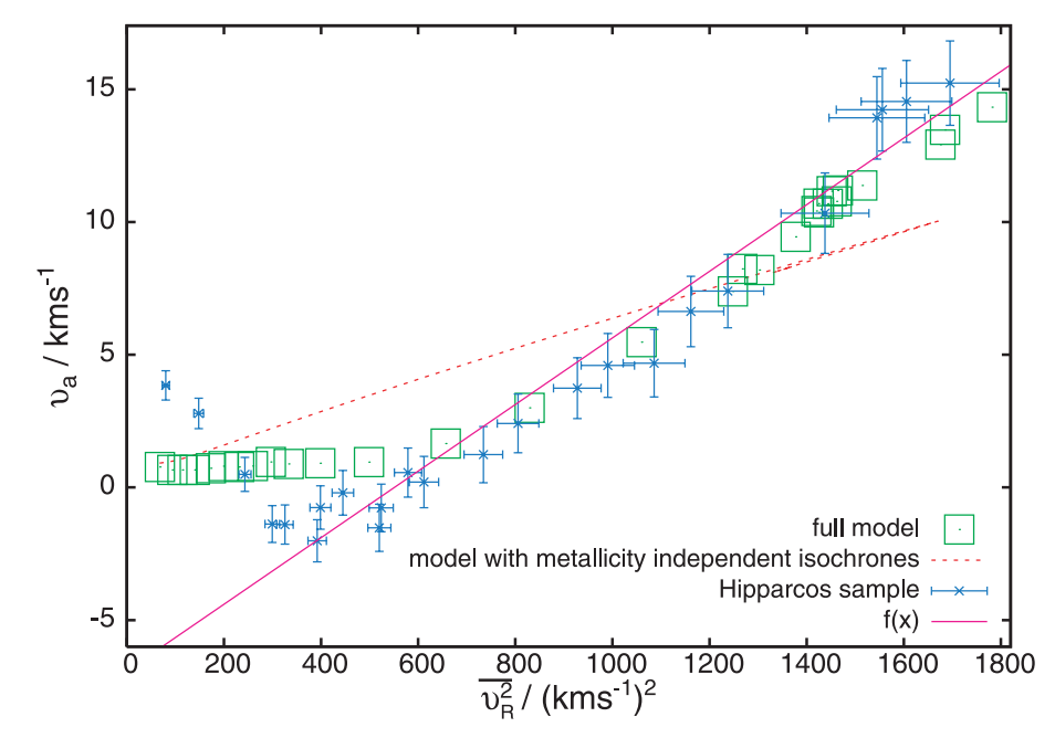
Figure 10.6: Asymmetric drift in the solar neighborhood in a realistic chemical evolution model (Schönrich et al. 2010).
A version of the Hipparcos results is included as the blue points with errorbars (these points are shifted by \(V_0 = 11\,\mathrm{km\,s}^{-1}\) to better agree with the model). At large values of \(\sigma_U^2\), the model follows the same type of linear relation as the model, but at small values of \(\sigma_U^2\) the model has a constant value of \(\overline{V}\). This is because the populations that have small \(\sigma_U^2\) are the populations which have a density profile that is flat or increasing near the Sun, and such populations have a small asymmetric drift or even a slightly negative one.
To see how this happens in a simple model, we can use the Dehnen distribution functions from Section 10.2.2.3 above to simulate stellar populations in the solar neighborhood. We simulate 25 populations with \(\sigma_R(R_0)/v_c\) between \(0.01\) and \(0.2\) (that is, \(\sigma_R(R_0)\) ranging from \(\approx 2\,\mathrm{km\,s}^{-1}\) to \(\approx 45\,\mathrm{km\,s}^{-1}\)) in a potential with a flat rotation curve. We assume that every
population has \(\sigma_R(R) = \sigma_R(R_0)\,e^{-R/R_0}\) and that \(\Sigma(R) \propto e^{-R/h_R}\). We then consider two cases: (i) \(h_R = R_0/3\) for all populations (thus, the scale length is \(\approx 2.7\,\mathrm{kpc}\), a reasonable value for stars in the disk of the Milky Way), and (ii) the scale length transitions from \(h_R = R_0/3\) at large \(\sigma_R\) to \(h_R = -R_0/3\) at small \(\sigma_R\) (we transition the scale length with a tanh function
of \(1/h_R\) to go through a flat profile around \(\sigma_R^2 = 500\,\mathrm{km}^2\,\mathrm{s}^{-2}\)). The result is shown in Figure 10.7.
[9]:
from galpy.df import dehnendf
vo= 220. # to scale velocities to km/s
srs= numpy.linspace(0.01,0.2,25)
# First do case where h_r = 1./3. everywhere
hrs= 1./3.*numpy.ones_like(srs)
vas_hrconst= numpy.empty_like(srs)
for ii,(sr,hr) in enumerate(zip(srs,hrs)):
    df= dehnendf(profileParams=(hr,1.0,sr),beta=0.)
    vas_hrconst[ii]= 1.-df.meanvT(1.)
figure(figsize=(7.5,4))
line_hrconst= plot(srs**2.*vo**2.,vas_hrconst*vo,'o',
                   label=r'$h_R = R_0/3$')
# Now do case where h_r varies
hrs= 1./(numpy.tanh((srs-0.1)/0.008)*3)
hrs[srs > 0.1]= 1./(numpy.tanh((srs[srs > 0.1]-0.1)/0.05)*3)
vas_hrtrend= numpy.empty_like(srs)
for ii,(sr,hr) in enumerate(zip(srs,hrs)):
    df= dehnendf(profileParams=(hr,1.0,sr),beta=0.)
    vas_hrtrend[ii]= 1.-df.meanvT(1.)
line_hrtrend= plot(srs**2.*vo**2.,vas_hrtrend*vo,'s',
    markerfacecolor='none',
    label=r'$1/h_R = \mathrm{between}\ -3/R_0\ \&\ 3/R_0$')
xlabel(r'$\sigma_R^2\,(\mathrm{km}^2\,\mathrm{s}^{-2})$')
ylabel(r'$v_c-\overline{v_\phi}\,(\mathrm{km\,s}^{-1})$')
xlim(-1.,1850.)
ylim(-6.,19.99)
legend(handles=[line_hrconst[0],line_hrtrend[0]],
       fontsize=17.,loc='upper left',frameon=False);

Figure 10.7: Asymmetric drift in the solar neighborhood in a model where colder stellar populations have rising surface-density profiles.
When the scale length is constant, we get the expected linear behavior between the asymmetric drift and the velocity dispersion squared. But when the scale length is variable and becomes negative (corresponding to an increasing density for those populations near the Sun), we see that we get the same behavior as in the complicated chemical-evolution model discussed above: the asymmetric drift becomes slightly negative around zero once the radial density becomes flat or increasing at the solar circle.
By adjusting the solar motion component \(V_0\) in their chemical evolution model, Schönrich et al. (2010) found a best-fit between their model and the observed kinematics of stars in the solar neighborhood for \begin{equation} V_0 = 12.24\pm0.47\,\mathrm{stat.}\,\pm2\,(\mathrm{syst.})\,\mathrm{km\,s}^{-1}\,, \end{equation} with a significant contribution from systematics related to the complexity of the velocity distribution (see below).
The asymmetric drift, while a simple consequence of the equilibrium dynamics of stellar disks, therefore manifests itself in complicated ways in galactic disks. This is because of its dependence on the radial profile of the density of stellar populations, which has complicated trends for different populations due to the complex formation and evolution history of galactic disks.
10.3.2. The distribution of velocities in the solar neighborhood
The discussion of the kinematics of stars in the solar neighborhood so far has focused solely on the behavior of the mean velocity in different directions, using the axisymmetric, radial Jeans equation to provide the equilibrium interpretation. But we have sufficient data on velocities of stars in the solar neighborhood to investigate the full three-dimensional distribution of velocities and compare it to the predictions from the equilibrium distribution function models in Section 10.2.
The first unbiased determinations of the three-dimensional velocity distribution of stars near the Sun was made possible by observations taken with the Hipparcos satellite and we are now able to look at this distribution in more detail with data from the Gaia satellite. What we learned about the in-plane velocity distribution from Hipparcos has been confirmed by Gaia observations, but Gaia has revealed previously-unseen structure in the vertical phase-space distribution that is relevant to understanding the Solar neighborhood’s vertical dynamical state. In this section, we first focus on the in-plane velocity distribution, that is, the distribution of \((U,V)\) (which many of the authors mentioned below will often denote as \((v_x,v_y)\)) and then we show how Gaia changed our understanding of the vertical phase-space distribution.
Before looking at the measured velocity distribution, we use a Dehnen distribution function from Section 10.2.2.3 above to predict the in-plane distribution that we should see for an equilibrium, axisymmetric disk. From the discussion in Section 10.2.2.1, we know that for close-to-circular orbits, all of the distribution functions that we discussed above will be approximately Gaussian. But let’s look at the velocity distribution for a population of stars with \(\sigma_R(R_0) = 30\,\mathrm{km\,s}^{-1}\), a value appropriate for the few Gyr old stars in the solar neighborhood that make up the bulk of the Hipparcos sample (for simplicity, we again assume \(\Sigma(R) \propto e^{-R/h_R}\) with \(h_R = R_0/3\) and \(\sigma_R(R) \propto e^{-R/R_0}\), and we use a flat rotation curve). This is shown in Figure 10.8.
[10]:
from galpy.df import dehnendf
vo= 220. # to scale velocities to km/s
sr= 30./vo
df= dehnendf(profileParams=(1./3.,1.0,sr),beta=0.)
vRmin, vRmax= -120./vo,120./vo # vR = -U
vTmin, vTmax= 1.-120./vo, 1.+60./vo # vT, not V
nvR= 101
nvT= 102
vRs= numpy.linspace(vRmin,vRmax,nvR)
vTs= numpy.linspace(vTmin,vTmax,nvT)
vdf= numpy.empty((nvR,nvT))
for ii,vR in enumerate(vRs):
    for jj,vT in enumerate(vTs):
        vdf[ii,jj]= df(numpy.array([1.,-vR-10./vo,vT+12.24/vo]))
figure(figsize=(5,5))
galpy_plot.dens2d(vdf.T,origin='lower',cmap='gist_yarg',
                  xlabel=r'$U\,(\mathrm{km\,s}^{-1})$',
                  ylabel=r'$V\,(\mathrm{km\,s}^{-1})$',
                  contours=True,cntrmass=True,gcf=True,
                  levels=numpy.array([2,6,12,21,33,50,68,
                                      80,90,95,99,99.9])/100.,
                  cntrcolors=['0.9','0.8','0.7','0.6','0.5',
                              '0.4','0.3','0.2','0.1','0.',
                              'k','k'],
                  xrange=[(-vRmax-0.5*(vRs[1]-vRs[0]))*vo,
                          (-vRmin+0.5*(vRs[1]-vRs[0]))*vo],
                  yrange=[(vTmin-0.5*(vTs[1]-vTs[0])-1.)*vo,
                          (vTmax+0.5*(vTs[1]-vTs[0])-1.)*vo]);

Figure 10.8: Planar velocity distribution in the solar neighborhood in a Dehnen distribution function model.
The contour levels here contain (2, 6, 12, 21, 33, 50, 68, 80, 90, 95, 99, and 99.9) % of the distribution and are the same as those in the observational determinations below. We have also shifted the velocity distribution to heliocentric coordinates using the solar motion discussed in the previous section.
The properties and shape of this distribution are as expected. Overall, the distribution is close to Gaussian and is symmetric around the \(v_R = 0\) line (which falls at \(U = -10\,\mathrm{km\,s}^{-1}\) in heliocentric coordinates). The effect from the asymmetric drift shifts the peak away from \(v_\phi = v_c\) and causes the \(V\) distribution to be skewed: the velocity distribution extends to much more negative values of \(V\) than it extends to positive values. The velocity distribution is smooth. Even when we mix multiple populations with different values of \(\sigma_R(R_0)\) and/or \(\Sigma(R)\) and \(\sigma_R(R)\), we would still expect a similar shape, with similar smoothness. Observationally, the properties of the local velocity distribution are sometimes summarized using the velocity ellipsoid, which is its covariance matrix \begin{equation}\label{eq-diskequil-velellipsoid} \left(\begin{matrix} \sigma_R^2 & \sigma_{R\phi}^2 & \sigma_{Rz}^2 \\ \sigma_{R\phi}^2 & \sigma_\phi^2 & \sigma_{\phi z}^2\\ \sigma_{Rz}^2 & \sigma_{\phi z}^2& \sigma_z^2\end{matrix}\right) = \left(\begin{matrix} \sigma_U^2 & \sigma_{UV}^2 & \sigma_{UW}^2 \\ \sigma_{UV}^2 & \sigma_V^2 & \sigma_{VW}^2\\ \sigma_{UW}^2 & \sigma_{VW}^2& \sigma_W^2\end{matrix}\right)\,, \end{equation} where the right-hand side holds in the solar neighborhood, but the left-hand side is the general form. Because a covariance matrix describes an ellipsoidal shape, the off-diagonal components are generally expressed as angles representing the angles of this ellipsoid with respect to the coordinate axes; The angle \(l_V\) associated with \(\sigma_{R\phi}^2\) is the vertex deviation and is given by \begin{equation}\label{eq-diskequil-vertexdeviation} \tan \left( 2\,l_V\right) = 2\,\frac{\sigma^2_{R\phi}}{\sigma_R^2-\sigma_\phi^2}\,. \end{equation} The angle associated with \(\sigma_{Rz}^2\) is the tilt of the velocity ellipsoid and is discussed in further detail in Section 10.4.1 below. The steady-state, axisymmetric prediction is that the vertex deviation is equal to zero: \(l_V = 0\) and \(\sigma_{R\phi}^2 = 0\).
Figure 10.9 displays the observed velocity distribution, as determined by Dehnen (1998) from Hipparcos data and by Gaia Collaboration et al. (2018) using the more recent Gaia data:
|
|
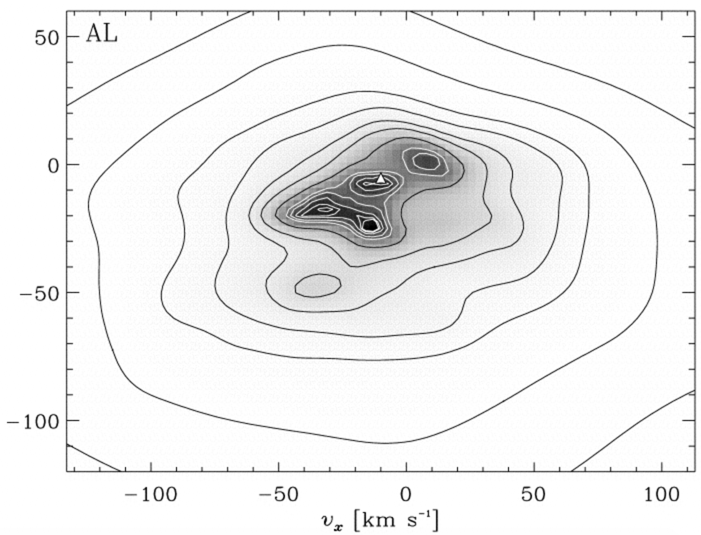
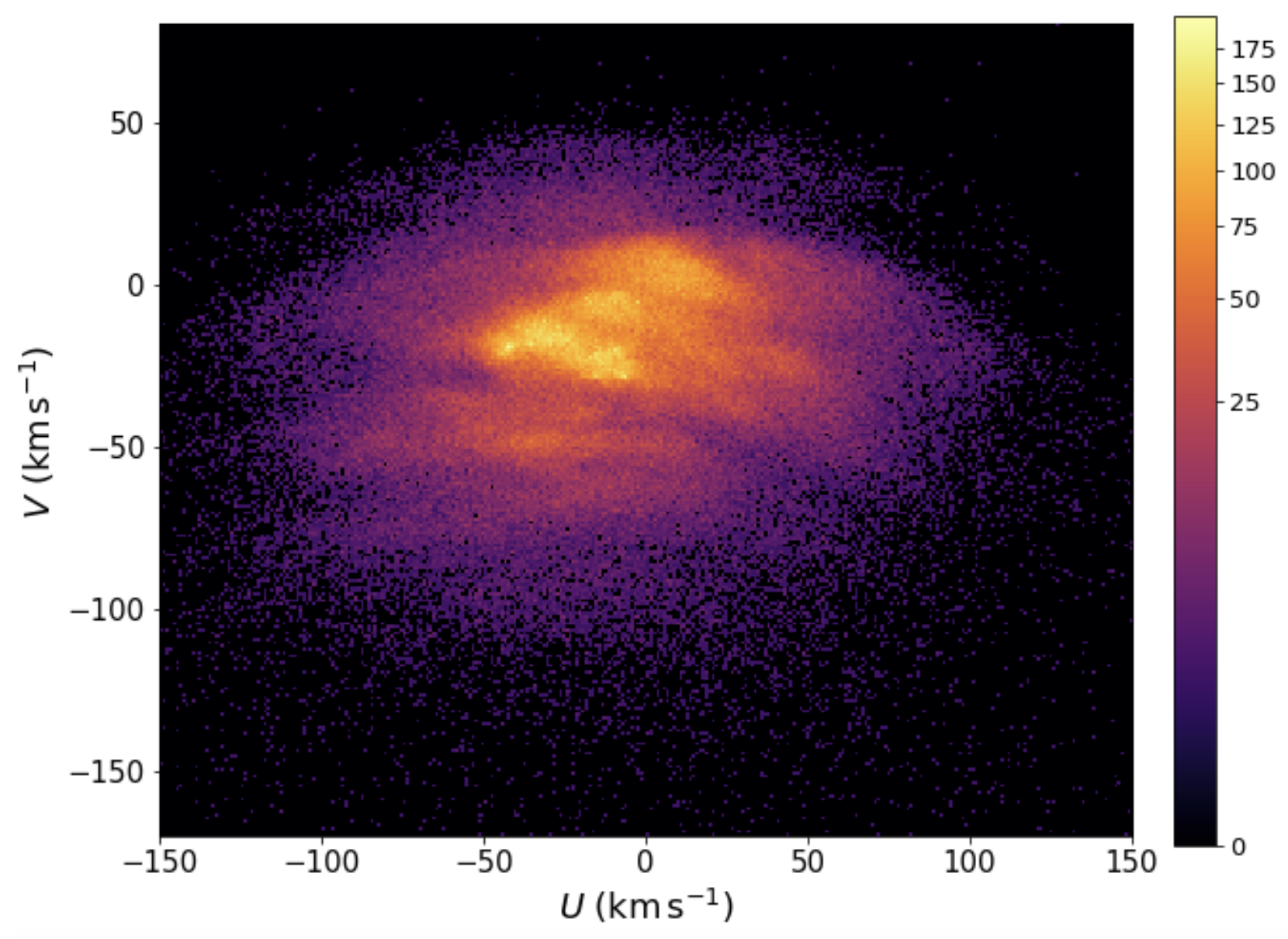
Figure 10.9: Observed planar velocity distribution in the solar neighborhood from Hipparcos (left: Dehnen 1998) and from Gaia (right: Gaia Collaboration et al. 2018).
We see that this distribution is quite different from that expected for an equilibrium, axisymmetric disk: rather than being a smooth distribution that is symmetric around \(v_R = 0\), the distribution is characterized by many overdensities and a vertex deviation of \(l_V \approx 10^\circ\). Because Hipparcos only measured proper motions, Dehnen (1998) had to deproject the velocity distribution and this makes it difficult to interpret the significance of all of the features in the observed velocity distribution, but the Gaia data beautifully confirm that the main overdensities are real and that they, in fact, have further small-scale structure. Most of the structures seen in the velocity distribution—which are known as moving groups—had been known before Hipparcos from previous determinations of the velocity distribution (e.g., Boss 1908; Hertzsprung 1909; Roman 1949; Ogorodnikov & Latyshev 1968; Eggen 1970), but it had not been clear how prominent they were until the Hipparcos results. Bovy et al. (2009) find that about 40% of local stars are contained in the main moving groups. This is a very significant number of stars!
The vertical velocity distribution revealed by Hipparcos was unremarkable: roughly symmetric between positive and negative velocities and with an approximate Gaussian shape. However, investigations of the vertical density and velocity distribution using data from large pre-Gaia surveys demonstrated the existence of mean-vertical-velocity gradients (Siebert et al. 2011; Williams et al. 2013) and vertical-density asymmetries (Widrow et al. 2012; Xu et al. 2015) that complicated this picture. Gaia’s second data release (DR2) then definitively showed the existence of a spiral-shaped vertical phase-space perturbation, known as the Gaia phase-space spiral (Antoja et al. 2018), whose projection into the vertical density manifests itself as a density wave (Bennett & Bovy 2019) and whose radial behavior leads to mean velocity gradients. In the Gaia DR2 data, the phase-space spiral was most obvious when color-coding the vertical phase-space distribution by average rotation velocity, but in the early third data release data the spiral strongly stands out as a density contrast as well as shown in Figure 10.10.
|
|
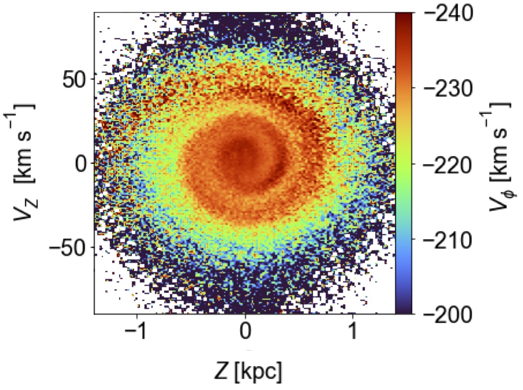
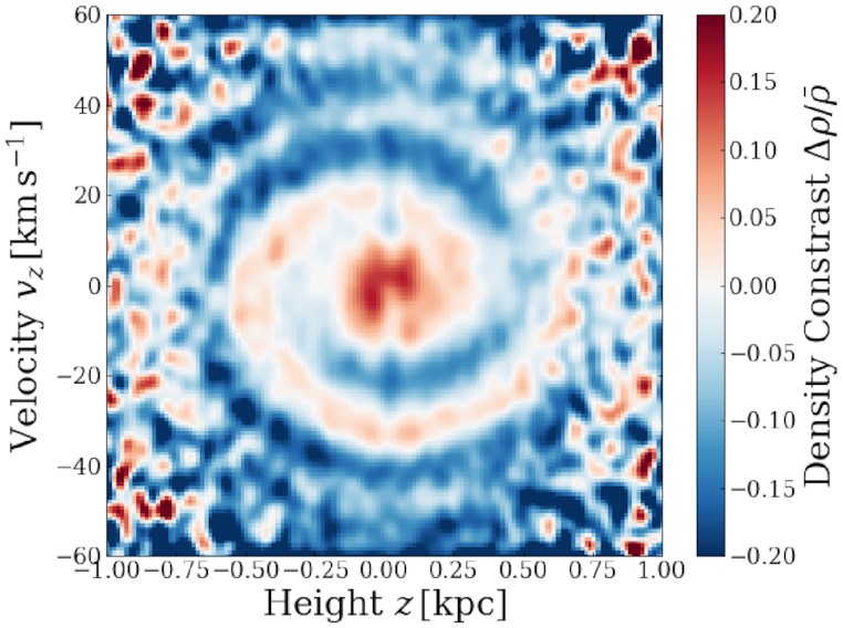
Figure 10.10: The local vertical phase-space distribution color-coded by mean rotational velocity (left; Antoja et al. 2023) and after dividing a smooth model for the phase-space density (right; Frankel et al. 2023). A spiral perturbation can be clearly seen in both.
As Figure 10.10 demonstrates, the vertical perturbation is at the level of 10%. Because the period of orbits depends on their typical vertical height and their mean rotational velocity, this spiral cannot be an equilibrium feature and deviations from equilibrium become important when attempting to constrain local dynamical parameters to a level better than \(\approx 10\%\).
The observed velocity distribution, with its prominent moving groups and vertical phase-space spiral, is therefore very different from that expected for a steady-state galaxy. Because the moving groups contain many stars and those stars have a wide range of ages and metallicities (e.g., Famaey et al. 2005; Bensby et al. 2007; Bovy & Hogg 2010), it is very unlikely that they are clusters of stars born together that are still in the process of becoming a phase-mixed, equilibrium population (De Simone et al. 2004). They are most likely due to the effect of time-dependent, non-axisymmetric perturbations to the Galactic potential, such as those from the bar and spiral structure (e.g., Dehnen 2000; De Simone et al. 2004; Hunt et al. 2019). The most obvious cause of the phase-space spiral is a recent impact from, e.g., the Sagittarius dwarf galaxy (Antoja et al. 2018), but simulations based on its orbit cannot quantitatively explain the properties of the phase-space spiral (Bennett & Bovy 2021; Bennett et al. 2022) and its origin is therefore still a mystery.

 .
. .
. .
.