
18.4. Galaxy scaling relations
The wide range of galaxy types and galaxy properties discussed in the previous section might lead one to think that there is little order in the realm of galaxies. However, this is not true and, in fact, the galaxy population is highly regular in many respects. Nothing makes this clearer than the existence of various galaxy scaling relations, the gist of which is that the overall dynamical and stellar-population properties of galaxies only occupy a very low-dimensional sub-space in the high-dimensional space of dynamical, photometric, and morphological properties.
The important galaxy scaling relations were established in the 1970s and 1980s. All galaxy scaling relations demonstrate that a remarkably tight correlation exists between two or more a priori unrelated galaxy properties. Typically, the properties involved are a dynamical one, which thus depends on the galaxy’s dark-matter content, and a purely stellar or baryonic property. Broadly, galaxy scaling relations have had the following major uses:
As distance indicators: the most important galaxy scaling relations relate a distance-dependent quantity, such as the luminosity, to a distance-independent quantity. A calibrated relation can then be used to determine distances to galaxies by measuring the distance-independent property and using the relation to infer the distance.
As probes of the structure and evolution of the galaxy population: Galaxy scaling relations have a remarkably-small scatter around a mean trend. The mean trend with small scatter means that galaxies overall are highly regular, a regularity that requires explanation in our understanding of galaxy formation and evolution, because naively the process of galaxy formation is messy and irregular. The scatter around the mean trend contains important information about the range of internal properties of galaxies and of the evolutionary pathways that galaxies traverse.
Exactly how this plays out in practice will become clear in the examples of scaling relations that we discuss below.
At this point, galaxy scaling relations have somewhat fallen out of favor, for a variety of reasons. First of all, their usefulness as distance indicators has declined as more accurate and precise methods for galaxy distance determination have been discovered. For example, measurements of the Hubble constant \(H_0\) from the distance–velocity relation require good distances and for a while relied on galaxy scaling relations to obtain these. However, modern measurements of the Hubble constant use a distance ladder consisting of geometric distances—parallaxes to nearby stars and dynamical distances to external galaxies—Cepheid variable stars with precise distances coming from the period–luminosity relation, and type Ia supernova distances obtained using the Phillips (1993) relation (e.g., Riess et al. 2016). More reliable distances to individual galaxies that do not happen to have an observed type Ia supernova explosion can be obtained through methods such as the tip-of-the-red-giant-branch (Lee et al. 1993) or surface brightness fluctuations (Tonry & Schneider 1988; Tonry et al. 2001).
As probes for understanding galactic structure and evolution, galaxy scaling relations have been highly successful, as we will discuss below, such that the forefront of the field is now at dissecting galaxies in more detail than the broad-brush picture that emerges from scaling relations. However, the remarkable regularity of the galaxy population and the tight connection between the baryonic and dark-matter components of galaxies that scaling relations revealed is still not satisfactorily understood. New observational facilities in the next decades will be able to establish when and how scaling relations were established in the high-redshift Universe and, thus, undoubtedly lead to further progress.
The major scaling relations are separate for disk and elliptical galaxies, or better yet, rotationally-supported and dispersion-supported systems (but see Zaritsky et al. 2008). We start by discussing scaling relations for disk galaxies, the most important one of which is the Tully-Fisher relation (Tully & Fisher 1977). The Tully-Fisher relation is a tight correlation between a disk galaxy’s luminosity and a measure of the amplitude of its rotation curve. The latter is traditionally the width \(W\) of the 21 cm line in the integrated emission from the galaxy. The Doppler shifts of the 21 cm line of neutral hydrogen maps the circular velocity curve of a galaxy, because gas can be assumed to be on close-to-circular orbits (see Chapter 8.1); for a galaxy with ordered rotation with a maximum circular velocity \(V_{\mathrm{max}}\), the range of rotation velocities extends from \(-V_{\mathrm{max}}\) to \(V_{\mathrm{max}}\) and, when viewed edge-on, we then have that \(W = 2\,V_{\mathrm{max}}\). Because it only requires the integrated emission from the galaxy, the line-width \(W\) is easy to determine observationally. Figure 18.21 displays some integrated HI spectra as a function of velocity.
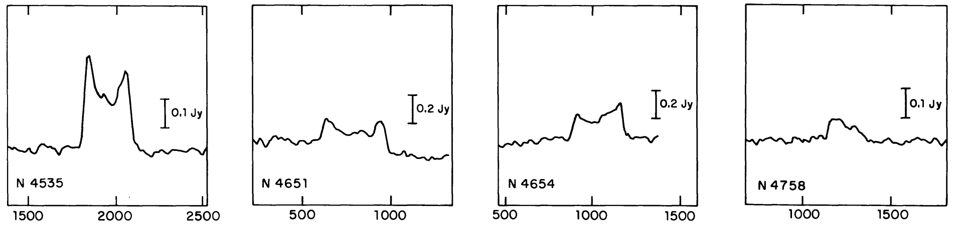
Figure 18.21: The 21cm line-width of various galaxies (Tully & Fisher 1977).
The velocity profile of the galaxy on the left, NGC 4535, is a typical example of the horn profile expected for a flat rotation curve (where most of the emission is at the plateau value of the circular velocity). It is clear from this figure that the measurement of \(W\) is not entirely unambiguous, as the profiles typically deviate from the expected mirror symmetry for well-ordered rotation.
The luminosity in the Tully-Fisher relation is that in any optical or near-infrared band, that is, bands dominated by the emission from stars. Using observations of galaxies in the Local Group and other nearby galaxy groups, Tully & Fisher (1977) found that there is a tight correlation between the luminosity \(L\) and the line width \(W\) of the form \begin{equation}\label{eq-exgal-tf-form} L \propto W^\alpha\,. \end{equation} The exponent \(\alpha\) depends on the bandpass in which the luminosity is measured and varies between \(\approx3\) to \(\approx4.5\) from blue to red bandpasses (Sakai et al. 2000). The Tully-Fisher relation is not usually presented in the form of Equation (18.29), but rather as a linear relation between the absolute magnitude \(M\) and \(\log_{10}W\), i.e., \begin{equation} M = \beta \log_{10} W + \mathrm{constant}\,, \end{equation} where then \(\beta = 2.5\alpha\). The Tully-Fisher relation calibrated using precise Cepheid distances in some of the major optical bands is shown in Figure 18.22, which clearly demonstrates the remarkably small scatter around the mean relation.
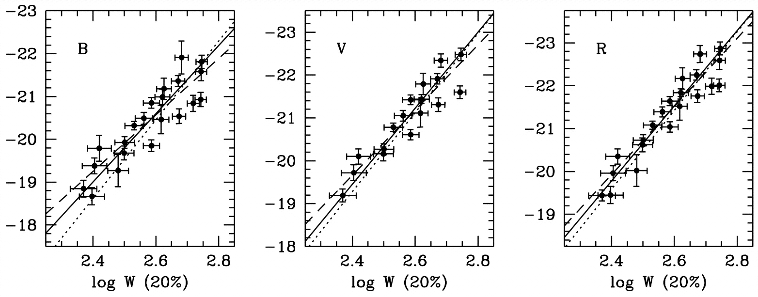
Figure 18.22: The Tully-Fisher relation (adapted from Sakai et al. 2000).
How and when a relation like the Tully-Fisher relation arises becomes clear through the following argument. Roughly, the relation between the circular velocity \(v_c\) and the enclosed mass \(M\) is \(v_c^2 = {GM / R}\). We saw in Chapter 2.3 that this relation is exact for spherical systems, which disk galaxies are not, but we saw in Chapter 7 that this relation is only off by \(\approx 15\%\) for typical disk galaxies. We then relate \(M\) and \(R\) to the luminosity \(L\) using \(M = (M/L)\,L\) and \(R \propto \sqrt{L/I_0}\), where \(M/L\) is the total mass-to-light ratio (including stars, gas, and dark matter) and \(I_0\) is the central surface brightness in linear flux units. We then find that \(v_c^2 \propto (M/L)\,\sqrt{L\,I_0}\) or \begin{equation}\label{eq-exgal-tfanalytic} L \propto {v_c^4\over (M/L)^2\,I_0}\,. \end{equation} If \(M/L\) and \(I_0\) are constant with \(L\), we then find that \(L \propto v_c^4\), similar to the observed Tully-Fisher relation (because \(W \propto v_c\)). The surface brightness is directly observable and, as we saw above, it is indeed the case that it is relatively constant at \(\mu_0 \approx 21\,\mathrm{mag\,arcsec}^{-2}\) for spiral galaxies (Freeman’s law; Freeman 1970). Deviations from the \(L \propto v_c^4\) form should then mostly come from luminosity dependence in the mass-to-light ratio. The Tully-Fisher relation in bluer bands has \(\alpha \approx 3\), and assuming a constant \(I_0\) this implies \(M/L \propto L^{1/6}\). Assuming that mass-to-light ratio variations are stellar-population driven, this implies that lower-luminosity galaxies have lower mass to light ratios in the bluer bands, indicating that they have relatively higher star-formation rates, because higher star-formation rates lead to lower \(M/L\). Redder bands that trace the overall stellar mass better have \(\alpha \approx 4\), implying little-to-no overall luminosity dependence of \(M/L\). Thus, stellar and dark matter are intimately linked in disk galaxies. This is a surprising result, given the seeming randomness of galaxy assembly and growth in the \(\Lambda\)CDM cosmological paradigm. Variations in \(M/L\) due to varying contributions from stars and dark matter to the total mass within the visible region of a galaxy do account for the scatter around the mean relation (e.g., Courteau & Rix 1999; Pizagno et al. 2007).
Because the Tully-Fisher relation appears to fundamentally be a relation between the stellar content (through \(L\)) and the total mass (through \(W\)), a more direct relation between these two is obtained by simply plotting the stellar mass \(M_*\) versus the maximum circular velocity. When doing this, McGaugh et al. (2000) noticed that the tight relation breaks down for low-mass galaxies with \(v_c \lesssim 90\,\mathrm{km\,s}^{-1}\), as shown in the left panel of Figure 18.23.
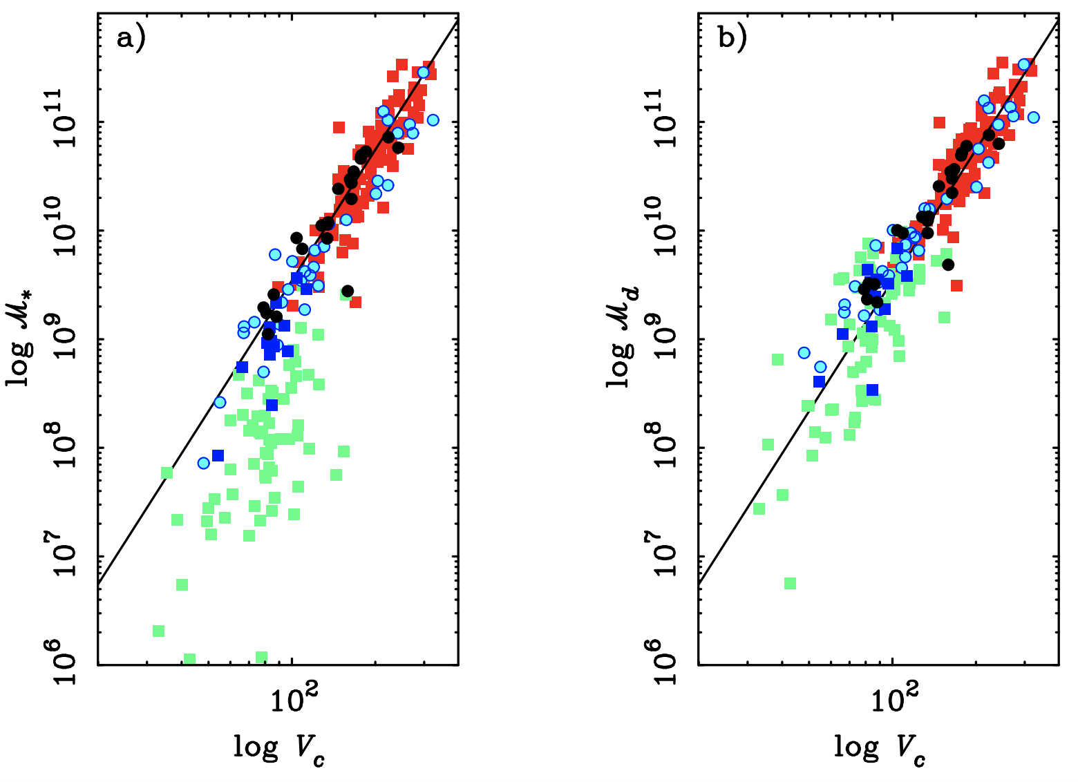
Figure 18.23: The baryonic Tully-Fisher relation (McGaugh et al. 2000).
However, they also found that a tight correlation is restored when replacing the stellar mass by the total baryonic mass \(M_b\), which includes the gas in all its phases in addition to the stars, as can be seen in the right panel of Figure 18.23. The intrinsic scatter in the relation is small: \(\approx 0.1\,\mathrm{dex}\)—about \(5\%\)—when considering \(M_b\) at a given \(v_c\) (Lelli et al. 2016b). Thus, the Tully-Fisher relation appears to fundamentally be a relation between the total baryonic mass and the total dark+baryonic mass. The breakdown of the stellar-mass–circular-velocity relation at low velocities simply reflects the increasing importance of gas in low-mass galaxies (see Chapter 1.2.2). The relation between \(M_b\) and \(v_c\) is known as the baryonic Tully-Fisher relation and the mean trend is of the form \(M_b \propto v_c^\alpha\), with \(\alpha = 3.5\) to \(4\) (McGaugh et al. 2000; Bell & de Jong 2001). Recently, a related, but slightly different statement of this relation known as the radial acceleration relation has become popular (McGaugh et al. 2016); this relation relates the acceleration due to the baryonic matter to the total acceleration due to all matter.
As we have already stressed, the existence of such a tight relation between the baryonic and total mass of a galaxy implies a close connection between the baryonic and dark-matter content in galaxies that is a priori unexpected in the \(\Lambda\)CDM paradigm. Cosmological simulations of galaxy formation recover Tully-Fisher-like relations, showing that it is an emergent property of the disk-galaxy population in \(\Lambda\)CDM that arises from the fact that the stellar mass of galaxies in simulations is proportional to the total baryonic mass within the halo’s virial radius and this, in turn, naturally correlates with the total halo mass and, thus, the circular velocity (Steinmetz & Navarro 1999). The surprising existence of the Tully-Fisher relation in part inspired the development of alternative theories of gravity, which explain the effects of dark matter by modifying the Newtonian force law rather than by introducing a new form of matter. In its most popular instance, Modified Newtonian Dynamics (MOND; Milgrom 1983b), the force law at low accelerations becomes quadratic in the acceleration \(a\), with the gravitational field \(g = a^2/a_0\), where \(a_0\) is a new constant of nature that sets the acceleration below which the acceleration transitions to this new form. For the circular acceleration \(a = v_c^2 / r\), we then find \(v_c^4 / (r^2 \,a_0) = GM/r^2\) (assuming spherical symmetry of the mass distribution), and thus, \(v_c^4 = GM\,a_0\), independent of \(r\) (Milgrom 1983a). Thus, the modified Newtonian force law both leads to flat rotation curves and a Tully-Fisher relation (for constant \(M/L\), which is more palatable in MOND, because there is no dark matter). Nevertheless, because MOND has significant trouble explaining observations of the early Universe, the late-time large-scale structure of the Universe, and the detailed internal dynamics of different types of galaxies, it is not favored by most astrophysicists. This is why we otherwise do not spend time on MOND in this book.
Like with all observational results in this chapter, the frontier of knowledge is extending the observational picture of the Tully-Fisher relation to higher redshifts to gain insight into how the relation developed and what this tells us about disk-galaxy formation. For example, Cresci et al. (2009) has found that the Tully-Fisher relation exists at \(z = 2.2\), at the time when galaxies like the Milky Way were actively forming, but with a lower normalization, showing that galaxies built up their mass in a way that preserves the slope of the Tully-Fisher relation over much of cosmic history.
A similar relation to the Tully-Fisher relation exists for elliptical galaxies: the Faber-Jackson relation (Faber & Jackson 1976). Because elliptical galaxies are supported by random motions rather than ordered rotation, the Faber-Jackson relation takes the form \begin{equation} L \propto \sigma^\alpha\,, \end{equation} where \(\sigma\) is the stellar velocity dispersion. As for the Tully-Fisher relation, the power-law exponent \(\alpha \approx 4\). Measuring the stellar velocity dispersion requires medium-resolution optical spectra, because elliptical galaxies are gas poor. The original Faber-Jackson relation is shown in Figure 18.24, which clearly shows that \(L \propto \sigma^4\) provides a good fit to the mean trend.
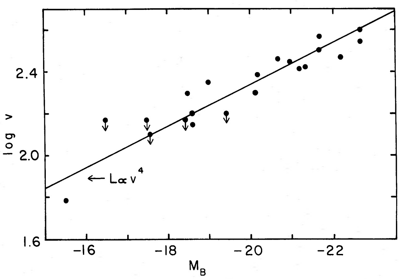
Figure 18.24: The Faber-Jackson relation (Faber & Jackson 1976).
Like for the Tully-Fisher relation, the exponent and constant of proportionality depends on the photometric bandpass used. For example, in the SDSS \(r\)-band, Bernardi et al. (2003b) report that \(\alpha = 3.91\) with an intercept of \(M_r = -19.2\) at \(\sigma = 100\,\mathrm{km\,s}^{-1}\). Across the optical bands they find that \(\alpha\) varies only between \(\approx 3.9\) and 4.
The intrinsic scatter in the Faber-Jackson relation is \(\approx 0.1\,\mathrm{dex}\), or about \(5\%\) in \(\sigma\) at a given luminosity (e.g., Nigoche-Netro et al. 2011). This is about four times bigger than the intrinsic scatter in the baryonic Tully-Fisher relation, which has only \(\approx 1\%\) intrinsic scatter in \(v_c\) at a given \(M_b\) (Lelli et al. 2016b). To reduce the scatter, research after the discovery of the Faber-Jackson relation focused on finding a third parameter that controls the scatter. Efstathiou & Fall (1984) focused on the strength of metal absorption, as traced by the depth of Mg lines, finding a relation between \(L\), \(\sigma\), and the Mg line strength. Kormendy (1977) discovered a relation between the effective radius and the central surface brightness, which is such that brighter elliptical galaxies are more diffuse than less bright galaxies. Unlike for large spiral galaxies, therefore, the surface brightness of elliptical galaxies varies systematically with their size. Because the constancy of the surface brightness was central to our understanding of how the Tully-Fisher relation appears in the \(\Lambda\)CDM paradigm, this demonstrates that surface brightness is likely another important parameter.
The crucial addition of surface brightness to the Faber-Jackson relation was done by two groups independently in two slightly different manners. Djorgovski & Davis (1987) found a relation between the effective radius \(R_e\), the central velocity dispersion \(\sigma_0\), and the mean surface brightness \(\langle I\rangle\) (in linear units) of the form \begin{equation}\label{eq-exgal-fundamental-plane} R_e \propto \sigma_0^{1.4}\,\langle I\rangle^{-0.9}\,. \end{equation} This relation is known as the fundamental plane. Simultaneously, Dressler et al. (1987) (known as the “Seven Samurai”) derived an equivalent relation, although they expressed it as a more direct modification of the Faber-Jackson relation \begin{equation} L \propto \sigma^{8/3}\Sigma_e^{-3/5}\,, \end{equation} where \(\Sigma_e\) is the average surface brightness within the effective radius. Because \(L \propto R_e^2\,\Sigma_e\) and \(\langle I\rangle \propto \Sigma_e\), their version of Equation (18.33) is approximately \begin{equation} R_e \propto \sigma_0^{4/3}\,\langle I\rangle^{-4/5}\,, \end{equation} similar to the plane found by Djorgovski & Davis (1987). They also turned their version of the fundamental plane into a powerful distance indicator for elliptical galaxies and the bulges of disk galaxies, the \(D_n - \sigma\) relation (Dressler 1987). Large samples of elliptical galaxies obtained from large surveys find a similar relation, e.g., Bernardi et al. (2003a) reports \(R_e \propto \sigma_0^{1.49}\,\langle I\rangle^{-0.75}\).
We can show that a power-law relation of the form of Equation (18.33) is expected for elliptical galaxies using similar reasoning as that which led to the expected Tully-Fisher-like relation of Equation (18.31). Because elliptical galaxies are supported by dispersion, we use the scalar virial theorem of Chapter 14.1 in the form of Equation (14.18). The scalar virial theorem relates the kinetic and potential energies. Neglecting rotation (which is small for massive ellipticals; see Section 12.1), we can simply write the scalar kinetic energy as \(K = M\sigma^2/2\). For the potential energy \(W\), we need to make an assumption about the form of the mass distribution. As often before, we approximate \(W\) as the potential energy of a homogeneous density sphere with radius \(R\), which is given by Equation (14.31): \(W = -(3/5)GM^2/R\). To account for systematic deviations from the homogeneous density sphere approximation, we write this as \(W = -f\,GM^2/R\), where \(f\) parameterizes deviations from the approximation. The scalar virial theorem then leads to \(\sigma^2 = f\,GM/R\), a relation that is quite similar to the equivalent one for spiral galaxies that we used in understanding the Tully-Fisher relation above. Following the same logic as in the derivation of Equation (18.31), we find eventually \begin{equation}\label{eq-exgal-fpanalytic} L \propto {1\over f^2\,(M/L)^2}\,\sigma^4\,\langle I\rangle^{-1}\,, \end{equation} or using \(L \propto R_e^2\,\langle I\rangle\) and approximating \(\sigma^2 \propto \sigma_0^2\), we can write this in the canonical fundamental-plane form \begin{equation}\label{eq-exgal-fpanalytic-canonical} R_e \propto {1\over f\,(M/L)}\,\sigma_0^2\,\langle I\rangle^{-1}\,. \end{equation} We see that the dependence on \(\langle I\rangle\) is approximately correct, but the predicted dependence on \(\sigma_0\) is steeper than the observed one. Thus, the combination \(f\,(M/L)\) must depend on \(\sigma_0\) to make the overall dependence on \(\sigma_0\) weaker. The deviation of the predicted fundamental plane from the observed one is know as the tilt of the fundamental plane. As we already discussed in detail in Chapter 16.2, integral-field spectroscopy (IFS) of the internal kinematics of elliptical galaxies demonstrates that this tilt is largely explained by the dependence of \(M/L\) on \(\sigma_0\) as opposed to \(f\) depending on \(\sigma_0\) (\(f\) variations are known as non-homology of the orbit distribution). In particular, detailed IFS observations find that \(M/L \propto \sigma^{0.84}\) (Equation 16.7) and plugging this into Equation (18.37), we find \begin{equation} R_e \propto {1\over f}\,\sigma_0^{1.16}\,\langle I\rangle^{-1}\,, \end{equation} which is much closer to the observed dependence of Equation (18.33). The remainder of the tilt can be explained by the non-homology of the orbit distribution.
As with the Tully-Fisher relation, current observational efforts are focused on determining the redshift evolution of the fundamental plane. The present status of these campaigns is that the fundamental plane appears similar in both power-law exponents and amplitude to the \(z\approx 0\) one out to redshift 1 (van der Wel et al. 2004; Bezanson et al. 2015) and even out to redshift 2 (van de Sande et al. 2014; Stockmann et al. 2021), although the scatter increases. This indicates that the elliptical-galaxy population undergoes relatively little evolution over the last \(\approx 10\,\mathrm{Gyr}\), with passive aging and minor mergers dominating the little evolution that exists (van Dokkum et al. 2010).

 .
. .
. .
.