← Previous section Next section →

12.1. The three-dimensional structure of elliptical galaxies and dark-matter halos

\label{sec-triaxialgrav-ellipstruct}

We briefly discussed the radial structure of elliptical galaxies and dark-matter halos in Chapter 1.2.1 and Chapter 2.4.6, but to motivate the somewhat complex methods necessary to study the mass distributions of realistic elliptical galaxies and dark-matter halos, we will start this chapter by taking a closer look at their three-dimensional structure.

The equivalent of Freeman (1970)’s discovery of the exponential nature of disk galaxies’ radial brightness profile (see Chapter 7.1), is de Vaucouleurs (1948)’s finding that the surface brightness profile of elliptical galaxies drops approximately as \(R^{1/4}\), as shown beautifully for three elliptical galaxies in Figure 21 of de Vaucouleurs (1948)’s paper, reproduced here in Figure 12.2.

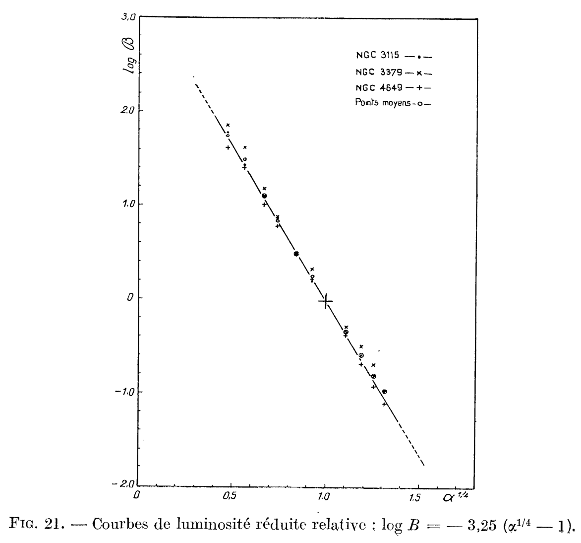
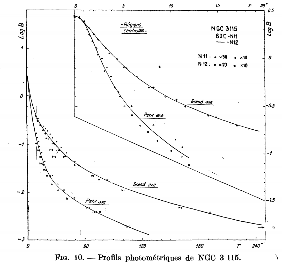
Figure 12.2: Surface brightness profile of elliptical galaxies from de Vaucouleurs (1948). The left panel shows radial profiles for NGC 3115, NGC 3379, and NGC 4549 while the right panel shows NGC 3115’s profile along the major and minor axes.

This radial profile, now known as the de Vaucouleurs profile (and even generally referred to as a “law”, even though it’s simply an observation) is given by \begin{equation}\label{eq-triaxialgrav-deVauc} I(R) = I_e\,10^{-3.33\left([R/R_e]^{1/4}-1\right)}\,, \end{equation} where the “3.33” is chosen such that half of the total luminosity is contained with \(R_e\), the effective radius. Thus, the effective radius is equal to the half-light radius, although this is only exactly true if the isophotes are circularly symmetric. It’s often more convenient to express the de Vaucouleurs profile in the form \begin{equation}\label{eq-triaxialgrav-deVauc-wexp} I(R) = I_e\,\exp\left\{-7.67\left([R/R_e]^{1/4}-1\right)\right\}\,. \end{equation} The de Vaucouleurs profile works well for the larger elliptical galaxies, but for smaller elliptical galaxies, a generalization known as the Sérsic profile is useful (Sersic 1968) \begin{equation}\label{eq-triaxialgrav-sersic} I(R) = I_e\,\exp\left\{-b_n\left([R/R_e]^{1/n}-1\right)\right\}\,. \end{equation} The constant \(b_n\) is again determined such that half of the light is within \(R_e\) and it is approximately given by \(b_n = 2\,n-0.324\) (e.g., \(b_4 = 7.676\) for the de Vaucouleurs profile; Ciotti 1991; see also Ciotti & Bertin 1999 for an improved approximation). Because the Sérsic profile becomes a pure exponential profile for \(n=1\), Sérsic profiles are able to fit photometry of disk and elliptical galaxies and smoothly interpolate between the two.

As discussed in part I, even when a galaxy or dark-matter halo is not spherical, much insight about its structure and dynamics can be gleaned from treating it as such. Because the de Vaucouleurs and Sérsic profiles provide an excellent representation of the observed surface photometry of elliptical galaxies, they are an obvious choice for building a simple spherical model for elliptical galaxies, assuming a constant mass-to-light ratio to turn the surface brightness into a surface mass density. However, the simplicity disappears once one realizes that to build a three-dimensional spherical model, one needs to de-project the two-dimensional surface mass density (e.g., using the Abel integral inversion of Equation 6.17) and, to obtain the gravitational potential and/or field, integrate over the three-dimensional density. While they are straightforward numerically, none of these operations can easily be performed analytically for either the Sérsic profile or its special de Vaucouleurs case (they can all be expressed using the “Fox H function”, a special function so special that it does not appear to be implemented in any programming language!; Baes & Gentile 2011; Baes & van Hese 2011). While precise numerical approximations for the de-projected density and mass profile exist (e.g., Vitral & Mamon 2020), often it is more convenient to approximate the surface density using a form for which the gravitational potential, field, density, and perhaps other properties such as the ergodic distribution function (to, e.g., allow \(N\)-body initialization) is simple.

There are various simple spherical models whose surface brightness approximately follows a de Vaucouleurs profile or, more generally, a Sérsic profile, but some of the most useful are members of the two-power density profiles that we discussed in Chapter 2.4.6. Especially useful in this family are the \(\gamma\) models (Dehnen 1993; Tremaine et al. 1994), because the de-projected de Vaucouleurs density drops approximately as \(r^{-4}\) (at least for \(R \lesssim 8\,R_e\)) as do all \(\gamma\) models. At small radii, the de-projected de Vaucouleurs profile behaves as \(r^{-\gamma}\) with \(1 \lesssim \gamma \lesssim 2\). This range includes the Hernquist profile (\(\gamma = 1\); see Chapter 2.4.6) and the more cuspy Jaffe profile (\(\gamma = 2\)), with the latter being somewhat closer to the de Vaucouleurs profile. These models are useful, because the surface density can be expressed using elementary functions and the ergodic distribution function only contains elementary or common special functions (e.g., Equation 5.67 for the Hernquist profile). An even better approximation is the model with \(\gamma = 3/2\) \begin{equation}\label{eq-triaxialgrav-gammathreehalf-deVauc} \rho(r) = \frac{\rho_0\,a^{3/2}}{r^{3/2}\,(1+r/a)^{5/2}}= \frac{3Ma}{8\pi}\,{1 \over r^{3/2}\,(1+r/a)^{5/2}}\,, \end{equation} where \(M\) is the total mass. For this profile we have that the isotropic velocity dispersion (\(\beta = 0\); see Chapter 5.4.2) and the ergodic and Osipkov-Merritt distribution functions (see Chapter 5.6.1 and 5.6.4.2) can all be expressed using elementary functions and the surface density only involves elliptic integrals (see Appendix B.3.4; Dehnen 1993). Sérsic profiles with \(3 \lesssim n \lesssim 8\) all similarly drop as \(r^{-4}\) out to about ten effective radii and can therefore be well represented by \(\gamma\) profiles, with the \(n=3\) model resembling the Hernquist profile and the \(n = 8\) being close to the Jaffe profile (larger \(n\) implying a stronger cusp). For smaller \(n\), the Sérsic profiles start to drop more precipitously, while the inner profile flattens (Vitral & Mamon 2020).

The de Vaucouleurs profile fits most larger elliptical galaxies well over most of their radial range, but detailed observations of the core regions of ellipticals demonstrates that they deviate from the de Vaucouleurs profile in their central regions. We will see in Chapter 13.4 that this has significant implications for their overall orbital structure. The first detailed observations of the centers of large ellipticals showed that their surface-brightness profiles flatten at small radii and reach a constant value (King 1978). This core region could be well-represented using the King models that we discussed in Chapter 5.6.3, which in this context are known as isothermal cores. However, atmospheric blurring affected these observations and because significant blurring causes even a steep central rise to appear as a core, no definite conclusion could be drawn from these early observations (Schweizer 1979). Improved observations culminating in high-resolution studies with the Hubble Space Telescope soon after its launch cleared up this situation: the cores of elliptical galaxies appear to come in two different classes, with core galaxies showing near-isothermal cores and power-law galaxies a clear power-law behavior (e.g., Kormendy 1985; Crane et al. 1993; Ferrarese et al. 1994; Lauer et al. 1995). The first indication of these two basic types of behavior is shown in the left panel of Figure 12.3.

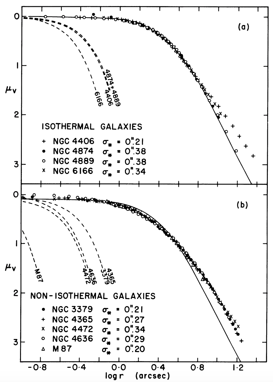
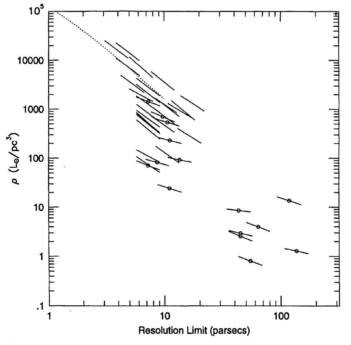
Figure 12.3: Core (isothermal) and power-law (non-isothermal) elliptical galaxies. Left: surface brightness profiles for the cores of selected elliptical galaxies (Kormendy 1985). Right: luminosity density at the innermost resolved point from the comprehensive study of Lauer et al. (1995). Galaxies with near-isothermal cores are marked with a dot in the right panel.

This figure shows galaxies that are well represented as isothermal cores (King profiles) and galaxies that deviate slightly, but significantly from the isothermal behavior. HST observations showed that even the isothermal galaxies do not reach a constant surface brightness at any resolved radius and keep increasing as close as 10 pc from the center (see the right panel of Figure 12.3); despite this behavior, the near-isothermal galaxies are referred to as cored galaxies. The near-isothermal galaxies have power-law slopes \(\gamma\) of their surface brightness \(I(R) \propto R^{-\gamma}\) that lie in the range \(0 \lesssim \gamma \lesssim 0.3\), while the power-law galaxies have \(\gamma \approx 1\). Which class an elliptical galaxy falls in correlates with their luminosity: more luminous ellipticals are near-isothermal (core) galaxies, while less luminous ellipticals display a \(\gamma \approx 1\) power-law (Kormendy 1985). The power-law behavior discussed here is that of the surface brightness, which is a projection of the 3D luminosity density. We can de-project it using the Abel inversion of Equation (6.17), which can be difficult. Roughly speaking, near-isothermal galaxies have inner luminosity density slopes \(\alpha\) in \(L(r) \propto r^{-\alpha}\) that are \(0 \lesssim \alpha \lesssim 1\) and thus shallow cusps, while the power-law galaxies with \(\gamma \approx 1\) have steeper cusps with \(1 \lesssim \alpha \lesssim 2\). To represent the surface-brightness profiles of the centers of ellipticals, an often-used form is the so-called “Nuker profile” (Lauer et al. 1995; Byun et al. 1996; named after the team that proposed it) \begin{equation} I(R) = 2^{(\beta-\gamma)/\alpha}\,I_b\,\left({R_b\over R}\right)^\gamma\,\left(1+\left[{R \over R_b}\right]^\alpha\right)^{(\gamma-\beta)/\alpha}\,. \end{equation} This profile is such that at \(R \ll R_b\) the surface brightness is approximately \(I(R) \propto R^{-\gamma}\), while at \(R \gg R_b\), approximately \(I(R) \propto R^{-\beta}\); the parameter \(\alpha\) sets how sharply the profile transitions between these two behaviors at \(R \approx R_b\). This profile is similar to the two-power density profiles of Chapter 2.4.6, but note that the Nuker profile is for the surface-brightness. To obtain the three-dimensional density, one has to de-project the Nuker profile using the Abel inversion of Equation (6.17). This, however, cannot be done using elementary or simple special functions (again, instead, requiring the dreaded “Fox H function” ; Baes 2020) and using the Nuker profile for dynamical studies is therefore difficult. Approximating the surface-brightness with a suitable two-power density profile of Chapter 2.4.6 is therefore again a useful strategy for dynamical studies of the inner regions of elliptical galaxies.

The isophotes of elliptical galaxies are, as their name implies, generally elliptical. Contours of the projected shape of elliptical galaxies are typically well-represented as a set of eccentric ellipses with axis ratio \(b/a\) and ellipticity \(\varepsilon = 1-b/a\). For example, in the Hubble classification scheme (Hubble 1926), elliptical galaxies are arranged by ellipticity starting from \(\varepsilon=0\) to \(\varepsilon = 0.7\), which is about as elliptical as any observed elliptical galaxy ever gets; the Hubble classification explicitly uses this projected ellipticity as part of its name, as \(\mathrm{E}[10\varepsilon]\), where \([\cdot]\) rounds to the nearest integer (e.g., E2 indicates a galaxy with ellipticity 0.2).

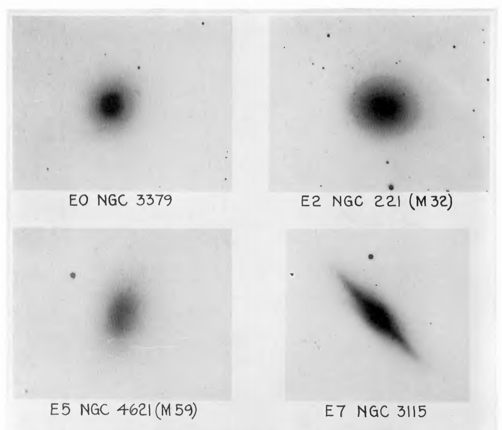
Figure 12.4: Elliptical galaxies with different ellipticities (adapted from Hubble 1926).

Some examples are shown in Hubble (1926)’s original paper, reproduced here in Figure 12.4.

For any external elliptical galaxy, we can only measure its projected shape on the sky and it is therefore not immediately clear that elliptical galaxies cannot be represented as axisymmetric distributions seen from a random viewpoint. The simplest interpretation of the projected elliptical shape was therefore that the intrinsic shape of elliptical galaxies was axisymmetric with an intrinsic axis ratio \(q\) that satisfies \(q < 1-\varepsilon\). Axisymmetric models were therefore the starting point for interpreting observations of elliptical galaxies (e.g., Wilson 1975). However, various lines of evidence argue against axisymmetric models for elliptical galaxies. Photometrically, the distribution of observed shapes is inconsistent with that resulting from projecting an intrinsically axisymmetric distribution with a range of axis ratios (Ryden 1996). Additionally, the projected major axis of many elliptical galaxies twists on the sky (known as isophotal twists; King 1978), which could be due to an actual twist of the major axis of axisymmetric shells or, more naturally, result from a smooth change in the axis ratios of a triaxial model (Binney 1978a); in both cases, the overall mass distribution is non-axisymmetric. Kinematically, flattened axisymmetric models are expected to rotate significantly (Binney 1978b; see Chapter 14.2), while early observations indicated only mild rotation in many ellipticals (Bertola & Capaccioli 1975; Illingworth 1977). Triaxial bodies typically contain stable orbits that circulate around the major axis (in addition to orbits that circulate around the minor axis, which also exist in axisymmetric mass distributions), which gives rise to observed rotation along the projected minor-axis (Contopoulos 1956; Binney 1985); small amounts of such minor-axis rotation have been observed (Franx et al. 1991). All of these observations indicate that there is at least some triaxiality in the mass distributions of elliptical galaxies. Modern observational campaigns that measure two-dimensional kinematics of many elliptical galaxies separate ellipticals into two classes based on their mean rotation: slow rotators and fast rotators (e.g., Cappellari 2016). The lower-mass fast rotators have kinematics that aligns with their observed photometry; this lack of minor-axis rotation indicates that they are close to axisymmetric and their orbital structure is therefore not so different from that of disks. Slow rotators, which are typically more massive, are likely mildly triaxial (e.g., Weijmans et al. 2014).

One final aspect of the shape of elliptical galaxies that is important is that their isophotes systematically deviate from being pure ellipses in a manner that is correlated with other galaxy properties. Deviations from pure elliptical isophotes are typically measured by first finding the best-fit pure ellipse for a given isophote and then expanding the radial differences \(\Delta r\) between the observed isophote and the ellipse model as a function of azimuthal angle \(\theta\), in coordinates where the ellipse’s major axis is at \(y=0\), as (e.g., Bender & Moellenhoff 1987) \begin{equation} \Delta r(\theta) = a_0 + \sum^N_{n=1}\,a_n\cos (n\theta) + b_n \sin (n\theta)\,. \end{equation} Because the deviations are measured with respect to the best-fitting ellipse, the coefficients \(a_0\), \(a_1\), \(b_1\), \(a_2\), and \(b_2\) are all \(\approx 0\) and the higher-order coefficients then measure deviations from ellipticity. Among the coefficients with \(n \leq 5\), the \(a_4\) coefficient is the only one that describes deviations that are symmetric with respect to both the major and minor axis of the ellipse, which is generally what is observed. Therefore, the \(a_4\) coefficient is typically the only non-zero \(n\leq5\) coefficient. Its importance is that it describes deviations from ellipticity that are either disky, for \(a_4 > 0\), or boxy, for \(a_4 < 0\). The strength of the diskyness or boxyness is determined by the ratio \(a_4/a\) of the \(a_4\) coefficient to the semi-major axis of the ellipse \(a\). Figure 12.5 displays two archetypal examples from the original disky-vs-boxy analysis of Bender et al. (1988) as well as an exaggerated illustration of the effect of disky or boxy \(a_4\) coefficients on an isophote’s shape.

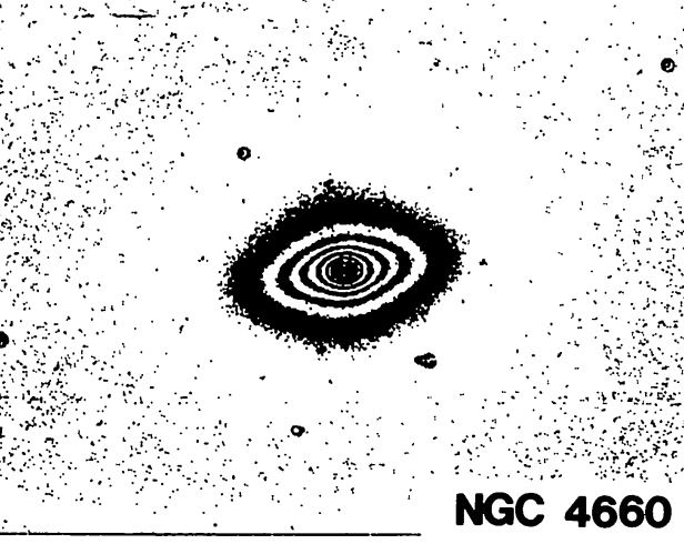
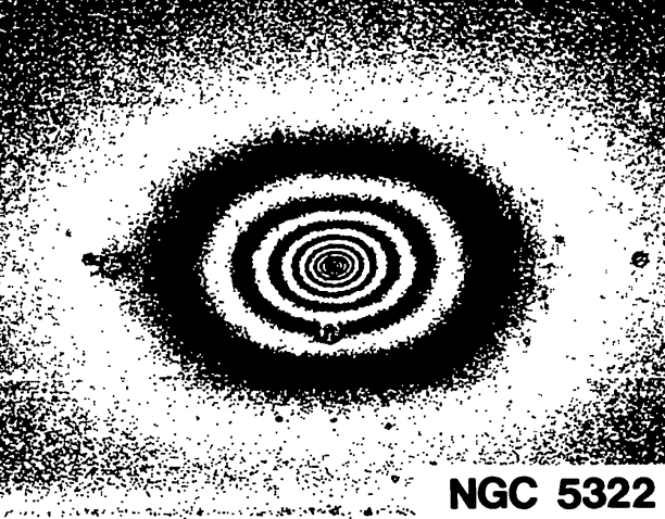
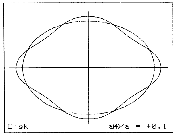
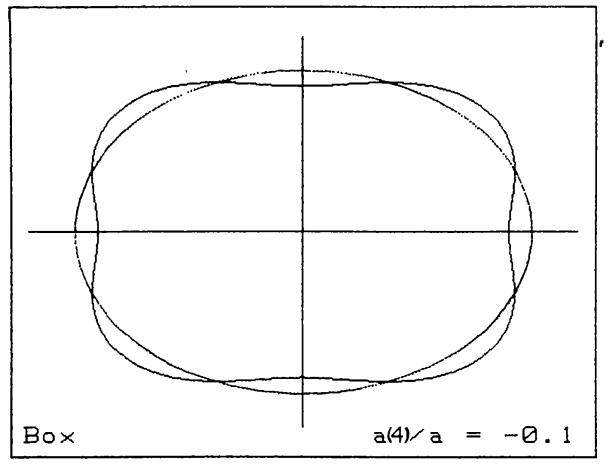
Figure 12.5: Disky and boxy isophotes in elliptical galaxies (Bender et al. 1988).

We see that even a small disky \(a_4\) coefficient (\(a_4/a \approx 0.03\) for NGC 4660) makes a galaxy’s isophotes resemble those of a disk galaxy (see, for example, the isophotes of NGC 4244 in Figure 1.9). A small boxy \(a_4\) coefficient (\(a_4/a\approx -0.01\) for NGC 5322) makes a galaxy almost look like a rectangle with rounded corners. The importance of disky vs. boxy isophotes is that this property is correlated with other galaxy properties and, in particular, the slow rotators discussed above generally have boxy isophotes, while the fast rotators have disky isophotes. We will discuss the relations between the different observational properties of elliptical galaxies discussed in this section in more detail in Chapter 16, in particular in Section 16.4.

The second class of mass distributions that we study in this part are dark-matter halos. Observational constraints of the shape of dark-matter halos are scant, but they have been studied in detail in numerical simulations. Dissipationless simulations—also known as dark-matter only simulations—create galactic dark-matter halos that are strongly triaxial and highly flattened (e.g., Frenk et al. 1988; Dubinski & Carlberg 1991; Jing & Suto 2002). Moreover, compared to elliptical galaxies, dark matter halos are much more flattened. Labeling the relative lengths of the major, intermediate, and minor axis as \(a \geq b \geq c\), dissipationless dark-matter halos have typical values of \(b/a \approx 0.7\) and \(c/a \approx 0.5\). Some of these results are illustrated in Figure 12.6.

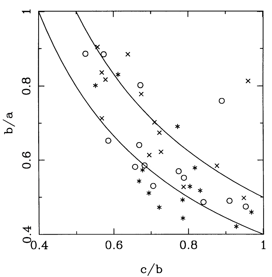
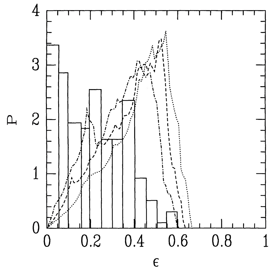
Figure 12.6: Shape of simulated dark-matter halos from Dubinski & Carlberg 1991. Left: axis ratios of simulated dark matter halos at different radii (25 kpc [asterisks], 50 kpc [circles], and 100 kpc [crosses]). Right: distribution of observed ellipticities in the sample of elliptical galaxies of Binney & de Vaucouleurs (1981) compared the projected ellipticities of simulated dark matter halos.

The shape of a triaxial density is also often summarized using the triaxiality parameter \(T\) defined as \begin{equation}\label{eq-triaxialgrav-triaxility-parameter} T = {a^2-b^2 \over a^2-c^2} = {1-(b/a)^2 \over 1-(c/a)^2}\,. \end{equation} From the definition of \(T\), it is clear that oblate (\(a = b > c\)) and prolate (\(a > b = c\)) distributions have \(T=0\) and \(T=1\), respectively. Mass distributions with \(T = 0.5\) are then maximally-triaxial. For the canonical \(b/a \approx 0.7\), \(c/a \approx 0.5\) mentioned above, we get \(T \approx 0.7\). Generally, dissipationless dark-matter halos are more prolate than oblate (\(T > 0.5\)). The shape parameters \(b/a\), \(c/a\), and \(T\) depend on radius, with a generally more axisymmetric, prolate shape within a tenth of a virial radius (\(T \approx 1\)) deforming to a strongly triaxial shape near the virial radius (\(T \approx 0.5\); e.g., Chua et al. 2019). We discuss the reason for the triaxial shape in dissipationless simulations further in Chapter 17.3.4 and the effect of the growth of a central galaxy on the shape of the dark-matter halo in Chapter 13.4.3.

Numerical studies of the orbital structure of such triaxial distributions show that they are stable over the age of the Universe (e.g., Aarseth & Binney 1978; Schwarzschild 1979; van Albada 1982). The dissipational growth of a baryonic component in galaxies has the effect of making the inner parts of dark-matter halos axisymmetric (e.g., Dubinski 1994), but the outer regions of halos remain triaxial. Aside from affecting the dynamics of stars, clusters, satellites, and everything else embedded within the dark matter halos that host galaxies, the shape of dark matter halos also holds valuable clues about the nature of dark matter, because, for example, strong self-interactions between dark matter particles would tend to sphericalize it (e.g., Spergel & Steinhardt 2000).

Therefore, to fully understand the structure of elliptical galaxies and dark matter halos, we need to investigate the gravitational potential, orbits, and equilibrium states of triaxial mass distributions. We will start by discussing simple models for flattened-axisymmetric and triaxial distributions, which have shapes and orientations that are constant with radius. However, it is clear from the discussion above that realistic galaxies and dark-matter halos have shapes that change with radius: Elliptical galaxies with isophote twists either require the orientation or the shape to change with radius (and perhaps both!); dark-matter halos are likely axisymmetric and only mildly flattened in their inner parts due to the growth of the baryonic component, while they are expected to be strongly triaxial in their outer parts. To handle this complexity, we will present several general, yet practical, approaches to solving the Poisson equation for any mass distribution, including the complex, evolving mass distributions encountered during galaxy assembly studied in N-body modeling.

← Previous section Next section →