
1.2. A brief tour of galaxy observations
To set the stage for the material covered in this book, we start with a high-level overview of the various components that make up galaxies. The objective here is not to provide a detailed and exhaustive overview of galaxy phenomenology (that will be done in later chapters!), but merely to briefly discuss the size, shape, and contribution to the overall mass budget of different galactic components.
We will focus our overview on large disk galaxies. Large disk galaxies are one of the most important type of galaxies for various reasons: approximately half of all galaxies in the local Universe are disk galaxies and such galaxies appear to be most efficient at converting gas into stars. Therefore, most stars in the local Universe live in the disks of large disk galaxies. We also live close to the mid-plane of a large disk galaxy, the Milky Way. This provides us with a detailed, close-up view of the structure of such a galaxy. In the Milky Way, we can observe stars from the most luminous giants to the lowest mass M dwarfs, from the center of the Galaxy to the outskirts of the spherical stellar halo surrounding the disk, and we can study gas in its various atomic and molecular phases. Because galactic disks are “dynamically cold”, meaning that the ratio of their velocity dispersion to the typical velocity of a star is small, they are also prone to instabilities that give rise to bars, spiral structure, etc., which are phenomena that we will discuss in later chapters.
Figure 1.6 shows a typical disk galaxy, NGC 4565, seen edge-on.
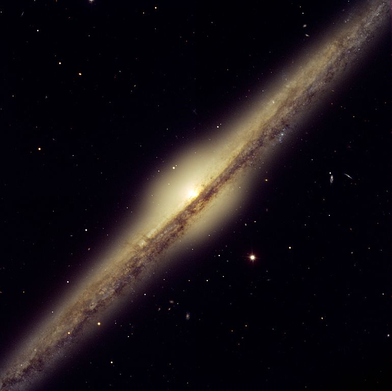
Figure 1.6: NGC 4565, an edge-on disk galaxy (ESO).
NGC 4565 displays all of the components of a typical disk galaxy. Its structure is dominated by a disk consisting of stars and gas, with a protrusion of stars near the center that is called the bulge. The gas itself cannot be seen in this picture, but its presence can be inferred because gas is traced by dust grains, which redden passing starlight and cause the reddish band close to the disk’s mid-plane. NGC 4565 does have a stellar halo (Harmsen et al. 2017), but it is too faint to be seen in this picture. Also not seen in this picture (and never seen directly—whatever that means—in any picture of any galaxy) is the spheroidal distribution of dark matter that surrounds the disk and extends to very large distances from the center.
Figure 1.7 provides a schematic overview of a disk galaxy, the Milky Way in particular (but except for the Sun’s position, this structure applies to all disk galaxies).
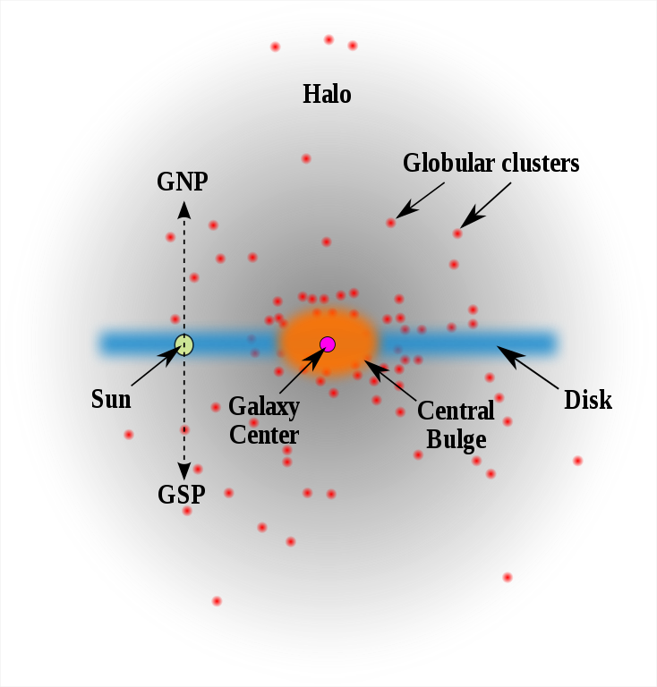
Figure 1.7: A schematic overview of the Milky Way (RJHall at English Wikipedia).
This illustration shows the disk edge-on and displays the system of globular clusters that surrounds each galaxy in addition to the components that we already discussed. The Galactic center is also separately emphasized. We have known for about two decades that the centers of galaxies host supermassive black holes (see Chapter 16), which can be active and surrounded by an accretion disk (such accretion disks are a topic that we will not cover in this book) or inactive and often surrounded by a dense nuclear star cluster.
1.2.1. The distribution of stars in galaxies
One of the most basic observations about the disks of galaxies is that they are exponential. That is, their light profiles \(I(R)\) follow an exponential decline with radius \(I(R) = I_0\,\exp\left(-R/h_R\right)\). This had been known in the mid-1900s, but was most famously discussed by Freeman (1970) “On the disks of spiral and S0 galaxies” (oh, to be able to write a paper with a title like that!). Figure 1.8 is the first figure in Freeman’s paper, which shows the surface brightness as a function of radius along the major axis in the blue B band.
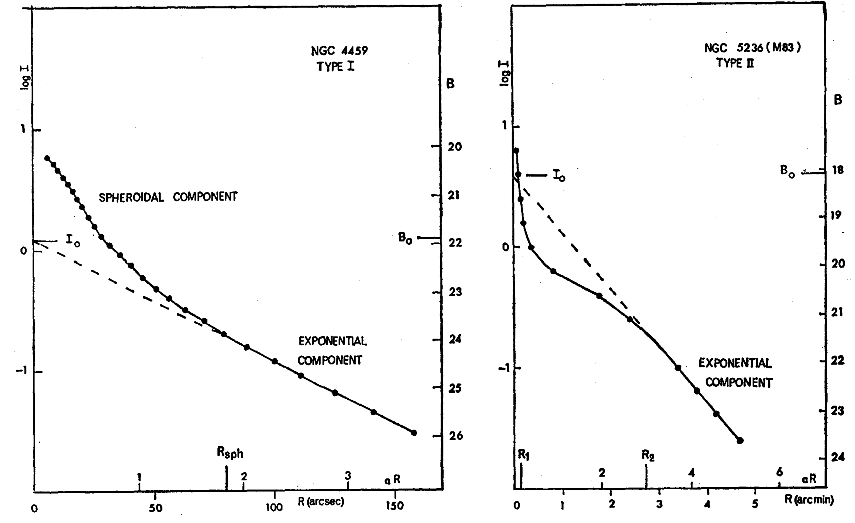
Figure 1.8: Galaxy disks have exponential profiles (Freeman 1970).
Because surface brightness is given on the y axis as a logarithmic quantity measured in magnitudes, the linear decline implies an exponential decline of the light profile. Both of the shown galaxies only follow the exponential law over a restricted radial range. Near the center they rise precipitously, due to the presence of the bulge (the “spheroidal component” above); the galaxy on the right also has a flattened part of the light profile near the center, which is not uncommon.
The second most important dimension of a disk is its vertical dimension. Vertical for the moment means perpendicular to the two-dimensional plane of the disk, the direction along which the disk is narrowest. Along the vertical direction, the density also falls off quickly in a roughly symmetric manner; the peak of the vertical density occurs at the mid-plane, the zero-point of the vertical coordinate. Like for the radial profile, we look at the vertical profile of the surface brightness to get a sense for what the vertical mass distribution is. Figure 1.9 shows a typical result.
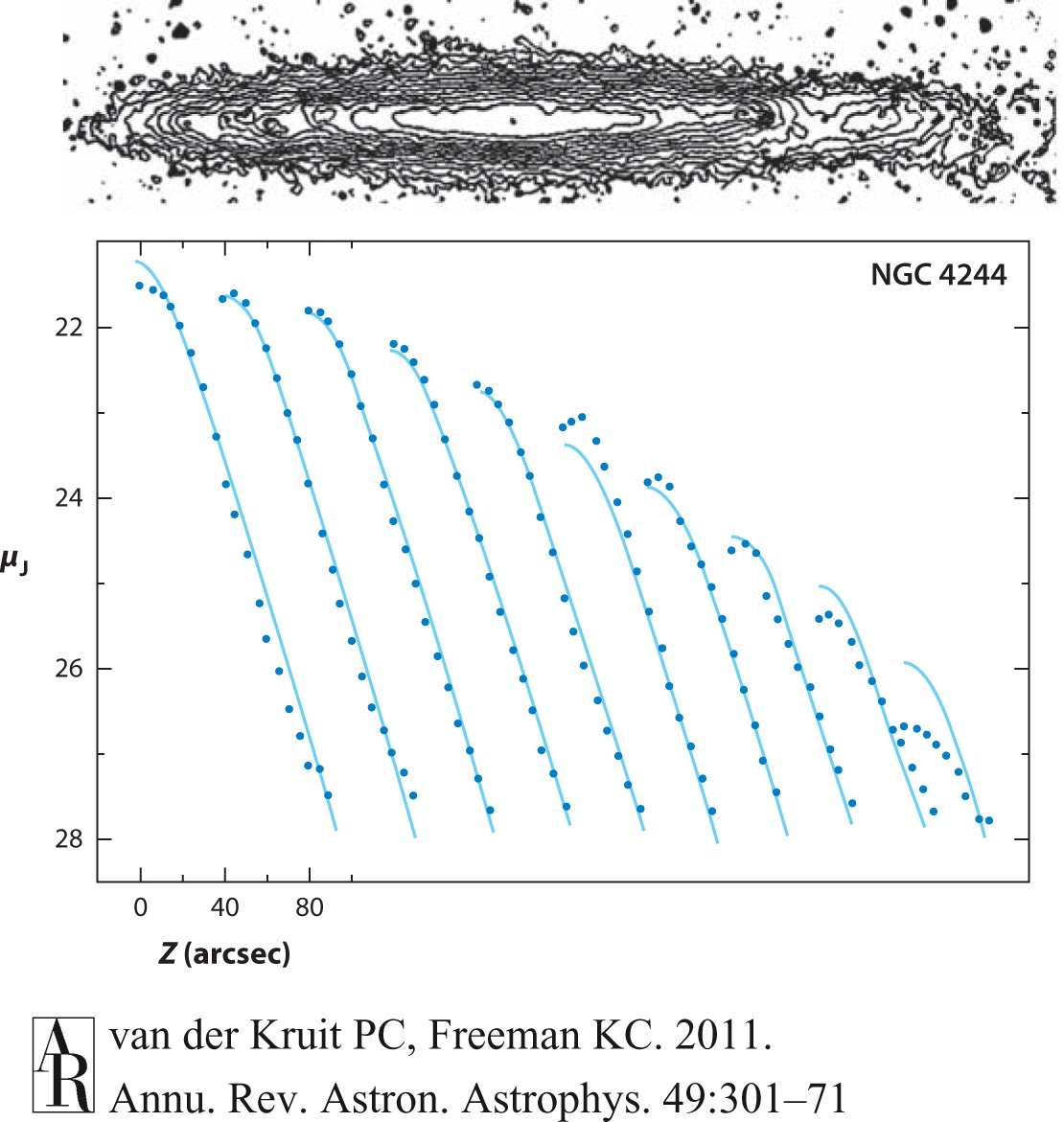
Figure 1.9: NGC 4244: top: a pure-disk galaxy seen edge-on; bottom: vertical surface-brightness profiles at a range of distances from the center; profiles are displaced along the X axis to avoid overlap (van der Kruit & Freeman 2011).
This figure shows vertical surface-brightness profiles for NGC 4244 at different distances from its center. Again we see a linear decline at large distances, which implies an exponential fall-off (because the surface-brightness in this figure is again a logarithmic quantity). Near the mid-plane the profile flattens and becomes close to constant. The fit that is shown is a \(\mathrm{sech}^2\) profile, a hyperbolic secant squared, which is the equilibrium solution of a self-gravitating isothermal disk as we will see in Chapter 10.4. As we discussed above and will discuss below in more detail, disks contain gas and stars of various ages with different vertical distributions and the simple isothermal—having the same amount of random motion at each vertical height—can therefore not be entirely correct. The \(\mathrm{sech}^2\) profile should therefore not be taken too seriously, but is simply a physically-motivated profile that does a good job of fitting the observations.
The ratio between the scale length \(h_R\) of the radial decline and the scale height \(h_z\) of the vertical decline is a measure of the thickness of the disk. A typical value is \(h_R / h_z \approx 10\), meaning that disks are quite thin.
Whether we use number counts or surface brightness, to translate these observed profiles to mass profiles we have to assume stellar-population models for how mass is traced by light. This is done by applying a mass-to-light ratio \(M/L\) that converts the amount of light observed to an amount of (stellar) mass and is usually silently expressed in solar units (the Sun’s mass over the Sun’s luminosity). The stellar mass-to-light ratio is typically assumed to be constant through the galaxy and is \(M/L \approx 3\), but it depends on the passband in which the luminosity is measured. The total mass-to-light ratio in galaxies is much larger and depends on position, because in addition to stars it includes the dark matter, which adds mass, but does not contribute to the luminosity; the total \(M/L\) also includes gas, which in broad optical and near-infrared passbands similarly does not contribute to the luminosity, while adding mass (but generally much less mass than either stars or dark matter; see below). The total mass-to-light ratio depends on position because the fraction of total mass that is dark matter and gas strongly depends on position.
While the radial and vertical profiles of the disk are (close to) exponential, the central bulge is not. Bulges typically have profiles similar to elliptical galaxies, which are modeled as Sérsic profiles: \(\mu(R) = \mu_0 - b_n R ^{1/n}\), where \(\mu\) is the surface brightness, \(\mu_0\) is the central surface brightness, \(n\) is the Sérsic index, and \(b_n\) can be computed from the value of \(n\). The case of \(n=4\) is the classic de Vaucouleurs profile, which represents the surface brightness profiles of large elliptical galaxies well. Setting \(n=1\), we have an exponential profile.
As an example, Figure 1.10 displays the surface-brightness profile of M31, the closest large disk galaxy outside of the Milky Way.
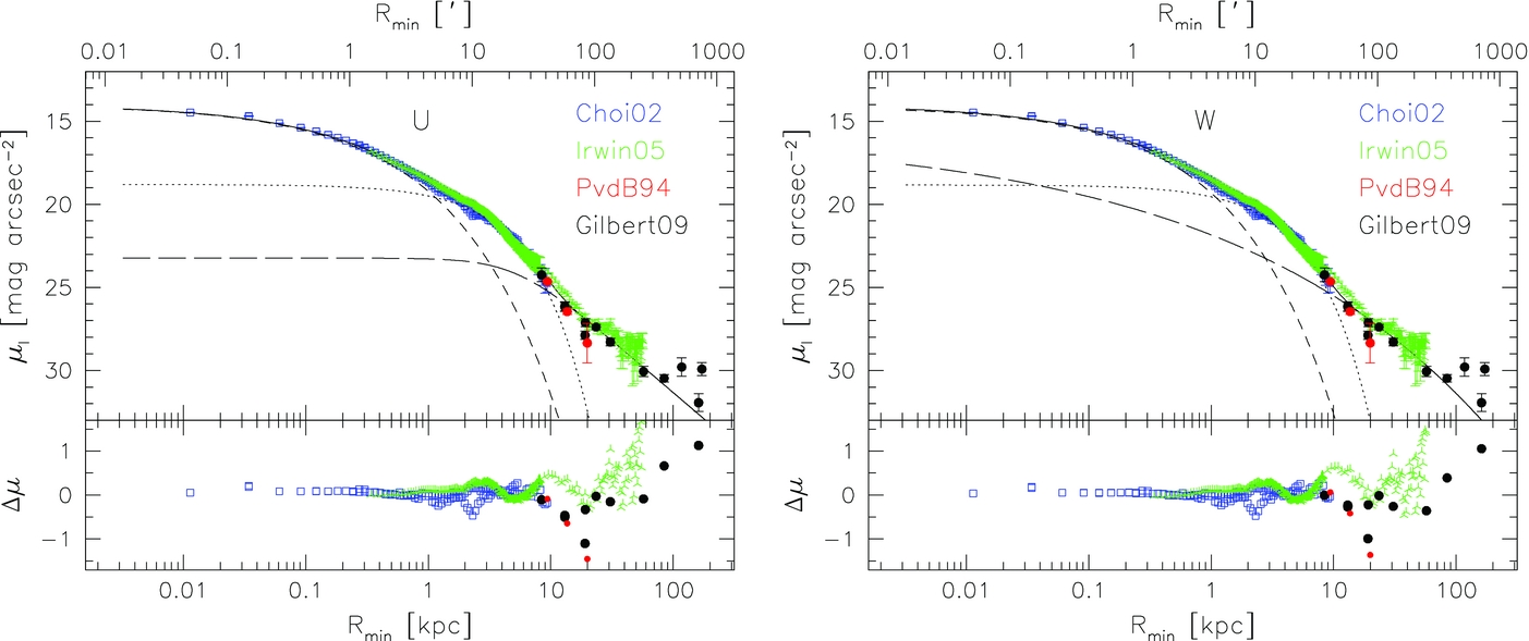
Figure 1.10: Surface-brightness profile of M31 along with a fit with a Sérsic bulge (dashed), exponential disk (dotted) and halo (long dashed) with the combined fit profile as the full curve; halo model is a power-law on the left and Sérsic on the right (Courteau et al. 2011).
M31’s bulge component is a dashed line in fits to this profile with a Sérsic bulge, exponential disk, and a stellar halo (with two different radial profiles in the two panels). The bulge has a Sérsic index of about 2.2 and dominates within 1 kpc, the very central region of the galaxy. The disk, given by the dotted line, starts to dominate the light outside of 1 kpc and does so out to 10 kpc. The stellar halo dominates the light outside of the disk region.
Given how prominent the stellar halo is outside of the disk region, let’s take a closer look at this component. Figure 1.11 shows deep observations of some external disk galaxies. These observations are deep enough to reveal the low surface-brightness envelope surrounding these disks (the actual disks are painted in from shallower observations).
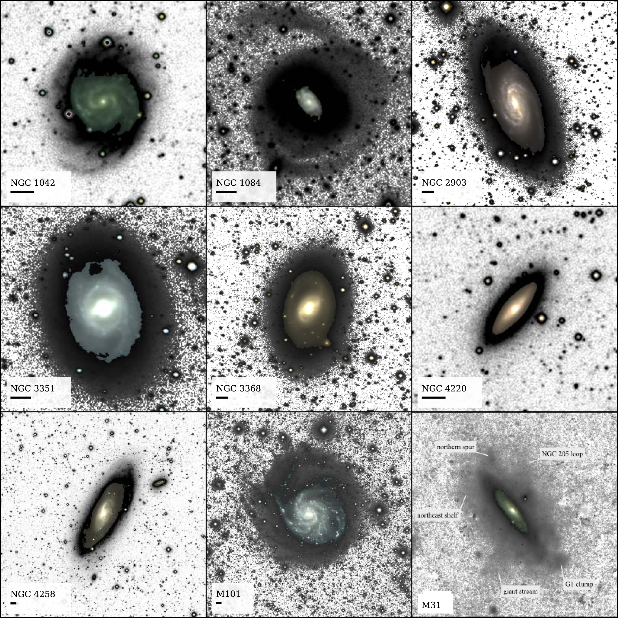
Figure 1.11: Stellar halos (Merritt et al. 2016).
When fitting the radial surface-brightness profile of these galaxies with an exponential-disk plus a bulge, many of these galaxies have excess light at large radii (\(> 20\,\mathrm{kpc}\)) beyond the exponential disk. This light extends in a spheroidal manner, not a disk, and follows an approximate power-law profile. There is great diversity in the profiles of the stellar halos in galaxies. This is because the stellar halo is believed to form primarily from mergers (accreted material from merging satellite galaxies, or material from the main galaxy disturbed by a merger).
While the stellar halo takes up a large volume, its total stellar mass is much smaller than that of the other main galactic components. The stellar halo typically only accounts for a few percent of the stellar mass of a galaxy and much less than that of the total mass. There is no part of a galaxy where the stellar halo dominates the density, because it is always overwhelmed by either the bulge, disk, dark-matter halo, or the gaseous component.
1.2.2. The distribution of gas in galaxies
All baryonic matter was once in gaseous form, but in large, present-day disk galaxies only about 10% of the baryonic mass is present as cold/warm gas in the interstellar medium. Gas is present in galaxies in different phases and in both atomic and molecular form. Making a precise census of all of the gas in galaxies, in particular the amount of hot halo gas, is difficult.
Stars form from cold molecular gas. Cold gas is contained in a disk component much like the stellar disk component that we discussed above. Most of the gas is atomic hydrogen, or HI. Figure 1.12 shows the cold-gas content (HI in particular) as a function of stellar mass for a sample of galaxies in the local Universe.
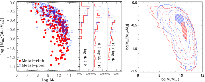
Figure 1.12: The gas content of galaxies (Zhang et al. 2009). Left panel: HI gas mass fraction vs. stellar mass for metal-rich (red) and metal-poor (blue) galaxies, for galaxies with direct HI observations. Right panel: HI mass fraction vs. stellar mass for star-forming galaxies with indirect HI measurements.
The Milky Way’s stellar mass is about \(6 \times 10^{10}\,M_\odot\) or \(\log (M_*/M_\odot) \approx 10.8\) (Bovy & Rix 2013); gas makes up about 10% of the baryonic disk mass in the Milky Way. Figure 1.12 shows that the gas fraction rises as one goes to lower mass galaxies and the dynamics of gas and its interaction with stars is thus much more important in lower mass galaxies than it is in the Milky Way.
In the Milky Way, we can make a reasonably complete census of the interstellar medium near the Sun. The main components are: atomic hydrogen (HI), ionized hydrogen (HII), and molecular hydrogen (\(H_2\)) contributing \(\approx 1.01\,\mathrm{cm}^{-3}\), \(\approx 0.015\,\mathrm{cm}^{-3}\), and \(\approx 0.15\,\mathrm{cm}^{-3}\), respectively in the mid-plane (McKee et al. 2015). The atomic hydrogen comes in cold and warm phases that constitute \(\approx 80\%\) and \(\approx 20\%\) of the local HI density. Converting these number densities in the mid-plane to a mass density, we find that the mid-plane gas density is about \(0.041\,M_\odot\,\mathrm{pc}^{-3}\), approximately the same as that in stars (\(\approx 0.040\,M_\odot\,\mathrm{pc}^{-3}\); Bovy 2017b). The molecular gas layer has an exponential scale height that is approximately \(h_z = 100\,\mathrm{pc}\), the cold component of HI has about the same thickness, the warm HI has \(h_z \approx 300\,\mathrm{pc}\), while the ionized gas is contained in a much thicker layer. The total local gas surface density is \(\approx 14\,M_\odot\,\mathrm{pc}^{-2}\) with HI contributing \(\approx 11\,M_\odot\,\mathrm{pc}^{-2}\), HII \(\approx 2\,M_\odot\,\mathrm{pc}^{-2}\), and \(H_2\) adding \(\approx 1\,M_\odot\,\mathrm{pc}^{-2}\).
The radial distribution of these gas components is much less certain. The radial surface density of HI is shown in the left panel of Figure 1.13.
|
|

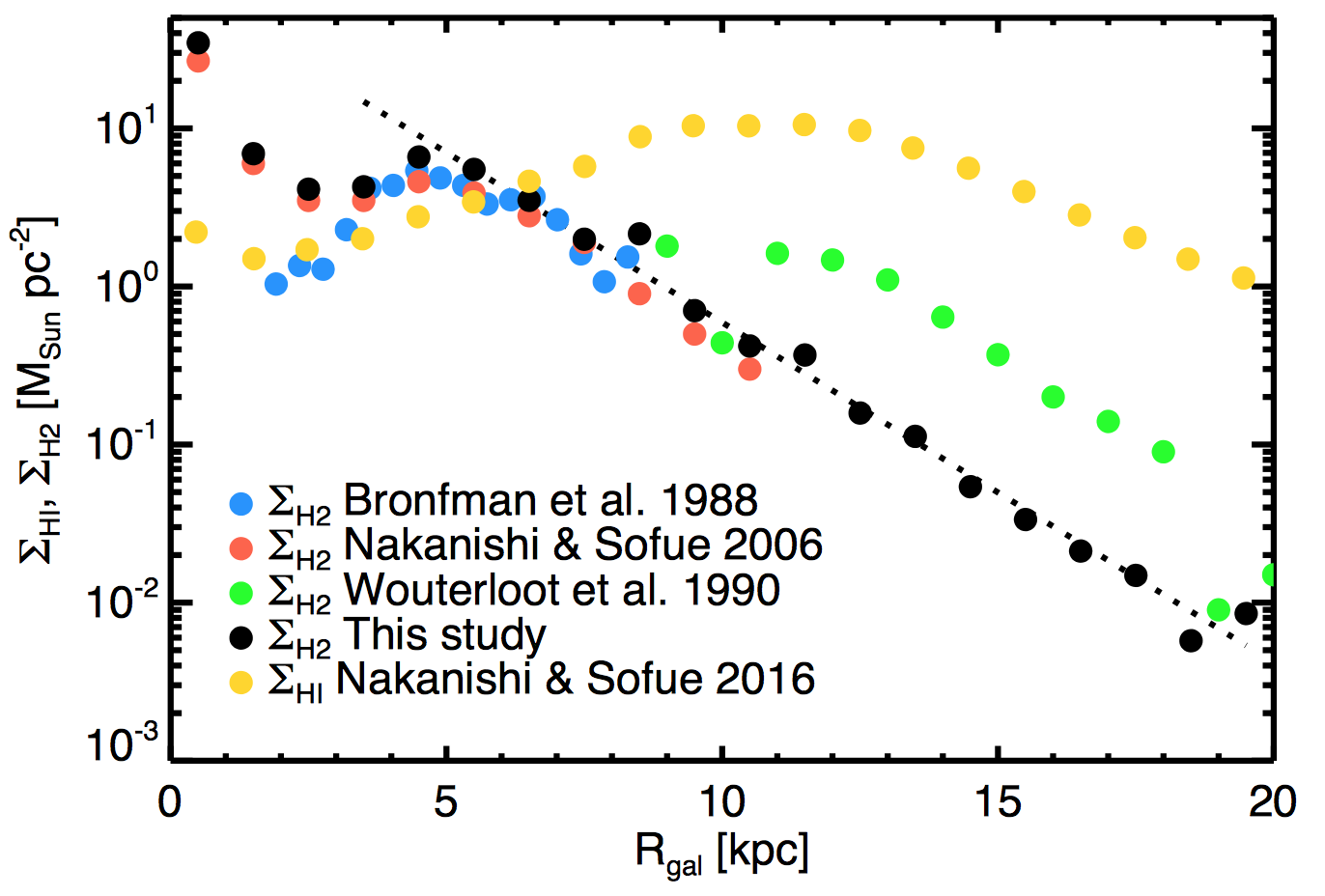
Figure 1.13: The surface density of neutral hydrogen (Kalberla & Kerp 2009; left panel) and of molecular hydrogen (Miville-Deschênes et al. 2017; right panel) in the Milky Way.
Thus, the density of HI is almost constant within 10 kpc or at most displays a shallow decline; outside of 10 kpc it falls off exponentially. But note that there are significant asymmetries between different parts of the distribution.
A smaller fraction of the ISM is contained in molecular gas (about 10% near the Sun). The radial profile of the molecular gas is similar to that of the HI: it is approximately constant in the inner Galaxy and drops off exponentially at larger radii, as shown in the right panel of Figure 1.13. But the molecular gas has a shorter scale length than the HI, so very little of it is found outside of 15 kpc. Almost all of the molecular gas is contained in molecular clouds.
The figure above was made from a recent molecular-cloud catalog. We load this catalog from Miville-Deschênes et al. (2017) in the following interactive figure:
This figure shows the molecular clouds in the disk plane of the Milky Way as seen from above, with the Sun at \((X,Y) = (8,0)\) kpc. The area of the points is proportional to the total mass of each cloud (with a simple linear scaling) and the points are color-coded by their velocity with respect to the Sun. You can zoom in and out to get a closer look at the distribution. It is clear that most of the large clouds are located closer to the center than the Sun is. The velocity pattern is also clearly not random! What creates this pattern of velocities? After reading Chapter 8 you should be able to answer this question. The answer isn’t as obvious as you might think!
1.2.3. The distribution of mass in galaxies
Now that we have a good sense of the stellar and gas distribution in a typical disk galaxy, let’s take a look at the largest contributor to the galactic mass distribution: the dark-matter halo. Dark matter is a largely unknown constituent of the Universe, likely a new particle, that overall is about 5 times more abundant (e.g., Planck Collaboration et al. 2016) than ordinary matter (sometimes called “baryonic matter” although this misses the ordinary, fermionic matter that is, however, negligible in mass compared to its baryonic counterpart). In galaxies such as the Milky Way there is more than ten times more dark matter than ordinary matter, with the remaining baryonic matter likely in warm and hot phases in the interstellar and intergalactic medium (e.g., Shull et al. 2012). We know about the presence of dark matter solely through its gravitational influence and this book will cover how we have learned and are continuing to investigate the distribution of dark matter in galaxies.
To get a sense of the distribution of dark matter, we will plot the density and enclosed mass of different components of the Milky Way. We use the mass model for the Milky Way from McMillan (2017). This model has a bulge, disk, and dark-matter halo potential (ignoring the contributions from the stellar halo and including those from the gas together with the stellar disk). In the top panel of Figure 1.14, we look at the density of the different components in the mid-plane of the Milky Way (at \(z = 0\)) as well as the total density.
[10]:
from functools import reduce
from galpy import potential
from galpy.potential.mwpotentials import McMillan17
from galpy.util import plot as galpy_plot
from matplotlib.ticker import FuncFormatter
from astropy.visualization import quantity_support
figure(figsize=(8,8))
rs= 10.**(numpy.linspace(-1.,2.5,101))*u.kpc
subplot(2,1,1)
# Bulge
line_bulge= galpy_plot.plot(\
                rs,
                McMillan17[2].dens(rs,0.0*u.kpc),
                lw=2.,label=r'$\mathrm{Bulge}$',loglog=True,
                ylabel=r'$\rho(r,z=0)\,(M_\odot\,\mathrm{pc}^{-3})$',
                xrange=[0.1,400.],yrange=[10.**-5.7,70.],gcf=True)
# Disk
line_disk= loglog(rs,
                  McMillan17[0].dens(rs,0.0*u.kpc),
                  lw=2.,label=r'$\mathrm{Disk}$')
# DM halo
line_dm= loglog(rs,
                McMillan17[1].dens(rs,0.0*u.kpc),
                lw=2.,label=r'$\mathrm{Dark\ matter\ halo}$')
# Full
alldens= [reduce(lambda x,y: x+y,[pot.dens(r,0.0*u.kpc)
          for pot in McMillan17]) for r in rs]
alldens= numpy.array([d.to(u.solMass/u.pc**3).value for d in alldens])\
            *u.solMass/u.pc**3
line_full= loglog(rs,alldens,
                  color='k',lw=2.,label=r'$\mathrm{Combined}$')
legend(handles=[line_bulge[0],line_disk[0],line_dm[0],line_full[0]],
       fontsize=18.,loc='upper right',frameon=False)
gca().xaxis.set_major_formatter(FuncFormatter(
                lambda y,pos: (r'${{:.{:1d}f}}$'.format(int(\
                    numpy.maximum(-numpy.log10(y),0)))).format(y)))
subplot(2,1,2)
rs= 10.**(numpy.linspace(-1.,2.5,101))*u.kpc
# Bulge
bulge_mass_enc= numpy.zeros(len(rs))*u.solMass-1.*u.solMass
bulge_mass_enc[rs < 10.*u.kpc]= \
    numpy.array([McMillan17[2].mass(r).to(u.solMass).value
                 for r in rs if r < 10.*u.kpc])*u.solMass
bulge_mass_enc[rs >= 10.*u.kpc]= numpy.amax(bulge_mass_enc)
line_bulge= galpy_plot.plot(rs,bulge_mass_enc,loglog=True,
                            lw=2.,label=r'$\mathrm{Bulge}$',
                            xlabel=r'$r\,(\mathrm{kpc})$',
                            ylabel=r'$M(<r)\,(M_\odot)$',
                            xrange=[0.1,400.],
                            yrange=[10.**7.5,10.**12.5],
                            gcf=True)
# Disk, only compute out to where density is appreciable
disk_mass_enc= numpy.zeros(len(rs))*u.solMass-1.*u.solMass
disk_mass_enc[rs < 50.*u.kpc]= \
    numpy.array([McMillan17[0].mass(r).to(u.solMass).value
                 for r in rs if r < 50.*u.kpc])*u.solMass
disk_mass_enc[rs >= 50.*u.kpc]= numpy.amax(disk_mass_enc)
line_disk= loglog(rs,disk_mass_enc,lw=2.,label=r'$\mathrm{Disk}$')
# DM halo
halo_mass_enc= numpy.array([McMillan17[1].mass(r).to(u.solMass).value
                            for r in rs])*u.solMass
line_dm= loglog(rs,halo_mass_enc,lw=2.,label=r'$\mathrm{Dark\ matter\ halo}$')
# Full
full_mass_enc= bulge_mass_enc+disk_mass_enc+halo_mass_enc
line_full= loglog(rs,full_mass_enc,
                  color='k',lw=2.,label=r'$\mathrm{Combined}$')
legend(handles=[line_bulge[0],line_disk[0],line_dm[0],line_full[0]],
       fontsize=18.,loc='upper left',frameon=False)
gca().xaxis.set_major_formatter(FuncFormatter(
                lambda y,pos: (r'${{:.{:1d}f}}$'.format(int(\
                    numpy.maximum(-numpy.log10(y),0)))).format(y)))
tight_layout(h_pad=0.5);

Figure 1.14: The mass profile of the Milky Way.
Much like in M31 above, the bulge component dominates the density within 1 kpc, but becomes less important after that. The stellar disk dominates the density between 1 kpc and about 30 kpc, after which the dark-matter halo dominates.
The total density near the Sun (at \(\approx 8\,\mathrm{kpc}\) from the center) is about \(0.1\,M_\odot\,\mathrm{pc}^{-3}\), with only about 1/10th of that contributed by dark matter. The bottom panel of Figure 1.14 shows the total mass enclosed within a given radius for the different components and for the total mass. The total mass in the bulge+disk is approximately equal to the total mass in the dark-matter halo within 10 kpc from the center. Outside of this, the dark-matter halo dominates the mass and at the edge of the Milky Way, around 250 kpc from the center, there is more than ten times as much dark matter as there is ordinary matter. We will have much more to say about the distribution of dark matter in later chapters.

 .
. .
. .
.