
18.5. Star formation in galaxies
So far in this chapter, we have discussed the luminosity, stellar mass, color, spectra, and morphology of galaxies and how they relate to the dynamical properties of the halo that they inhabit—dark matter mass, circular velocity, and velocity dispersion. The stellar luminosities, colors, and optical/near-infrared spectra that we observe are the result of star formation, the complex process of turning gas into stars. To finish our largely-observational overview of the galaxy population, we discuss the overall properties of star formation in galaxies and the Universe as a whole here.
As we saw in Section 18.3 above, one of the most important observational facts about the local galaxy population (which persists at least up to \(z\approx 3\)) is the bimodal color distribution of large galaxies. Plots of the galaxy population in color versus either absolute magnitude or stellar mass such as in Figure 18.20 show the existence of a tight red sequence and a more diffuse blue cloud. Correlating these with the morphological properties of galaxies demonstrates that the red sequence largely corresponds to the classical elliptical galaxies, while the blue cloud consists of spiral galaxies. However, using the techniques discussed in Section 18.1, we can measure the star-formation rates (SFRs) of these galaxies—using emission line diagnostics, ultraviolet or far-infrared emission, or with full SPS modeling for quiescent galaxies. Plotting SFR or one of its observational proxies versus stellar mass, we find that a similar bimodality exists in SFR (e.g., Kauffmann et al. 2003a, Salim et al. 2007; Schiminovich et al. 2007). This is made clear in Figure 18.25, which displays the strength \(D4000\) of the \(4000\,\AA\) break (in the Balogh et al. 1999 definition) versus stellar mass from Kauffmann et al. (2003b) and the more direct UV-determined specific SFR (sSFR; the SFR per unit stellar mass) versus stellar mass from Schiminovich et al. (2007).
|
|
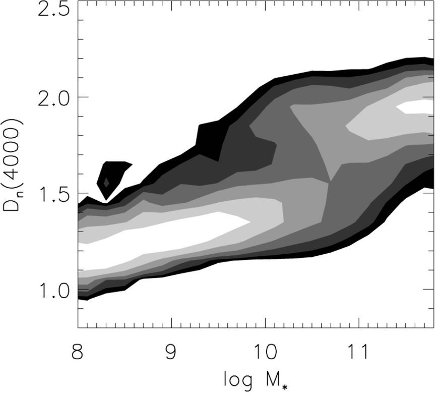
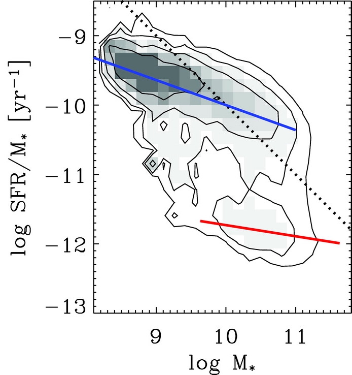
Figure 18.25: The bimodal galaxy distribution (left: Kauffmann et al. (2003b); right: Schiminovich et al. 2007).
In both panels, a clear bimodality in the SFR is observed (remember that \(D4000\) is anti-correlated with SFR). The figure on the left in particular makes it clear that there is quite a sharp transition at \(\approx 3\times 10^{10}\,M_\odot\) between star-forming galaxies at lower masses and quiescent galaxies at higher masses (Kauffmann et al. 2003b).
Correlating SFR with color and morphological properties shows that the tight star-forming sequence mostly corresponds to the blue cloud in the color–absolute-magnitude diagram, while the more diffuse mode with low sSFR matches the red sequence. Remarkably, ultraviolet observations that are sensitive to very low SFR demonstrate that many elliptical galaxies have low levels of star formation. Thus, the red-sequence/blue-cloud bimodality is, unsurprisingly, fundamentally one of low-vs-high SFR. That it is the spiral disks that are star-forming, while elliptical galaxies do not is made clear further when we split the sSFR vs. stellar mass distribution by Sérsic index \(n\): disk-like galaxies with \(n < 2.4\) are essentially only found in the blue cloud, while elliptical-like galaxies with \(n > 2.4\) are largely located in the red sequence (Schiminovich et al. 2007).
The exact appearance of the star-forming sequence (the blue cloud) in sSFR versus stellar mass holds important information about the overall evolution of star formation in the Universe (e.g., Brinchmann et al. 2004). The sSFR increases with decreasing stellar mass, indicating that lower-mass galaxies are presently forming a larger fraction of their mass than more massive galaxies. This is the first indication of a trend that we will discuss further below: star formation in the Universe appears to be shifting towards smaller galaxies as the Universe evolves, a phenomenon known as downsizing.
Investigating star formation in galaxies at higher redshift requires detailed observational data on large, statistical samples of galaxies at these redshifts. The easiest, although by no means easy, statistic to measure is the total star formation rate per unit comoving volume as a function of redshift. This can be done by using broad observational properties such as the integrated ultraviolet or far-infrared luminosities of galaxies, rather than requiring detailed spectra or spatially-resolved observations. The earliest determination of the cosmic star-formation history used chemical evolution modeling along the lines of Chapter 11.1, but applied to observations over cosmological volumes rather than of individual galaxies. By modeling the observed abundances of gas, heavy elements, and dust in massive, high-redshift disk galaxies, Pei & Fall (1995) found a rapid increase in the metallicity with decreasing redshift that is caused by high SFR at \(1 \lesssim z \lesssim 2\) compared to today. Thus, the overall cosmic SFR appeared to be much higher in the past than it is today. Lilly et al. (1996) confirmed this by measuring the ultraviolet luminosity density out to \(z \approx 1\) and finding that it increases steeply with redshift; they interpreted this increase as an increase in the cosmic SFR. Madau et al. (1996) extended this type of analysis to much higher redshift using observations from the Hubble Deep Field, finding evidence for a peak in the cosmic SFR somewhere between \(z=1\) and \(z=2\).
Nowadays, direct measurements of the cosmic SFR can be obtained by essentially applying the SPS modeling technique from Section 18.1 to match the ultraviolet and far-infrared luminosity density at different redshifts, because both the ultraviolet and far-infrared luminosities trace recent star formation (see Section 18.1.2). That is, rather than using SPS modeling to determine the SFH of an individual galaxy by matching its observed fluxes, we can use SPS modeling to determine the cosmic SFH by matching the observed luminosity density on cosmological scales. The review by Madau & Dickinson (2014) contains such a recent measurement and the resulting cosmic SFR that now extends out to \(z=8\) is shown in Figure 18.26.
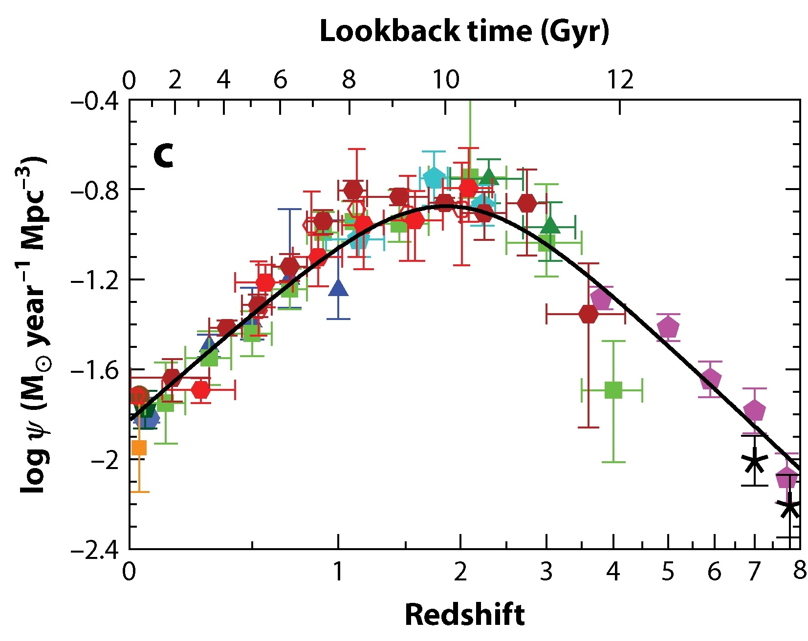
Figure 18.26: The cosmic star-formation history (adapted from Madau & Dickinson 2014).
This cosmic SFR shows a clear peak at \(z\approx 2\), known as cosmic noon. Overall, the SFR at cosmic noon was about an order of magnitude larger than it is today. With an average cosmic SFR of \(\approx 10^{-0.85}\,M_\odot\,\mathrm{yr}^{-1}\,\mathrm{Mpc}^{-3}\), galaxies formed \(\approx 1.4\times 10^8\,M_\odot\,\mathrm{Mpc}^{-3}\) of stars in the \(\approx 1\,\mathrm{Gyr}\) period between \(z=3\) and \(z=2\). This is about half of the \(z=0\) cosmic stellar mass density of \(\approx 2.2\times 10^8\,M_\odot\) that we estimated in Section 18.2 (see paragraph following Equation 18.21). Thus, about half of all the stellar mass in the Universe was created in a brief period around cosmic noon. This epoch is therefore one of the most interesting observationally to understand the formation and evolution of galaxies and cosmic noon is, therefore, a prime target for the next generation of space-based (e.g., JWST) and ground-based (extremely-large telescopes) surveys (Forster Schreiber & Wuyts 2020).
The cosmic SFR tells use the overall evolution of the SFR over cosmological volumes, but it does not explain how star formation proceeds within any individual galaxy nor can we derive from it the reason for the rise in the cosmic SFR from the early Universe to \(z\approx2\) and its subsequent fall towards the present. To elucidate this, it is necessary to look more closely at the distribution of SFR among galaxies at a range of redshifts. Low-redshift determinations of this show that it can be represented by a Schechter function of Equation (18.14) (e.g., Gallego et al. 1995), with a characteristic SFR of \(\mathrm{SFR}_* \approx 9\,M_\odot\,\mathrm{yr}^{-1}\) and a faint-end slope of \(\alpha = -1.5\) (Bothwell et al. 2011). Observations of the distribution of SFRs at higher redshift show that the distribution shifts towards higher SFR, with a significantly increased contribution from galaxies with very high SFR (Le Floc'h et al. 2005). Many of these high-SFR galaxies are luminous infrared galaxies (LIRGs; \(L_{\mathrm{FIR}} > 10^{11}\,L_{\mathrm{FIR},\odot}\)) or ultra-luminous infrared galaxies (ULIRGS; \(L_{\mathrm{FIR}} > 10^{12}\,L_{\mathrm{FIR},\odot}\)): galaxies with very high far-infrared (FIR) luminosities caused by high SFRs (up to \(100\,M_\odot\,\mathrm{yr}^{-1}\) and higher). Such galaxies are rare in the present Universe and they only contribute a small amount to the present cosmic SFR, but their abundance increases substantially at higher redshift where they contribute a significant amount of the cosmic SFR. This is again the effect of downsizing: SFR in the past occurred in larger, more massive galaxies than today.
To better understand the physics of galactic star formation requires us to investigate the dependence of the SFR in galaxies on other galactic properties. The most useful and popular such correlation is the Schmidt law (also known as the Kennicutt-Schmidt law, see below), which is a tight correlation between the SFR surface density \(\Sigma_{\mathrm{SFR}}\) (usually measured in units of \(M_\odot\,\mathrm{yr}^{-1}\,\mathrm{kpc}^{-2}\)) and the total surface density of gas \(\Sigma_{\mathrm{gas}}\) (usually measured in units of \(M_\odot\,\mathrm{pc}^{-2}\)). A correlation of the form \begin{equation}\label{eq-exgal-schmidt-general} \Sigma_{\mathrm{SFR}} \propto \Sigma_{\mathrm{gas}}^n\, \end{equation} was first proposed by Schmidt (1959), who argued that \(n\approx 2\) from observations of the density of gas, young stars, and white dwarfs in the solar neighborhood. This relation was observationally refined, first by Kennicutt (1989), who found \(n = 1.3 \pm 0.3\), and later by Kennicutt (1998b), who found \(n = 1.4 \pm 0.15\). The latter is still considered the standard value. Kennicutt based these \(n\) determinations on SFR determinations from the H\(\alpha\) line (see Section 18.1.2) and gas densities obtained from neutral hydrogen and molecular CO. The tight correlation between \(\Sigma_{\mathrm{SFR}}\) and \(\Sigma_{\mathrm{gas}}\) is clear in the left panel of Figure 18.27.
|
|
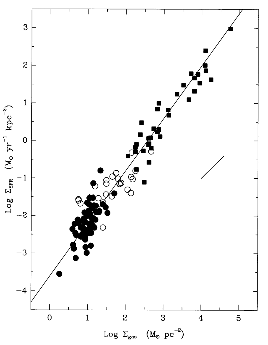
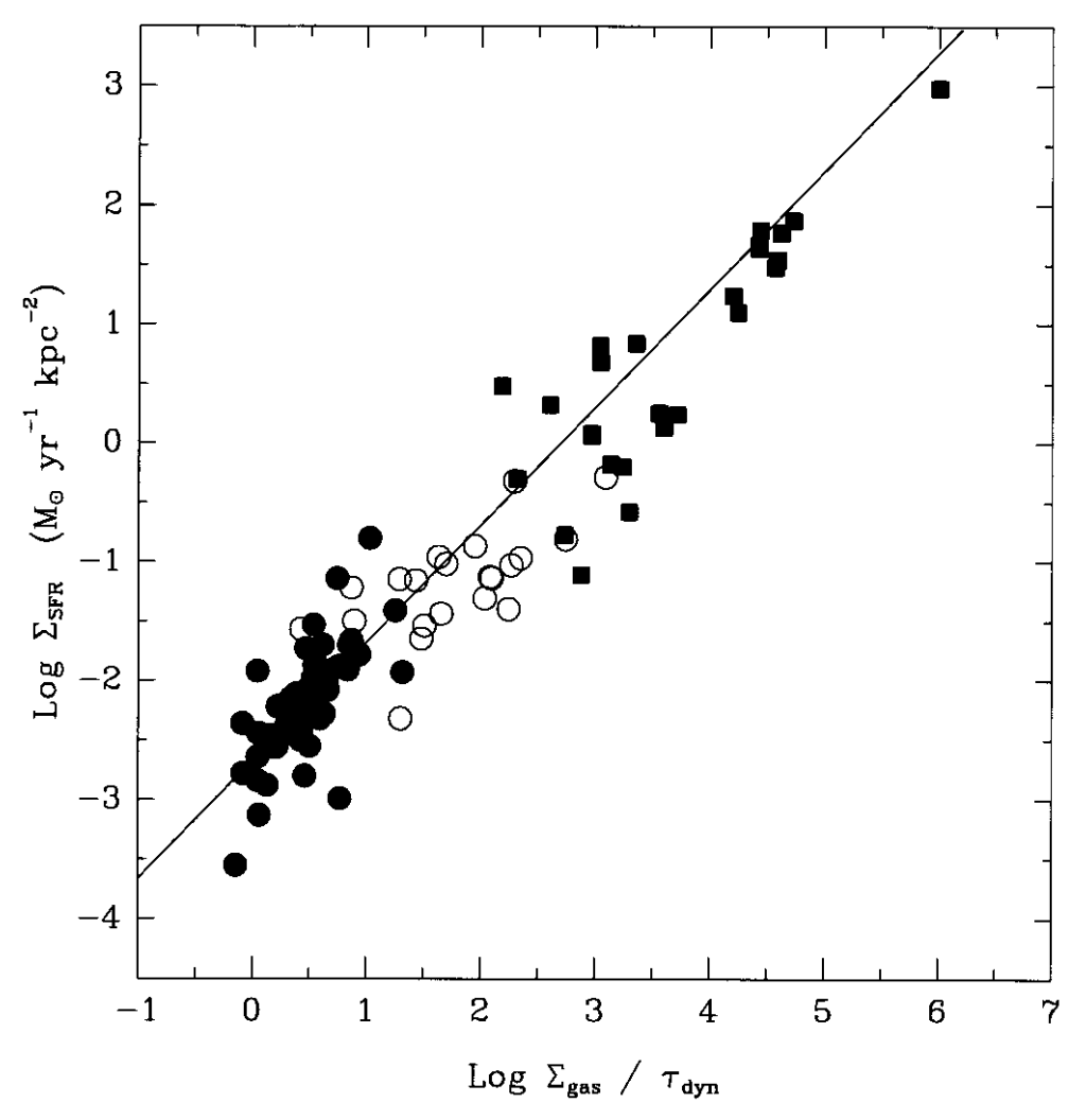
Figure 18.27: The Kennicutt-Schmidt law (Kennicutt 1998b): SFR density vs. gas density (left panel) and gas density divided by the dynamical time (right panel).
The star formation efficiency time scale \(\tau_*\) that we strongly relied on in Chapter 11.1 for building theoretical models of chemical evolution is defined in Equation (11.10) as \(\tau_* = M_g/\dot{M}_*\), where \(M_g\) is the total gas mass and \(\dot{M}_*\) the SFR. The time scale \(\tau_*\) gives the time it takes to consume the available gas at the current SFR. Dividing numerator and denominator by the area of the galaxy and using the Schmidt law from Equation (18.39), we have that \begin{equation}\label{eq-exgal-schmidt-general-astaustar} \tau_* = {\Sigma_{\mathrm{gas}}\over \Sigma_{\mathrm{SFR}}} \propto \Sigma_{\mathrm{gas}}^{1-n}\,. \end{equation} Thus, a constant star-formation efficiency time scale corresponds to \(n=1\) and the observed value of \(n = 1.4\pm 0.15\) therefore implies a non-constant \(\tau_*\) that instead decreases with increasing gas mass. It, therefore, appears that galaxies with higher gas masses use up their gas supply faster.
Observations of the Schmidt law at higher redshifts are complex, largely because of the uncertainty in determining the molecular gas masses in these galaxies (Carilli & Walter 2013). Using reasonable assumptions on how to convert the CO luminosity to a molecular gas mass (the so-called \(X_{\mathrm{CO}}\) factor), it appears that there is a different Schmidt law at \(z\approx 2\) for starburst galaxies (with particularly high SFR) and normal star-forming galaxies, with the former consuming gas through star formation at a rate that is about an order of magnitude faster (Genzel et al. 2010; Daddi et al. 2010). However, this interpretation is strongly dependent on the assumed \(X_{\mathrm{CO}}\) factor, which in these analyses is assumed to be different for starburst and normal galaxies, giving rise to the difference in Schmidt laws. As we will see below, the difference between high-redshift starburst and normal galaxies disappears in an alternative, more physical statement of the Schmidt law.
The Schmidt law that we have discussed so far concerns entire galaxies: both the SFR and total-gas surface densities are those of entire galaxies. However, using resolved observations of the SFR and gas content of galaxies, we can also investigate the existence of a Schmidt law for smaller, sub-kpc regions of galaxies (down to 30 to 50 pc in the Local Group). The result of a comprehensive analysis of this type is shown in Figure 18.28.
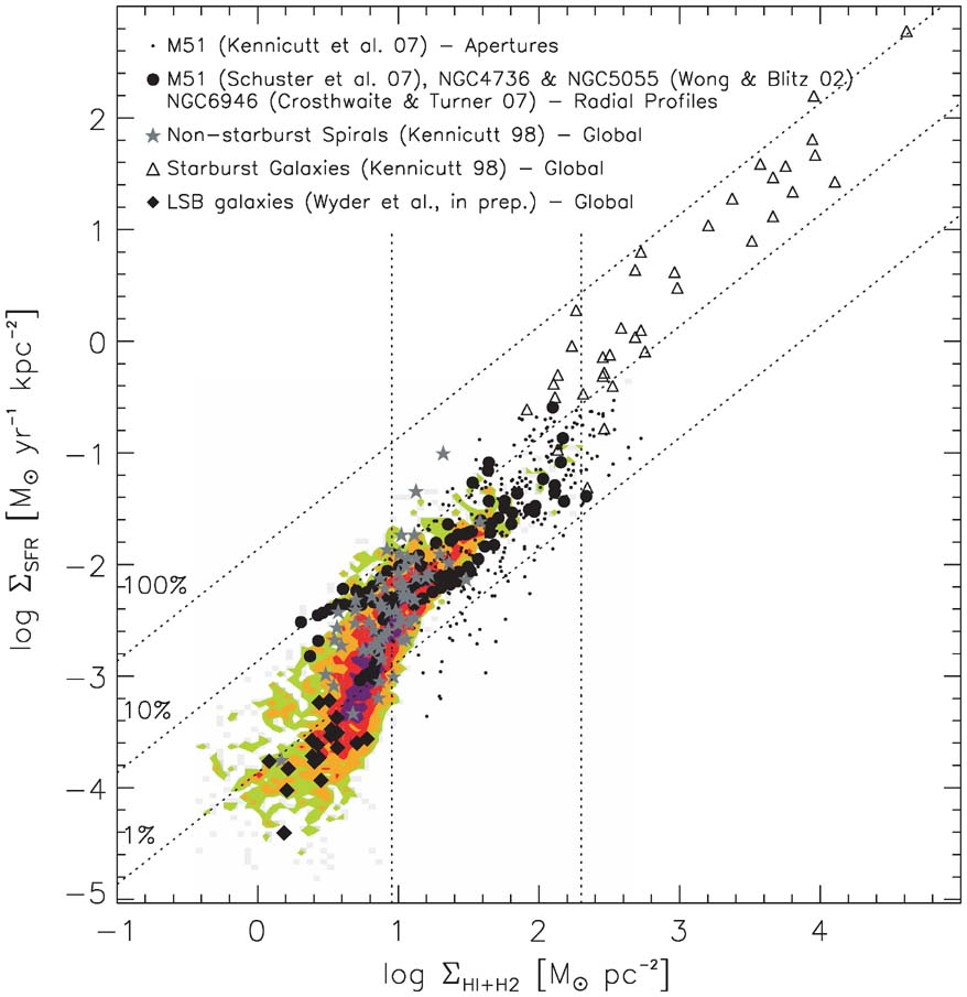
Figure 18.28: The Schmidt law for sub-kpc regions of galaxies (Bigiel et al. 2008; the gray diagonal lines reflect constant star-formation efficiency time scales).
At the higher gas density end where the distribution of local and global densities overlap, the local and global Schmidt laws agree. There, thus, appears to be a single Schmidt law that relates SFR and gas density. This makes it plausible that the Schmidt law is a physically-meaningful law about how gas turns into stars, rather than yet another galactic scaling relation. However, the full local+global Schmidt law does not conform to a single power-law of the form of Equation (18.39), but instead displays a break at a gas density of \(\approx 10\,M_\odot\,\mathrm{pc}^{-2}\). Below this break, the SFR density steeply declines with gas density.
The likely reason for the \(\approx 10\,M_\odot\,\mathrm{pc}^{-2}\) break becomes clear when instead of plotting SFR density vs total gas density, we look at the correlation of the SFR density with just the molecular gas density. A tight correlation between these two exists as well and, moreover, the power-law index of their relation is \(n \approx 1\), that is, they are linearly correlated (Bigiel et al. 2008; Schruba et al. 2011). The relation between SFR and molecular gas density also does not display a break. Detailed observations of star-forming regions show that star formation happens in dense molecular clouds, with stars forming from dense molecular clumps within these clouds. Inside molecular clouds, there is a strong linear correlation between the number of young stars and the number of high-density clumps (e.g., Lada et al. 2010). Thus, the linear correlation between SFR density and molecular gas density is not surprising, although it is surprising that the correlation extends all the way from very low SFRs to the SFRs observed in starburst galaxies (Wu et al. 2005; Lada et al. 2012). It, therefore, appears that dense molecular gas is fundamental for star formation (Krumholz & McKee 2005). This then explains the break in the Schmidt law when considered as a function of total gas mass: \(\approx 10\,M_\odot\,\mathrm{pc}^{-2}\) is the threshold below which gas cannot efficiently cool to molecular form, making the formation of dense molecular clouds difficult and, therefore, inhibiting star formation.
There is, however, another reformulation of the standard Schmidt law that produces as clean a physical picture, but for very different reasons. Considering the SFR density not as a function of the total gas density alone, but instead as a function of the total gas density divided by the dynamical time, we find as tight of a correlation as the original Schmidt law. This is shown in the right panel of Figure 18.27. The line that is shown in the figure is a linear fit, which provides a good fit to the data. That is, the SFR density approximately satisfies \(\Sigma_{\mathrm{SFR}} \propto {\Sigma_{\mathrm{gas}}/ \tau_\mathrm{dyn}}\), where \(\tau_\mathrm{dyn}\) is the dynamical time. The constant of proportionality of this relation is such that the SFR is \(\approx 10\%\) of the available gas per orbit. This type of relation is expected in theories where star formation happens because of global dynamical instabilities, such as bar or spiral-arm formation and density-compressions created by their effect (e.g., Silk 1997; Ostriker et al. 2010). The reason for the normal Schmidt law in this picture is that \(\tau_\mathrm{dyn} \approx \rho^{-1/2}\) (Equation 2.28) and in galaxies approximately \(\rho \propto \Sigma_{\mathrm{gas}}\), leading to the observed \(n \approx 1.5\).
Thus, we end up with two competing pictures for what drives galactic star formation. One is a local picture, where star formation occurs from dense molecular gas on small scales (\(\lesssim 100\,\mathrm{pc}\), the size of the largest molecular clouds) through a combination of cooling, turbulence, and eventually feedback from massive formed stars disrupting the star-forming cloud and preventing it from forming more stars. The global view takes the opposite approach and sees star formation in galaxies being largely driven by large-scale effects: mergers, spiral arm formation and shocks, etc. The true picture of star formation likely combines both approaches: global, large-scale events cause gas to compress over large areas of a galaxies, leading to efficient formation of dense molecular gas that quickly cools down to very high densities and forms stars in a large number of small, localized clouds.
The phenomenological account of star formation that we have presented here misses a large amount of external context. We discussed how the star formation efficiency is such that \(\approx 10\%\) of the available gas mass is turned into stars each orbit. Simulations show that this is both quite inefficient, in that without significant heating of the star-forming medium many more stars would be born from the available gas, and efficient, in the sense that galaxies are \(\gg 10\) orbits old and they should therefore have consumed all of their gas a long time ago if it was not replenished. Thus, significant inflows of gas over time are required to sustain star formation, while the heating that causes the inefficiency of star formation is likely accompanied by significant outflows of gas. This agrees with our conclusion from the chemical-evolution modeling of the solar neighborhood in Chapter 11.2.4.

 .
. .
. .
.