← Previous section Next section →

18.1. Stellar-population synthesis modeling

\label{sec-exgal-sps}

18.1.1. Photometry and spectroscopy

\label{sec-exgal-sps-photspec}

Essentially all observations of galaxies are at their core flux measurements of some part of the electromagnetic spectrum. These can either be obtained through spectroscopy as flux densities—flux per unit wavelength—by using a prism or grating to produce a spectrum, or they are fluxes obtained by integrating the flux density over a wavelength range using a filter, which can be broad or narrow, in a process called photometry. For external galaxies, fluxes can be integrated over the entire or a large part of the galaxy (or not) and spectra can be taken at a single location, along a one-dimensional line (often the major axis), or covering the full two-dimensional area of the galaxy (as in integral-field spectroscopy). Units of flux density are \(\mathrm{W\,m}^{-3}\) in SI units, but SI units are hardly used in astrophysics, so instead spectra are reported in units of, for example, \(\mathrm{erg\,cm}^{-2}\,\mathrm{s}^{-1}\,\AA^{-1}\) (in the optical; e.g., SDSS), or, when considering flux per unit frequency instead of per unit wavelength, Jansky (in the radio). The fluxes measured in photometry have units of \(\mathrm{W\,m}^{-2}\) in SI units, but are again typically expressed using units such as \(\mathrm{erg\,cm}^{-2}\,\mathrm{s}^{-1}\). More importantly, photometric fluxes are usually expressed as magnitudes, a unitless, logarithmically-scaled version of flux defined using a reference flux as \begin{equation}\label{eq-exgal-magdef} m = -2.5\,\log_{10}\left(f/f_\mathrm{ref}\right)\,, \end{equation} where \(f\) is a source’s flux in a given photometric band and \(f_\mathrm{ref}\) is the reference flux in that band. Commonly used reference fluxes are Vega (i.e., the flux of the star Vega in the given band) or the AB system (Oke & Gunn 1983). The definition of magnitude is such that fainter sources have larger magnitudes.

Optical spectrographs with CCD detectors can readily measure spectra from the ground over the entire visible range from the UV cut-off at \(\approx 3100\,\AA\), below which the atmosphere is opaque, to \(\approx 1\,\mu m\). Spectroscopy in the near-infrared extends in certain windows out to \(\approx 15\,\mu m\) from the ground, but requires space-based detectors at longer wavelengths to observe the mid- and far-infrared regions. Sub-millimeter and millimeter spectra can be obtained from the ground in many windows (e.g., by ALMA) and the radio range is fully accessible from the ground from about 1 cm to about 10 m, above which it is blocked by the ionosphere. Atmospheric transmission at wavelengths longer than \(\approx 1\,\mu m\) is strongly affected by water vapor, which is why ground-based infrared, (sub-)millimeter, and sensitive radio telescopes are best constructed in dry locations.

High-resolution spectra—spectra with fine wavelength sampling—give the most possible information about a celestial source. The resolution of spectrographs is conventionally defined as \(R = \lambda / \Delta \lambda\). Opinions differ on exactly where to draw the line between different categories, but roughly spectra with \(200 \lesssim R \lesssim 3,000\) are low resolution, \(3,000 \lesssim R \lesssim 10,000\) are medium resolution, and those with \(R \gtrsim 10,000\) are high resolution (at least in the optical and near infrared); at resolutions \(\lesssim 200\) we generally speak of a spectral energy distribution (SED) and then the exact filter used over a resolution element’s wavelength range matters for the physical interpretation of the observation. For stars, optical and near-infrared spectra at high resolution allow the determination of precise line-of-sight velocities, stellar rotation velocities, and the abundances of many elements. For external galaxies, however, the internal velocity dispersion \(\sigma\) smooths out high-resolution structure and galaxy spectra have at best an effective resolution of \(R \approx c / \sigma\), where \(c\) is the speed of light. For massive galaxies, this is \(R \approx 3000/(\sigma / 100\,\mathrm{km\,s}^{-1})\). For most purposes, there is therefore little reason to obtain a medium- or high-resolution spectrum of a massive galaxy. Most spectroscopic galaxy surveys (e.g., SDSS) therefore have resolutions of \(R \approx 2,000\) to \(4,000\).

While spectra contain more information than broadband or narrowband photometry, spectra are currently difficult to obtain for large numbers of sources or for faint sources. Photometry, however, can be determined for large numbers of sources from imaging and photometry can be obtained for faint sources that are orders of magnitudes fainter than the sources for which we can easily obtain spectra. Broadband filters have \(R \approx\) a few: In the optical, broadband filters have widths of \(\approx 1000\,\AA\), while in the near-infrared they have widths of \(\approx 0.4\,\mu m\). They are generally designed to avoid regions of strong atmospheric absorption. Narrow-band filters have a wide range of widths, but in the optical are typically somewhere between \(50\,\AA\) and \(200\,\AA\) (e.g., the Strömgren photometric system). Narrow-band filters are useful for measuring fluxes of absorption (for stars) or emission lines (for nebular emission from external galaxies). In external galaxies, the most commonly-used of these are narrowband filters designed to capture the star-formation-tracing H\(\alpha\), H\(\beta\), and \([\mathrm{O\,II}]\) line flux produced by ionized gas surrounding young, massive stars (see below).

18.1.2. Generalities

\label{sec-exgal-sps-general}

We directly observe spectral flux densities or photometric fluxes (or magnitudes), but astrophysically-relevant external-galaxy properties are quantities such as stellar mass, the present and historical star-formation rate, the gas mass, the stellar and baryonic mass-to-light ratio, the metallicity of the interstellar medium and of stars, the two- and three-dimensional shape of galaxies, and their decomposition into different components. These can be determined for a galaxy as a whole or as a function of location within the galaxy. And they all have to be determined from observations of flux densities or fluxes. Much of the success of extragalactic astronomy in piecing together the formation and evolution of different types of galaxies stems from the great and concerted effort by many researchers to develop a variety of tools for determining intrinsic galaxy properties from observational data. We have already in detail discussed the determination of galaxy light profiles and shapes and their decomposition into different components in previous chapters, so we will focus on star formation rates and histories, stellar masses, mass-to-light ratios, and chemical composition here.

Of all of the intrinsic galaxy properties of interest, the measurement of the instantaneous (\(\lesssim 10\,\mathrm{Myr}\)) star-formation rate (SFR) requires in some sense the least amount of modeling. A burst of star formation causes the formation of massive stars with lifetimes \(\lesssim 10\,\mathrm{Myr}\). These stars are very luminous and dominate the UV spectrum of a galaxy, but they also ionize gas surrounding them, causing it to glow through recombination in emission lines such as H\(\alpha\), H\(\beta\), and \([\mathrm{O\,II}]\), and to heat dust grains in the interstellar medium, giving rise to far-infrared emission. All of these (and more, see Kennicutt & Evans 2012 for a review) can be used to determine the instantaneous SFR in an external galaxy. Because of the ubiquity of optical spectroscopy and narrow-band photometry and because of their relatively-unambiguous nature, the emission-line tracers are the most commonly used ones. Massive young stars are able to ionize their surrounding gas if they have masses exceeding \(\approx 15\,M_\odot\) with, for a standard initial mass function (IMF) of formed stars in a star-formation event, the greatest contribution coming from \(\approx 30\) to \(40\,M_\odot\) (Kennicutt & Evans 2012). All of these stars have lifetimes \(\lesssim 10\,\mathrm{Myr}\) and thus trace the instantaneous SFR. To relate an observed emission-line flux to a SFR requires a calibration exercise, which is typically performed using the stellar-population synthesis technique that we discuss below, by simulating the emission-line flux of full young stellar populations of a given age distribution, metallicity, and initial mass function. For example, for the H\(\alpha\) emission line, we have that (Murphy et al. 2011) \begin{equation}\label{eq-exgal-halpha-sfr} {\mathrm{SFR} \over M_\odot\,\mathrm{yr}^{-1}} = {L_{\mathrm{H}\alpha} \over 1.86\times 10^{41}\,\mathrm{erg\,s}^{-1}}\,, \end{equation} where \(L_{\mathrm{H}\alpha}\) is the H\(\alpha\) emission line’s luminosity, equal to \(4\pi\,D^2\) times the flux, where \(D\) is the distance (the luminosity distance on cosmological scales; see Chapter C.4.3). The Milky Way, which is steadily forming new stars for many Gyr, has a SFR of \(\approx 2\,M_\odot\,\mathrm{yr}^{-1}\) (Licquia & Newman 2015), while starburst galaxies can have SFRs of \(\mathcal{O}(100\,M_\odot\,\mathrm{yr}^{-1})\) (e.g., da Cunha et al. 2010).

To determine stellar masses and stellar mass-to-light ratios from observed fluxes and flux densities requires one to infer the entire history of star formation and essentially add up all of the stellar mass formed over the lifetime of a galaxy. Thus, we need to determine or at least constrain the full star-formation history (SFH) of a galaxy and use it to determine the total stellar mass or to relate the stellar mass-to-light ratio to observed properties such as colors. In essence, all measurements of the SFH from the emission of stars use the fact that stars with different initial masses have both different lifetimes, spanning all the way from \(\approx 5\,\mathrm{Myr}\) to trillions of years, and emit light with different spectral energy distributions: short-lived, hot, massive stars emit largely at shorter wavelengths, while long-lived, cooler, low-mass stars radiate at longer wavelengths, because of Wien’s law. Thus, by decomposing a galaxy’s spectrum or SED into contributions from high- and low-mass stars with their associated lifetimes, we can determine the SFH: assuming an IMF, the number of high-mass stars tells us how many stars formed since the time that is equal to their lifetime, and extending this procedure to lower-mass stars allows us to determine the number of stars formed to earlier and earlier epochs and thus establish the full SFH. In the Milky Way, with resolved stars, this conceptual procedure can be implemented almost exactly by determining volume densities of stars of different initial masses (e.g., Dolphin 2002; Bovy 2017b), but in external galaxies we need to model the composite spectrum or SED that results from adding up all flux contributions and match it to observations to determine the SFH. This modeling of the composite spectrum or SED is called stellar population synthesis or SPS.

At a basic level, we can approximate stellar spectra as blackbodies and the composite spectrum of a galaxy with high recent star formation then has significant UV and blue emission coming from short-lived massive stars, while the spectrum of a galaxy consisting largely of old stars is tilted towards the red and infrared because of the predominance of cool, low-mass stars. A galaxy’s observed color is therefore a direct, if rough, indicator of its star formation history. However, SPS is most powerful when applied to detailed galaxy spectra and while the spectra of very massive stars are well represented by the smooth black-body radiation law (aside from absorption lines of hydrogen and helium), the spectra of most stars are not featureless black-body curves. Instead, they display abundant absorption features due to atoms, both neutral and ionized, of different chemical elements as well as, at lower temperatures, molecules in the stellar photosphere. Rather than being an impediment to determining the SFH, they are in fact a great help, as the depth of some prominent absorption features can give a clear indication of the age and metallicity distribution of a galaxy. To start off a discussion of more realistic SPS modeling, let’s first look at some integrated spectra of different types of external galaxies in Figure 18.1: elliptical, spiral, and irregular.

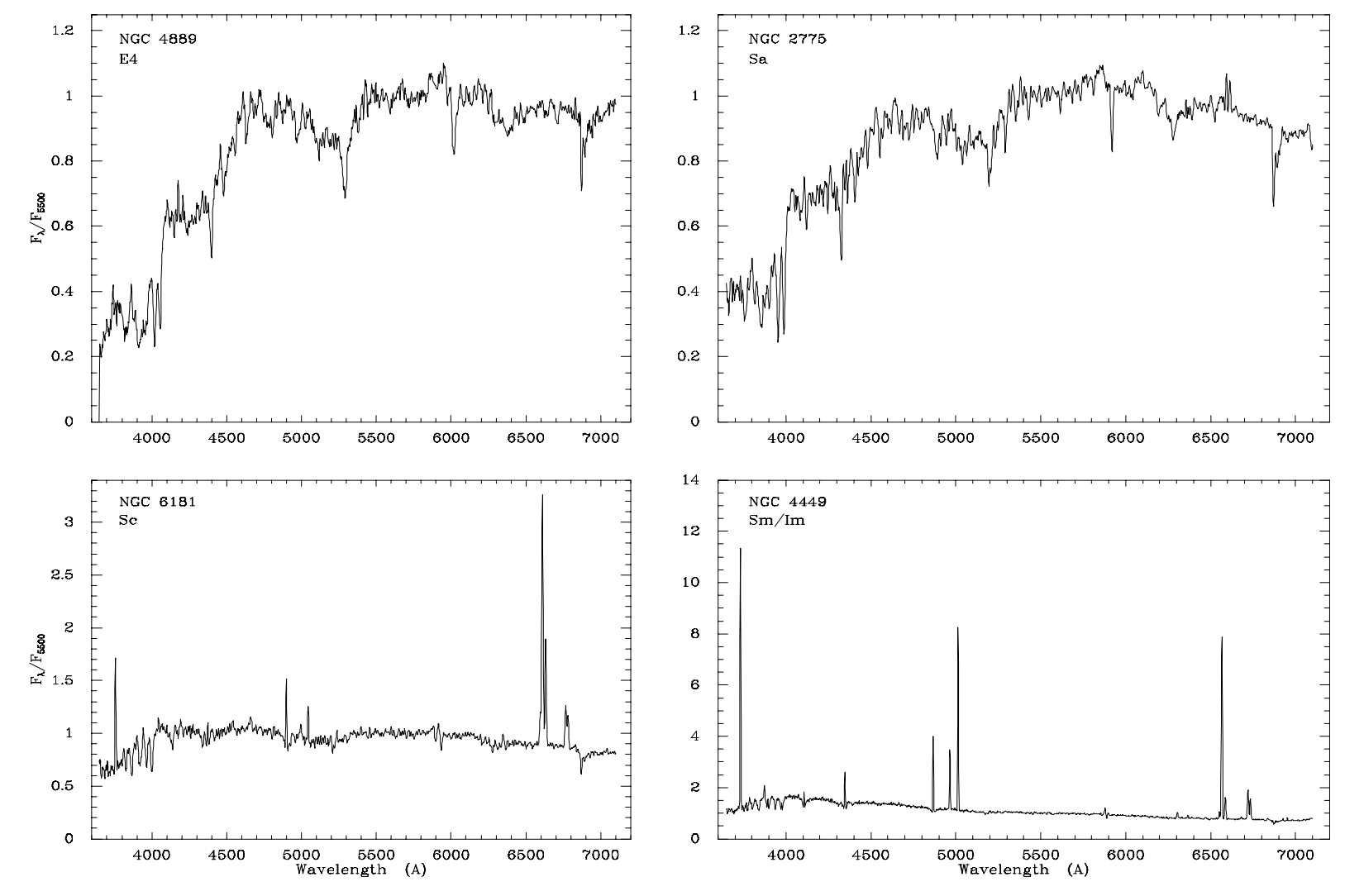
Figure 18.1: Sample spectra of elliptical [top left], spiral [top right and bottom left], and irregular galaxies [bottom right] (Kennicutt 1998a; originally presented in Kennicutt 1992).

The top row shows typical spectra of ellipticals and early-type spirals (see the discussion of the Hubble sequence in Section 18.3 below), while the bottom row displays typical spectra of late-type spirals and irregular galaxies. It is clear that these are not simple black-body curves! The spectra of elliptical and early-type galaxies are dominated by ubiquitous absorption lines and their spectra are in fact quite similar. Thus, even though these galaxies are morphologically very different, they have similar SFHs. The spectra of late-type spirals and irregular galaxies have less prominent absorption features, due to the presence of larger numbers of young, massive, hot stars, and they also have strong emission lines from gas ionized by the ultraviolet emission of massive stars (see the discussion of H\(\alpha\) etc. above), although emission lines can also be created by the ionizing radiation from active galactic nuclei.

The absorption features in the integrated spectra of external galaxies contain much information about their SFH and metallicity distribution. For example, a particularly useful feature is the break at \(\approx4000\,\AA\) that is very clear in the top row of Figure 18.1. This is called the \(4000\,\AA\) break and it is a strong break in the spectrum that results from a confluence of many absorption features in the photospheres of cool stars (roughly, cooler than the Sun). Prominent lines from Ca combine with some of the Balmer lines, a band of molecular CN absorption, and a host of other metal lines to create a dense pattern of absorption lines that appears as a break blueward of \(4000\,\AA\) (the appearance of the break from the dense set of absorption features is often referred to as line blanketing; Wildey et al. 1962; Gorgas et al. 1999). Because this only happens in cool stars, the depth of the break is an indication of the relative number of cool stars to hot stars, or of old to young stellar populations, and is, therefore, an indicator of the galaxy’s SFH. The elliptical and early-type-spiral spectra displayed above have a prominent, deep \(4000\,\AA\) break, indicating that they are dominated by cool, old stars. An indicator \(D4000\) of the strength of the break can be defined by comparing the average flux density above and below the location of the break (e.g., Bruzual 1983; Balogh et al. 1999) and both SPS modeling (Bruzual 1983; Hamilton 1985) and comparisons with other tracers of star formation (e.g.. Dressler & Shectman 1987) demonstrate that \(D4000\) traces the contribution from old stars well. As an absorption indicator, it is dependent on the chemical composition of the radiating stars as well and it can therefore not be a fully unambiguous tracer of the SFH. Other break indicators of the SFH or the instantaneous SFR exist, with one of the other interesting ones being the Lyman break at at the Lyman limit of \(912\,\AA\). As a rest-frame ultraviolet feature, it traces the contribution from hot, massive stars and thus the instantaneous SFR. A break occurs in this case because light at wavelengths below the Lyman limit ionizes hydrogen with an electron in its ground state and this light is therefore efficiently absorbed by the gas surrounding the massive stars and by the intergalactic medium (Steidel et al. 1996).

18.1.3. Single stellar populations

\label{sec-exgal-sps-ssp}

While individual absorption features such as the \(4000\,\AA\) break are useful to obtain a rough, qualitative understanding of a galaxy’s SFH, quantitative constraints require full SPS modeling of the stellar populations in a galaxy. The basic structure of all SPS modeling is to break up a galaxy’s history and evolution into single stellar populations (SSPs), which represent the properties and evolution of stars of a given age \(\tau\) and metallicity \(Z\) (SPS generally does not consider additional population properties, for example, deviations from solar abundance ratios for certain elements; see Chapter 11.3). SSPs are combined to form a full galaxy by assuming an SFH and the evolution of \(Z\) with time, although \(Z\) is typically assumed to be constant. Additionally, the impact of dust attenuation and dust emission (especially important at \(\lambda \gtrsim 10\,\mu m\)) and of line emission from ionized gas clouds may be added to the resulting spectrum. The final galaxy spectrum can then either be directly compared to an observed galaxy spectrum or it may be integrated over narrow or broad photometric bands to predict to observed photometry. Aside from directly modeling the observed spectrum, SED, or photometry of a galaxy, SPS modeling can also be used to derive simple relations between quantities such as the mass-to-light ratio or a galaxy’s mean age and observed properties such as colors, spectral indicators like \(D4000\), and others.

The generation of model SSPs is one of the main ingredients of SPS modeling and one that has received much attention in the decades since SPS was first conceived in the pioneering works of Tinsley (1968), Searle et al. (1973), and Tinsley & Gunn (1976). The basic ingredients of an SSP model are (i) a model for the IMF, (ii) stellar evolutionary tracks, and (iii) a library of spectra or SEDs of stars spanning all possible stellar types and the full wavelength range of the relevant observations. We discuss these three ingredients in more detail in the following paragraphs.

A model for the IMF gives the distribution of star masses when a solar mass of gas turns into a solar mass of stars in a star-formation event. Typically, the IMF is assumed to be universal, that is, it does not depend on additional parameters such as metallicity or the properties of the galaxy the gas resides in. Thus, the IMF is given by a function \(\Phi(M)\) which gives the number of stars \(\mathrm{d}N\) of stars in a range of mass \(\mathrm{d}M\): \begin{equation} \Phi(M) = {\mathrm{d} N \over \mathrm{d} M}\,. \end{equation} This is the definition that we will adopt here, but note that it is also common in the literature to define the IMF in logarithmic bins in mass, in particular, \(\xi(\log_{10} M) = \mathrm{d} N / \mathrm{d} \log_{10} M\). These are related as \(\xi(\log_{10} M) = M\ln 10\,\Phi(M)\). The most popular IMF models are those of Chabrier (2003) and of Kroupa (2001). The classical power-law IMF \(\Phi(M) \propto M^{-2.35}\) from Salpeter (1955) is not typically used, because it does not represent the IMF well at the low-mass end (\(M \lesssim 1\,M_\odot\)), where it predicts too many low-mass stars compared to solar-neighborhood observations. This matters, because most of the stellar mass in a galaxy is locked up in low-mass stars. A variety of other IMF shapes are used and they are generally characterized by comparing their initial-mass distributions to the classical Salpeter (1955) form: bottom-heavy IMFs predict more low-mass stars than the Salpeter form (and, thus, many more compared to the canonical Chabrier 2003 and Kroupa 2001 forms), while bottom-light IMFs predict fewer low-mass stars; similarly, top-heavy and top-light IMFs predict more or less high-mass stars than the Salpeter IMF (Dave 2008). Figure 18.2 shows the IMF (in the form of \(\xi(\log_{10} M)\)) and the cumulative IMF for all three models when normalizing the IMF to one solar mass between \(0.079\,M_\odot\) and \(100\,M_\odot\).

def dNdm_chabrier2003(m):
    # Unnormalized dn/dm
    tm= m.to_value(u.Msun)
    out= numpy.empty_like(tm)
    indx= tm < 1.
    out[indx]= 0.158/tm[indx]*numpy.exp(-numpy.log10(tm[indx]/0.079)**2./2./0.69**2.)
    out[True^indx]= (m[True^indx])**-2.3*0.158*numpy.exp(-numpy.log10(0.079)**2./2./0.69**2.)
    return out
def dNdm_kroupa2001(m):
    # Unnormalized dn/dm
    tm= m.to_value(u.Msun)
    out= numpy.empty_like(tm)
    out[(tm < 0.08)]= (tm[(tm < 0.08)]/0.08)**-0.3
    out[(tm >= 0.08)*(tm < 0.5)]= (tm[(tm >= 0.08)*(tm < 0.5)]/0.08)**-1.3
    out[(tm >= 0.5)]= (tm[(tm >= 0.5)]/0.5)**-2.3*(0.5/0.08)**-1.3
    return out
def dNdm_salpeter1955(m):
    # Unnormalized dn/dm
    tm= m.to_value(u.Msun)
    return tm**-2.35
from scipy import integrate
def cumul_imf(m,imf):
    return integrate.quad(lambda x: imf(10.**x*u.Msun)*10.**x,
                          numpy.log10(0.079),
                          numpy.log10(m.to_value(u.Msun)))[0]
ms= numpy.geomspace(0.079,100.,201)*u.Msun
from matplotlib.ticker import FuncFormatter
figure(figsize=(8,4))
subplot(1,2,1)
norm_chab= cumul_imf(100.*u.Msun,dNdm_chabrier2003)
loglog(ms,dNdm_chabrier2003(ms)*ms.to_value(u.Msun)/norm_chab,
       label=r'$\mathrm{Chabrier\ (2003)}$')
norm_krou= cumul_imf(100.*u.Msun,dNdm_kroupa2001)
loglog(ms,dNdm_kroupa2001(ms)*ms.to_value(u.Msun)/norm_krou,
       label=r'$\mathrm{Kroupa\ (2001)}$')
norm_salp= cumul_imf(100.*u.Msun,dNdm_salpeter1955)
loglog(ms,dNdm_salpeter1955(ms)*ms.to_value(u.Msun)/norm_salp,
       label=r'$\mathrm{Salpeter\ (1955)}$')
legend(frameon=False,fontsize=13.);
xlabel(r'$M / M_\odot$')
ylabel(r'$\mathrm{d} N / \mathrm{d} \log_{10} M$')
gca().xaxis.set_major_formatter(FuncFormatter(
                lambda y,pos: (r'${{:.{:1d}f}}$'.format(int(\
                    numpy.maximum(-numpy.log10(y),0)))).format(y)))
# Cumulative
subplot(1,2,2)
semilogx(ms,[cumul_imf(m,dNdm_chabrier2003)/norm_chab for m in ms])
semilogx(ms,[cumul_imf(m,dNdm_kroupa2001)/norm_krou for m in ms])
semilogx(ms,[cumul_imf(m,dNdm_salpeter1955)/norm_salp for m in ms])
xlabel(r'$M / M_\odot$')
ylabel(r'$N(<m)$')
gca().xaxis.set_major_formatter(FuncFormatter(
                lambda y,pos: (r'${{:.{:1d}f}}$'.format(int(\
                    numpy.maximum(-numpy.log10(y),0)))).format(y)))
tight_layout();

Figure 18.2: The Chabrier (2003), Kroupa (2001), and Salpeter (1955) IMFs.

We see that all three IMFs have the same high-mass behavior and that the Chabrier (2003) and Kroupa (2001) are essentially the same over the full mass range.

Stellar evolutionary tracks from stellar models are used to obtain the properties of stars of initial mass \(M\) at age \(\tau\) and metallicity \(Z\) that are necessary to model their spectra or SEDs. These models also provide other important properties of stars that are required to model galaxies, such as how much of their initial mass has been returned to the interstellar medium by age \(\tau\), whether stars have become stellar remnants (white dwarfs, neutron stars, and black holes) or not and, if they have, what the mass of the remnant is. The most important parameters for predicting the spectrum or SED of a star of a given age and metallicity are its effective temperature \(T_{\mathrm{eff}}\) and surface gravity \(\log g\). Because for SPS modeling, we are interested in the properties of stars of different initial masses at a given age \(\tau\), stellar evolutionary tracks—which describe the evolution of a star with mass \(M\) and metallicity \(Z\) over time—are converted to isochrones. Popular isochrone libraries include the PARSEC database (Girardi et al. 2000; Bressan et al. 2012; Marigo et al. 2017), the MIST library (Choi et al. 2016), the BaSTI models (Pietrinferni et al. 2004), and the Geneva tracks for high-mass stars (Schaller et al. 1992; Meynet & Maeder 2000).

As an example, we have extracted PARSEC isochrones on a logarithmic grid in ages from 100,000 yr to 10 Gyr using v3.6 of their web interface. We have done this for the set of metallicities \([\mathrm{M/H}]\) used in the SPS models of Bruzual & Charlot (2003) that we discuss below. The following code downloads and reads the isochrones:

import sys
import os
from pathlib import Path
import shutil
import tempfile
import subprocess
import gzip
from astropy.table import QTable
_CACHE_BASEDIR= Path(os.getenv('HOME')) / '.galaxiesbook' / 'cache'
_PARSEC_DIR= 'parsec'
_CACHE_PARSEC_DIR= _CACHE_BASEDIR / _PARSEC_DIR
_ERASESTR= "                                                                                "
def read_parsec(logage='all',metal_str='m62',
                Mmax=100.,pms=True):
    """Read PARSEC isochrones for a single age or
    a range of ages for a given metallicity.

    Possible logages are 5-10.3 with 0.1 increments

    Possible metal_str follow Bruzual & Charlot:
        m22: Z= 0.0001
        m32: Z= 0.0004
        m42: Z= 0.004
        m52: Z= 0.008
        m62: Z= 0.02
        m72: Z= 0.05
        m82: Z= 0.10

    Mmax= (100.) maximum initial mass in Msun

    pms= (True) if False, remove the pre-main sequence
                (using 'label', but note that this
                 doesn't work great)"""
    basename= f'parsec_{metal_str}.dat.gz'
    filePath= _CACHE_PARSEC_DIR / basename
    if not filePath.exists():
        download_parsec_file(basename)
    # Now read the data
    data= numpy.loadtxt(filePath)
    # Also read the column names, need to find these as
    # the line before the data starts
    with gzip.open(filePath,'r') as parsecfile:
        previous_line= None
        this_line= parsecfile.readline().decode()
        while this_line[0] == '#':
            previous_line= this_line
            this_line= parsecfile.readline().decode()
    names= previous_line[1:].strip().split()
    out= QTable(data,names=names)
    indx= (out['Mini'] < Mmax)
    indx= indx*(numpy.fabs(out['label']) > 0.01) \
        if not pms else indx
    if not logage == 'all':
        indx*= numpy.fabs(out['logAge']-logage) < 0.01
    return out[indx]
def download_parsec_file(basename):
    filePath= _CACHE_PARSEC_DIR / basename
    if filePath.exists(): return None
    try:
        # make all intermediate directories
        os.makedirs(filePath.parent)
    except OSError: pass
    sys.stdout.write('\r'+"Downloading file %s ...\r" \
                         % (filePath.name))
    sys.stdout.flush()
    # Safe way of downloading
    downloading= True
    interrupted= False
    file, tmp_savefilename= tempfile.mkstemp()
    os.close(file) #Easier this way
    ntries= 1
    downloadPath= f"https://galaxiesbook.org/data/{_PARSEC_DIR}/{basename}"
    while downloading:
        try:
            subprocess.check_call(['curl','-L',downloadPath,
                                   '-o',tmp_savefilename,
                                   '--fail','--silent','--show-error',
                                   '--connect-timeout','10',
                                   '--retry','3'])
            shutil.move(tmp_savefilename,filePath)
            downloading= False
            if interrupted:
                raise KeyboardInterrupt
        except:
            if not downloading: #Assume KeyboardInterrupt
                raise
            elif ntries > 5:
                raise IOError('File %s does not appear to exist on the server ...' % (filePath.name))
        finally:
            if Path(tmp_savefilename).exists():
                os.remove(tmp_savefilename)
        ntries+= 1
    sys.stdout.write('\r'+_ERASESTR+'\r')
    sys.stdout.flush()
    return None

To illustrate the information that we obtain from isochrones, we then plot the surface gravity \(\log g\) vs. the effective temperature \(T_\mathrm{eff}\) as well as the bolometric magnitude \(M_\mathrm{bol}\) vs. \(T_\mathrm{eff}\) in Figure 18.3. The \(M_\mathrm{bol}\) vs. \(T_\mathrm{eff}\) panel demonstrates which types of stars in an SSP of a given age dominate the integrated light output.

logages= [5.,6.,7.,8.,9.,10.]
metal_strs= ['m62','m42']
import matplotlib.colors
fig, axs= subplots(1,2,figsize=(8,5),
                   gridspec_kw={'width_ratios':[1.,1.2]})
cmap= get_cmap("RdYlBu_r")
colors= [cmap(0),cmap(0.15),cmap(0.3),cmap(0.7),cmap(0.85),cmap(1.)]
for ii,(logage,color) in enumerate(zip(logages,colors)):
    for metal_str, ls, lw in zip(metal_strs,['-','--'],[2.,1.]):
        sca(axs[0])
        iso= read_parsec(logage=logage,metal_str=metal_str)
        plot(5040.*10.**-iso['logTe'][:-2],iso['logg'][:-2],ls=ls,lw=lw,color=color)
        sca(axs[1])
        plot(5040.*10.**-iso['logTe'][:-2],iso['mbolmag'][:-2],ls=ls,lw=lw,color=color)
sca(axs[0])
gca().set_xlim(0.,2.1)
gca().set_ylim(5.2,-0.5)
gca().set_xlabel(r'$5040\,\mathrm{K}/T_\mathrm{eff}$')
gca().set_ylabel(r'$\log g$')
sca(axs[1])
gca().set_xlim(0.,2.1)
gca().set_ylim(10.,-12.)
gca().set_xlabel(r'$5040\,\mathrm{K}/T_\mathrm{eff}$')
gca().set_ylabel(r'$M_\mathrm{bol}$')
# Add colorbar
vmin, vmax= logages[0], logages[-1]
tcmap= matplotlib.colors.ListedColormap([cmap(f) for f in numpy.linspace(0.,1.,len(logages))])
dtick= (logages[1]-logages[0])
sm = cm.ScalarMappable(cmap=tcmap,norm=Normalize(vmin=vmin-0.5*dtick,vmax=vmax+0.5*dtick))
sm._A = []
cbar= colorbar(sm,use_gridspec=True,ax=axs[1],format=r'$%.0f$',ticks=logages)
cbar.set_label(r'$\log_{10}\left(\mathrm{Age/Gyr}\right)$')
tight_layout();

Figure 18.3: Stellar isochrones. Solid curves have solar metallicity, dashed ones have \([\mathrm{M/H}]\approx -0.6\).

We show the isochrones for solar metallicity \([\mathrm{M/H}] = 0\) (solid lines) as well as for the sub-solar metallicity \([\mathrm{M/H}]\approx -0.6\) to give an indication of how metallicity affects the stellar parameters.

At young ages, most stars that make up the isochrone are still in the pre-main-sequence phase, where they are contracting until they start burning hydrogen in their core at the onset of the main-sequence stage. The main sequence is the locus consisting of the lower envelope of the curves shown here and it is where stars spend most of their lives. At the youngest age shown here, no star has evolved off the main sequence yet, but at older ages, stars that have exhausted their supply of core hydrogen, leave the main sequence, and evolve to various giant stages. Where this happens in the diagrams above is where the isochrones veer off the lower envelope of the curves. This location is known as the turn-off and the mass at which it happens as the turn-off mass. At younger SSP ages, the turn-off occurs at higher masses and, thus, higher \(T_{\mathrm{eff}}\). The turn-off mass is an important property of an SSP, because the integrated light emitted by an SSP is dominated by stars with a mass similar to the turn-off mass. This is because the turn-off itself is the brightest part of the main sequence and, even though they are numerous, lower-mass main-sequence stars are so dim that they contribute little to the integrated light; stars that have evolved off the main sequence, on the other hand, all have approximately the same mass as the turn-off mass, because stars spend only about 10% of their lives in post-main-sequence evolution and this amounts to only \(\approx 3\%\) in mass because of the steep dependence of stellar age on mass (that is, stars that are 10% older are only \(\approx 3\%\) heavier). Thus, the shape of the IMF has little effect on the integrated flux or flux densities of an SSP. The IMF is important for predicting the integrated flux for an extended SFH, because of the range of turn-off masses present in such a galaxy, and it can even be important for predicting the depth of certain gravity-sensitive absorption lines in the integrated spectrum of an SSP (Conroy & van Dokkum 2012a). Of course, because most of the mass of a galaxy resides in low-mass, low-luminosity stars, the IMF is crucial for converting the observed luminosity into a stellar mass, that is, it determines the stellar mass-to-light ratio. While stars of a given age in the post-main-sequence phases all have about the same mass, the figure above shows that their stellar parameters vary strongly during this phase and that their luminosities are large and span a wide range. Thus, post-main-sequence stars contribute significantly to the integrated light of an SSP and modeling this phase well is therefore essential to SPS modeling.

A library of spectra or SEDs of stars is the final ingredient required to synthesize the observational spectra or SEDs of an SSP. The emission of a star results from its photosphere and it is determined by its photospheric parameters. In most SPS modeling, these are simply the metallicity \(Z\), the effective temperature \(T_{\mathrm{eff}}\), and the surface gravity \(\log g\), but they could also include additional abundance ratios \([\mathrm{X/Fe}]\). When predicting the spectra of individual stars, additional parameters—such a micro- and macro-turbulence or the rotation velocity—describing the velocity structure of the photosphere need to be specified, but surface velocities are typically much less than the velocity dispersion of a galaxy, such that they are largely irrelevant in SPS modeling. Thus, spectral libraries for SPS modeling give spectra \(f_\lambda(Z,T_{\mathrm{eff}},\log g)\). These spectra can either come from theoretical radiative-transfer calculations or from empirical libraries of observed spectra. Because of the difficulties in exactly predicting stellar spectra from first principles—which would require full accounting for the three-dimensional structure and thermodynamic state of stars and full knowledge of the relevant atomic and molecular data—empirical libraries are generally preferred. But empirical libraries present their own challenges: the stellar parameters of the library spectra are not that precisely or accurately known, the resolution is generally not that high and it is itself uncertain (e.g., Beifiori et al. 2011), and empirical spectra do not cover all parts of the \((Z,T_{\mathrm{eff}},\log g)\) or of wavelength range well. The latter point in particular means that theoretical spectra are typically required to fill in unobserved wavelength regions in SPS modeling. The most popular theoretical library is the BaSeL library (Lejeune et al. 1997; Lejeune et al. 1998; Westera et al. 2002), which is based on theoretical spectra from Kurucz (1979). Popular empirical libraries are, for example, those of Pickles (1998), the ELODIE library (Prugniel & Soubiran 2001), the STELIB database (Le Borgne et al. 2003), the IRTF spectral library (Rayner et al. 2009), the MaStar library (Yan et al. 2019; Abdurro'uf et al. 2022), and the MILES library (Sanchez-Blazquez et al. 2006).

The MILES library has been especially useful in the last few decades and it is the one used in the SSP/SPS models of Bruzual & Charlot (2003) that we will discuss in detail below. The MILES library consists of 985 stars with spectra covering the range of \(3525\) to \(7500\,\AA\) at a resolution of \(2.5\,\AA\).

The library is available through the Vizier service, so to download this catalog, we use the same function that we defined in Chapter 8.2.2 to download a catalog from the Vizier service:

# vizier.py: download catalogs from Vizier
import sys
from pathlib import Path
import shutil
import tempfile
from ftplib import FTP
import subprocess
_ERASESTR= "                                                                                "
def vizier(cat,filePath,ReadMePath,
           catalogname='catalog.dat',readmename='ReadMe'):
    """
    NAME:
       vizier
    PURPOSE:
       download a catalog and its associated ReadMe from Vizier
    INPUT:
       cat - name of the catalog (e.g., 'III/272' for RAVE, or J/A+A/... for journal-specific catalogs)
       filePath - path of the file where you want to store the catalog (note: you need to keep the name of the file the same as the catalogname to be able to read the file with astropy.io.ascii)
       ReadMePath - path of the file where you want to store the ReadMe file
       catalogname= (catalog.dat) name of the catalog on the Vizier server
       readmename= (ReadMe) name of the ReadMe file on the Vizier server
    OUTPUT:
       (nothing, just downloads)
    HISTORY:
       2016-09-12 - Written as part of gaia_tools - Bovy (UofT)
       2017-09-12 - Copied to galdyncourse (yes, same day!) - Bovy (UofT)
       2019-12-20 - Copied directly into notes to avoid additional dependency - Bovy (UofT)
    """
    _download_file_vizier(cat,filePath,catalogname=catalogname)
    _download_file_vizier(cat,ReadMePath,catalogname=readmename)
    catfilename= Path(catalogname).name
    with open(ReadMePath,'r') as readmefile:
        fullreadme= ''.join(readmefile.readlines())
        if catfilename.endswith('.gz') and not catfilename in fullreadme:
            # Need to gunzip the catalog
            try:
                subprocess.check_call(['gunzip',filePath])
            except subprocess.CalledProcessError as e:
                print("Could not unzip catalog %s" % filePath)
                raise
    return None

def _download_file_vizier(cat,filePath,catalogname='catalog.dat'):
    sys.stdout.write('\r'+"Downloading file %s from Vizier ...\r" \
                         % (Path(filePath).name))
    sys.stdout.flush()
    try:
        # make all intermediate directories
        os.makedirs(Path(filePath).parent)
    except OSError: pass
    # Safe way of downloading
    downloading= True
    interrupted= False
    file, tmp_savefilename= tempfile.mkstemp()
    os.close(file) #Easier this way
    ntries= 1
    while downloading:
        try:
            ftp= FTP('cdsarc.u-strasbg.fr')
            ftp.login()
            ftp.cwd(str(Path('pub') / 'cats' / cat))
            with open(tmp_savefilename,'wb') as savefile:
                ftp.retrbinary('RETR %s' % catalogname,savefile.write)
            shutil.move(tmp_savefilename,filePath)
            downloading= False
            if interrupted:
                raise KeyboardInterrupt
        except:
            if not downloading: #Assume KeyboardInterrupt
                raise
            elif ntries > 5:
                raise IOError('File %s does not appear to exist on the server ...' % (Path(filePath).name))
        finally:
            if Path(tmp_savefilename).exists():
                os.remove(tmp_savefilename)
        ntries+= 1
    sys.stdout.write('\r'+_ERASESTR+'\r')
    sys.stdout.flush()
    return None

The library consists of an overview catalog and a set of individual spectra. First, we write a function to download and read the overview catalog:

import os
from pathlib import Path
from astropy.io import ascii, fits
_CACHE_BASEDIR= Path(os.getenv('HOME')) / '.galaxiesbook' / 'cache'
_CACHE_VIZIER_DIR= _CACHE_BASEDIR / 'vizier'
_MILES_VIZIER_NAME= 'J/MNRAS/371/703'
def download_miles(sp=None,verbose=False):
    """
    NAME:
       download_miles
    PURPOSE:
       download and read the MILES library of empirical spectra
    INPUT:
       sp= (None) if set, download the spectrum in filename sp
           instead of the catalog
       verbose= (False) if True, be verbose
    OUTPUT:
       pandas dataframe
    HISTORY:
       2022-04-24 - Written - Bovy (UofT)
    """
    # Generate file path and name
    tPath= _CACHE_VIZIER_DIR / 'cats'
    for directory in _MILES_VIZIER_NAME.split('/'):
        tPath = tPath / directory
    if sp:
        filePath= tPath / 'sp' / sp
        if not filePath.exists():
            _download_file_vizier(Path(_MILES_VIZIER_NAME) / 'sp',
                                  filePath,catalogname=sp)
        return (fits.getdata(filePath), fits.getheader(filePath))
    # Just download the download...
    filePath= tPath / 'catalog.dat'
    readmePath= tPath / 'ReadMe'
    # download the file
    if not filePath.exists():
        vizier(_MILES_VIZIER_NAME,filePath,readmePath,
               catalogname='catalog.dat',readmename='ReadMe')
    # Read with astropy
    table= ascii.read(str(filePath),readme=str(readmePath),format='cds')
    return table.to_pandas()

and then we implement a function to read individual spectra:

def read_miles_spectrum(sp):
    data, hdr= download_miles(sp=sp)
    # Generate wavelength array
    wav= numpy.linspace(hdr['CRVAL1'],hdr['CRVAL1']+hdr['CDELT1']*hdr['NAXIS1'],hdr['NAXIS1'])
    # Cut off initial and final zeros
    start, end= 0, len(data)-1
    while data[0][start] == 0: start+= 1
    while data[0][end] == 0: end-= 1
    return (wav[start:end],data[0][start:end])

We can then read the catalog:

miles_cat= download_miles()

Finally, we plot the \(\log g\) vs. \(T_\mathrm{eff}\) diagram for the entire library in Figure 18.4 so we can assess its coverage of the relevant stellar-parameter range by comparing to the same diagram from the PARSEC isochrone library in Figure 18.3. To aid in this comparison, we include solar-metallicity isochrones from the PARSEC library. We further display example spectra from the library in different parts of stellar-parameter space, picking stars along the main sequence and giant branch of different spectral types—shown as a label in each panel—that span the range present in galaxy spectra. For these spectra, we include the black-body curve of the star’s \(T_\mathrm{eff}\) such that we can evaluate how well a black-body curve approximates different types of stars.

from astropy.modeling.physical_models import BlackBody
from matplotlib.ticker import FuncFormatter, FixedLocator
mosaic_layout= [['upper left','none','upper right'],
                ['second left','hrd','second right'],
                ['third left','hrd','third right'],
                ['fourth left','hrd','fourth right'],
                ['lower left','none2','lower right']]
fig, axd = subplot_mosaic(mosaic_layout,
                          figsize=(12,8),
                          gridspec_kw=dict(hspace=0.1))
# First plot logg vs. Teff
axd['hrd'].semilogx(miles_cat['Teff'].to_numpy(dtype='float',na_value=numpy.nan),
                 miles_cat['logg'].to_numpy(dtype='float',na_value=numpy.nan),
                 'k.',alpha=0.4)
# Overplot some isochrones
logages= [7.,7.5,8.,8.5,9.,9.5,10.]
metal_str= 'm62'
for ii,(logage,color) in enumerate(zip(logages,['k' for a in logages])):
    iso= read_parsec(logage=logage,metal_str=metal_str,pms=False)
    axd['hrd'].plot(10.**iso['logTe'][:-2],iso['logg'][:-2],
                    ls='-',lw=0.5,color=color,zorder=-10)
axd['hrd'].set_xlim(1e4,3e3)
axd['hrd'].set_ylim(5.2,-0.5)
axd['hrd'].set_xlabel(r'$T_\mathrm{eff}\,(\mathrm{K})$')
axd['hrd'].set_ylabel(r'$\log g$')
axd['hrd'].xaxis.set_major_formatter(FuncFormatter(
                lambda y,pos: (r'${{:.{:1d}f}}$'.format(int(\
                    numpy.maximum(-numpy.log10(y),0)))).format(y)))
axd['hrd'].xaxis.set_minor_formatter(FuncFormatter(
                lambda y,pos: (r'${{:.{:1d}f}}$'.format(int(\
                    numpy.maximum(-numpy.log10(y),0)))).format(y)))
axd['hrd'].xaxis.set_minor_locator(FixedLocator([7000,5000,4000,3000]))
# Now plot all example spectra
example_indices= [316,250,762,14,27,15,519,881,11,726]
panels= [item for sublist in mosaic_layout for item in sublist
         if not item == 'hrd' and not 'none' in item]
colors= [get_cmap("tab10")(i) for i in range(10)]
for example_index, panel, color in zip(example_indices,panels,colors):
    wav,spec= read_miles_spectrum(miles_cat['FileName'][example_index])
    # Cut-off the last few pixels to avoid weird drops
    axd[panel].plot(wav[:-4],spec[:-4],color=color,lw=0.5,zorder=2)
    # Underplot black body spectrum of the same temperature
    bb= BlackBody(temperature=miles_cat['Teff'][example_index]*u.K,
                  scale=1.*u.erg/(u.cm**2*u.s*u.AA*u.sr))(wav*u.AA)\
        .to_value(u.erg/(u.cm**2*u.s*u.AA*u.sr))
    bb/= bb[numpy.argmin(numpy.fabs(wav-5500.))]\
        /spec[numpy.argmin(numpy.fabs(wav-5500.))]
    axd[panel].plot(wav[:-4],bb[:-4],color=color,lw=0.5,zorder=0)
    if 'lower' in panel:
        axd[panel].set_xlabel(r'$\mathrm{Wavelength}\,(\AA)$')
    else:
        axd[panel].tick_params(labelbottom=False)
    if 'right' in panel:
        axd[panel].tick_params(labelright=True,labelleft=False)
    axd[panel].set_ylim(0.,1.25*numpy.amax(spec))
    axd[panel].xaxis.set_major_locator(FixedLocator([4000.,5000.,6000.,7000.]))
    sca(axd[panel])
    galpy_plot.text(rf'$\mathrm{{{miles_cat['SpType'][example_index]}}}$',
                    top_right=True,size=14.)
    # Also highlight this star's Teff / logg in the HRD
    if miles_cat['Teff'][example_index] > 1e4:
        axd['hrd'].plot(9500.,miles_cat['logg'][example_index],
                       marker=r'$\leftarrow$',color=color,mew=2.,ms=12.)
    else:
        axd['hrd'].plot(miles_cat['Teff'][example_index]
                        ,miles_cat['logg'][example_index],
                       marker='o',color=color)
# Don't plot 'none' panels
for panel in [item for sublist in mosaic_layout for item in sublist
              if 'none' in item]:
    axd[panel].axis('off');

Figure 18.4: Example stellar spectra in the MILES library.

We see that while the black-body curve typically matches the overall shape of the spectrum, in detail all spectra deviate significantly from it. We also notice that spectra display a large number of absorption lines at essentially all \(T_\mathrm{eff}\).

With all of the ingredients for constructing an SSP in place, we can then generate SSPs as follows. For a given age \(\tau\) and metallicity \(Z\):

• Sample \(N\) stars \(i\) with initial masses \(M_i\) from the chosen IMF \(\Phi(M)\);

• Use stellar isochrones to obtain \(T_\mathrm{eff}(\tau,Z,M_i)\) and \(\log g(\tau,Z,M_i)\) for each star \(i\) that still exists at age \(\tau\). Also record such stars’ current mass for total-stellar-mass calculations. For stars that have already ended their lives at age \(\tau\), note the mass of any remnant for total-stellar-mass calculations;

• Utilize the spectral library to get the spectrum \(f_{\lambda,i}(\tau,Z,M_i,T_{\mathrm{eff}},\log g)\) for each star \(i\) that still exists at age \(\tau\);

• The full spectrum is then given by \begin{equation}\label{eq-exgal-sps-ssp-flux-sum} f^{\mathrm{SSP}}_{\lambda}(\tau,Z) = \sum_{\substack{i\\ \mathrm{star}\,i\,\mathrm{alive}}}{f_{\lambda,i}(\tau,Z,M_i,T_{\mathrm{eff},i},\log g_i)}\,. \end{equation}

Galaxies contain so many stars that the sum in Equation (18.4) can be approximated as an integral (but see da Silva et al. 2012) and we then have that \begin{equation}\label{eq-exgal-sps-ssp-flux-int} f^{\mathrm{SSP}}_{\lambda}(\tau,Z) = \int_{M_{\mathrm{min}}}^{M_{\mathrm{max}}(\tau,Z)}\mathrm{d} M\,\Phi(M)\,f_\lambda(\tau,Z,M,T_{\mathrm{eff}},\log g)\,, \end{equation} where \(M_{\mathrm{min}}\) is the lowest mass star assumed in the IMF (typically \(0.08\,M_\odot\) or \(0.10\,M_\odot\)) and \(M_{\mathrm{max}}(\tau,Z)\) is the largest mass for which a star still exists at age \(\tau\). The total stellar mass \(M_*(\tau,Z)\) in the population at age \(\tau\) is given by \begin{align} M^{\mathrm{SSP}}_*(\tau,Z) = & \int_{M_{\mathrm{min}}}^{M_{\mathrm{max}}(\tau,Z)}\mathrm{d} M\,\Phi(M)\,M_*(\tau,Z,M) + \int_{M_{\mathrm{max}}(\tau,Z)}^{100\,M_\odot}\mathrm{d} M\,\Phi(M)\,M_{\mathrm{rem}}(\tau,Z,M)\,, \end{align} where \(M_*(\tau,Z,M)\) is the mass of a star with initial mass \(M\) at age \(\tau\) and \(M_{\mathrm{rem}}(\tau,Z,M)\) is the mass of the remnant of stars that have died by age \(\tau\); for definiteness, we have assumed that the heaviest star formed has a mass of \(100\,M_\odot\), but this may be set even higher (e.g., the latest PARSEC isochrones go all the way to \(350\,M_\odot\)). The mass at age \(\tau\) may differ from the initial mass because of mass loss from stellar winds, which return mass to the interstellar medium. Similarly, the mass of any remnant—white dwarf, neutron star, or black hole—is generally much less than the initial mass, with the difference contributed to the interstellar medium. This is not a small effect: by \(\tau \approx\) a few Gyr, about 40% of the total mass in stars formed in an SSP has been returned to the interstellar medium. The fraction of mass returned to the interstellar medium increases linearly with \(\log \tau\) from zero at a few Myr, when the most massive stars start to evolve off the main sequence, to \(\approx 45\%\) at \(\tau = 10\,\mathrm{Gyr}\).

Spectra for different SSPs can then be combined to form composite stellar populations, by specifying the distribution of \((\tau,Z)\) in the galaxy—the star-formation and chemical-evolution histories—and by applying the effects of dust attenuation and dust emission. But before discussing these, let’s look at a full SPS modeling example using a single SSP as a model.

18.1.4. A worked example: modeling elliptical galaxies using a single SSP

\label{sec-exgal-sps-ssp-example}

SPS frameworks typically do all the hard work from the previous section for you and provide spectra \(f^{\mathrm{SSP}}_{\lambda}(\tau,Z)\), integrated fluxes in various passbands, and properties such as the stellar mass-to-light ratio for each SSP in the library. These can then be combined into composite stellar populations. This is convenient, because as we saw above, the process of computing \(f^{\mathrm{SSP}}_{\lambda}(\tau,Z)\) and \(M^{\mathrm{SSP}}_*(\tau,Z)\) requires a judicious combination of a diverse set of inputs from various isochrone and spectral libraries. The downside of the black-box-SSP approach is that the inputs cannot be easily varied such that the impact of, for example, uncertainties in stellar physics of certain stages of stellar evolution (notably the thermally-pulsating AGB [TP-AGB] phase) cannot be easily assessed. Examples of popular SSP libraries are those of Leitherer et al. (1999) for star-forming galaxies, Bruzual & Charlot (2003), Maraston (2005), and Vazdekis et al. (2010). While they do not allow the stellar physics to be varied, they are often computed for a few different IMFs and sometimes even for a few different stellar-isochrone libraries. Other SPS modeling frameworks such as Pégase (Fioc & Rocca-Volmerange 1997) and FSPS (Conroy et al. 2009) allow for more control on how the SSPs are computed.

As an example of an SPS modeling framework based on a library of SSP building blocks, we will use the SSPs from Bruzual & Charlot (2003), which have been widely used in the past two decades. We use the 2016 version of the 2003 models. Bruzual & Charlot (2003) provide SSPs for a grid of ages between zero and \(20\,\mathrm{Gyr}\), a grid of metallicities \(Z\in [0.0001,0.0004,0.004,0.008,0.02,0.05,0.1]\), where \(Z_\odot=0.02\) is the assumed metallicity of the Sun (this solar metallicity is a bit high by modern standards, see Chapter 11.2.1), and a few different IMF options (Chabrier 2003, Kroupa 2001, and Salpeter 1955; see above). Spectra can be generated using the BaSeL library over the full wavelength range of \(5.6\,\AA\) to \(3.6\,\mathrm{cm}\), or using either the STELIB or MILES libraries in the optical wavelength range (and still using BaSeL outside of it). All SSPs are normalized such that they correspond to \(1\,M_\odot\) of stars formed at \(\tau=0\). Because the Bruzual & Charlot (2003) models are distributed in a binary format that requires the authors’ code to read and manipulate, we have extracted the following from the original distribution in a more convenient format:

• Summary properties of the SSP such as \(M^{\mathrm{SSP}}_*(\tau,Z)\), split into its contribution from living stars \(M^{\mathrm{SSP}}_{\mathrm{living,*}}(\tau,Z)\) and remnants \(M^{\mathrm{SSP}}_{\mathrm{rem}}(\tau,Z)\), and the amount of mass \(M^{\mathrm{SSP}}_{\mathrm{recycle}}(\tau,Z)\) returned to the interstellar medium. We also extract the mass-to-light ratio in the \(B\), \(V\), and \(K\) bands, both for \(M^{\mathrm{SSP}}_*(\tau,Z)\) and \(M^{\mathrm{SSP}}_{\mathrm{living,*}}(\tau,Z)\).

• Summary photometric and spectroscopic properties of the SSP, in particular: the bolometric magnitude and the magnitude in commonly-used passbands (\(U\), \(B\), \(V\), and \(K\); the 2MASS bands \(J\), \(H\), \(K_s\); and the SDSS bands \(u\), \(g\), \(r\), \(i\), and \(z\)), and two definitions of \(D4000\) (that of Bruzual 1983 and that of Balogh et al. 1999).

• Optical spectra in the wavelength range \(3,000\,\AA\) to \(10,500\,\AA\) on the wavelength grid provided by Bruzual & Charlot (2003). The library provides spectra in units of \(L_\odot/\AA\); to convert these to flux densities, we need to divide by \(4\pi D_L^2\), where \(D_L\) is the luminosity distance (see Chapter C.4.3).

The Bruzual & Charlot (2003) SSPs are arranged by metallicity, with keys m22, m32, m42, etc. corresponding to the grid of metallicities \(Z\) given above (e.g., m62 is \(Z=Z_\odot=0.02\)). We, therefore, list the summary properties in one file per metallicity that contains all the ages. For the optical spectra, we provide three different options: (i) one file per \((\tau,Z)\) combination, convenient for looking at single SSPs, (ii) a small set of files that contain all spectra for a given \(Z\) in logarithmically-spaced \(\tau\) bins (with spacing of \(1\,\mathrm{dex}\)), and (iii) a single file containing the spectra for all ages for a given \(Z\). Note that the native age grid from Bruzual & Charlot (2003) is not a regular grid in any sense of the word! We can then write a set of functions to download and read the different summary files and the spectra in format (i):

import sys
import os
from pathlib import Path
import shutil
import tempfile
import subprocess
from astropy.io import ascii as ascii_reader
_CACHE_BASEDIR= Path(os.getenv('HOME')) / '.galaxiesbook' / 'cache'
_BC03_DIR= Path('bc03') / 'Miles_Atlas' / 'Chabrier_IMF' / 'optical'
_CACHE_BC03_DIR= _CACHE_BASEDIR / _BC03_DIR
_ERASESTR= "                                                                                "
def bc03_props(metal_str='m62'):
    """Read some of the basic properties of the SSPs
    available in the BC03 library"""
    basename= f'bc2003_hr_xmiless_{metal_str}_chab_ssp.props.ecsv'
    filePath= _CACHE_BC03_DIR / basename
    if not filePath.exists():
        download_bc03_file(basename)
    return ascii_reader.read(filePath)
def bc03_phot(metal_str='m62'):
    """Read photometric properties of the SSPs
    available in the BC03 library"""
    basename= f'bc2003_hr_xmiless_{metal_str}_chab_ssp.phot.ecsv'
    filePath= _CACHE_BC03_DIR / basename
    if not filePath.exists():
        download_bc03_file(basename)
    return ascii_reader.read(filePath)
def read_bc03_ssp(age='0.00000000',metal_str='m62'):
    basename= f'bc2003_hr_xmiless_{metal_str}_chab_ssp_age_{age}.dat.gz'
    filePath= _CACHE_BC03_DIR / basename
    if not filePath.exists():
        download_bc03_file(basename)
    data= numpy.loadtxt(filePath)
    wavs= data[0]*u.AA
    flux= data[1]*u.Lsun/u.AA
    return wavs, flux
def download_bc03_file(basename):
    filePath= _CACHE_BC03_DIR / basename
    if filePath.exists(): return None
    try:
        # make all intermediate directories
        os.makedirs(filePath.parent)
    except OSError: pass
    sys.stdout.write('\r'+"Downloading file %s ...\r" \
                         % (filePath.name))
    sys.stdout.flush()
    # Safe way of downloading
    downloading= True
    interrupted= False
    file, tmp_savefilename= tempfile.mkstemp()
    os.close(file) #Easier this way
    ntries= 1
    downloadPath= f"https://galaxiesbook.org/data/{_BC03_DIR}/{basename}"
    while downloading:
        try:
            subprocess.check_call(['curl','-L',downloadPath,
                                   '-o',tmp_savefilename,
                                   '--fail','--silent','--show-error',
                                   '--connect-timeout','10',
                                   '--retry','3'])
            shutil.move(tmp_savefilename,filePath)
            downloading= False
            if interrupted:
                raise KeyboardInterrupt
        except:
            if not downloading: #Assume KeyboardInterrupt
                raise
            elif ntries > 5:
                raise IOError('File %s does not appear to exist on the server ...' % (filePath.name))
        finally:
            if Path(tmp_savefilename).exists():
                os.remove(tmp_savefilename)
        ntries+= 1
    sys.stdout.write('\r'+_ERASESTR+'\r')
    sys.stdout.flush()
    return None

Let’s first read the age grid. The summary-properties file has the age as a string to allow it to be easily used in generating the filename of the individual-spectra files, so we also create a numerical age array:

# metal coding in Z:  m22 0.0001; m32: 0.0004; m42: 0.004;
# m52: 0.008; m62 0.02 (solar); m72: 0.05; m82: 0.1
metal_str= 'm72'
ages= bc03_props(metal_str=metal_str)['age']
numages= numpy.array([float(a) for a in bc03_props(metal_str=metal_str)['age']])

We can then read the optical spectrum for an SSP with super-solar metallicity \(Z=0.05\) (\([\mathrm{M/H}] = 0.4\)) and \(\tau=10\,\mathrm{Gyr}\) and display it. To convert the library spectrum to a flux density, we observe it at a distance of \(230\,\mathrm{Mpc}\) (\(z \approx 0.05\)) and we scale it so it corresponds to an initial starburst of \(10^9\,M_\odot\):

wavs, flux= read_bc03_ssp(age=ages[180],metal_str=metal_str) # tau = 10 Gyr
figure(figsize=(7,4))
plot(wavs,1e17*1e9*(flux/(4.*numpy.pi*230.*u.Mpc**2.))\
         .to(u.erg/u.s/u.AA/u.cm**2.))
xlabel(r'$\mathrm{Wavelength}\,(\AA)$')
ylabel(r'$f_\lambda\,(10^{-17}\,\mathrm{erg\,s}^{-1}\,\mathrm{cm}^{-2}\,\AA^{-1})$');

Figure 18.5: Example SSP spectrum of an old galaxy.

On its native wavelength grid, the SSP spectrum displays complex, dense absorption structure. The velocity dispersion and instrumental resolution of a realistic galaxy observation smooth out much of this structure as we will see below.

Elliptical galaxies have typically formed most of their stars a long time ago and a single SSP is therefore not a terrible model for them. To illustrate this, we will model the SDSS spectrum of a massive elliptical galaxy, NGC 6066. We can download the SDSS spectrum directly from the SDSS website; SDSS spectra are identified using a plate, fiber, and MJD identifier and we have located these identifier for NGC 6066 in the SDSS database (we also include these identifiers for a bunch of other NGC galaxies in the same region of the sky, to allow you to experiment with different galaxies; note that these are not all elliptical galaxies!). We then implement the following functions to download and read the spectra, also returning some useful derived information such as the redshift, the galaxy’s velocity dispersion, and the SDSS ID for the galaxy in the photometric and spectroscopic database (which we will use to obtain additional information for this galaxy below). We correct the observed wavelength to the restframe wavelength (also correcting the flux density for the resulting contracting of the wavelength grid) and also return the wavelength grid in its native logarithmically-spaced form, because we will use this to analyze the SSP model spectrum. With the following function, we can then read the spectrum of NGC 6066 and we display it in Figure 18.6 below.

sdss_gals= {'NGC 6057': {'plate': 2200, 'fiber': 369, 'mjd': 53875},
            'NGC 6066': {'plate': 2524, 'fiber': 84, 'mjd': 54568},
            'NGC 6065': {'plate': 2527, 'fiber': 348, 'mjd': 54569},
            'NGC 6064': {'plate': 2205, 'fiber': 244, 'mjd': 53793},
            'NGC 6063': {'plate': 1730, 'fiber': 231, 'mjd': 53498},
            'NGC 6055': {'plate': 2200, 'fiber': 368, 'mjd': 53875},
            'NGC 6054': {'plate': 2199, 'fiber': 120, 'mjd': 53556},
            'NGC 6050': {'plate': 2196, 'fiber': 565, 'mjd': 53534},
            'NGC 6045': {'plate': 2199, 'fiber': 111, 'mjd': 53556},
            'NGC 6038': {'plate': 1682, 'fiber': 529, 'mjd': 53173}}
_SDSS_LEGACY_URL= 'https://data.sdss.org/sas/dr17/sdss/spectro/redux/26/spectra/lite/PLATE/spec-PLATE-MJD-FIBER.fits'
import sys
import os
from pathlib import Path
import shutil
import tempfile
import subprocess
from astropy.io import fits
_CACHE_BASEDIR= Path(os.getenv('HOME')) / '.galaxiesbook' / 'cache'
_SDSSSPEC_DIR= Path('sdss') / 'spectro' / 'redux' / '26' / 'spectra' / 'lite'
_CACHE_SDSSSPEC_DIR= _CACHE_BASEDIR / _SDSSSPEC_DIR
_ERASESTR= "                                                                                "
def read_sdss_spectrum(galaxy=None,plate=None,fiber=None,mjd=None):
    # Read and return an SDSS spectrum, specify either a galaxy
    # (looked for in the sdss_gals dict) or a plate/fiber/mjd
    if not galaxy is None:
        plate= sdss_gals[galaxy]['plate']
        fiber= sdss_gals[galaxy]['fiber']
        mjd= sdss_gals[galaxy]['mjd']
    filePath= _CACHE_SDSSSPEC_DIR / f'{plate}' / f'spec-{plate}-{mjd}-{fiber:04d}.fits'
    if not filePath.exists():
        download_sdss_spectrum(plate=plate,fiber=fiber,mjd=mjd)
    data= fits.getdata(filePath,1)
    # De-redshift, also in the flux
    specdata= fits.getdata(filePath,2)
    data['loglam']-= numpy.log10(1.+specdata['z'][0])
    return 10.**data['loglam']*u.AA, \
        data['flux']*(1.+specdata['z'][0])*1e-17*u.erg/u.s/u.cm**2./u.AA, \
        data['loglam'], \
        {'redshift': specdata['z'][0], 'vdisp': specdata['VDISP'][0]*u.km/u.s,
         'objid': specdata['BESTOBJID'][0], 'specobjid': specdata['SPECOBJID'][0]}
def download_sdss_spectrum(plate=None,fiber=None,mjd=None):
    filePath= _CACHE_SDSSSPEC_DIR / f'{plate}' / f'spec-{plate}-{mjd}-{fiber:04d}.fits'
    if filePath.exists(): return None
    try:
        # make all intermediate directories
        os.makedirs(filePath.parent)
    except OSError: pass
    sys.stdout.write('\r'+"Downloading file %s ...\r" \
                         % (filePath.name))
    sys.stdout.flush()
    # Safe way of downloading
    downloading= True
    interrupted= False
    file, tmp_savefilename= tempfile.mkstemp()
    os.close(file) #Easier this way
    ntries= 1
    downloadPath= _SDSS_LEGACY_URL.replace('PLATE',f'{plate}')\
                    .replace('FIBER',f'{fiber:04d}')\
                    .replace('MJD',f'{mjd}')
    while downloading:
        try:
            subprocess.check_call(['curl','-L',downloadPath,
                                   '-o',tmp_savefilename,
                                   '--fail','--silent','--show-error',
                                   '--connect-timeout','10',
                                   '--retry','3'])
            shutil.move(tmp_savefilename,filePath)
            downloading= False
            if interrupted:
                raise KeyboardInterrupt
        except:
            if not downloading: #Assume KeyboardInterrupt
                raise
            elif ntries > 5:
                raise IOError('File %s does not appear to exist on the server ...' % (filePath.name))
        finally:
            if Path(tmp_savefilename).exists():
                os.remove(tmp_savefilename)
        ntries+= 1
    sys.stdout.write('\r'+_ERASESTR+'\r')
    sys.stdout.flush()
    return None

Note that spectral fibers in the SDSS legacy survey—the original set of SDSS surveys during which NGC 6066 was observed—have a diameter of \(3''\). This is much smaller than the angular size of the galaxy and the spectrum is therefore an integrated spectrum of the galaxy’s central regions only. However, for NGC 6066, the center is representative of the full galaxy. This is not always the case, especially not if the galaxy contains a luminous active galactic nucleus.

We notice that this spectrum has a significant \(4,000\,\AA\) break, which is indicative of an old stellar population. We also see that while the galaxy has ubiquitous absorption features, they are smoother than those of the \(\tau=10\,\mathrm{Gyr}\) Bruzual & Charlot (2003) model in Figure 18.5. This is largely due to the combined effect of the galaxy’s velocity dispersion and of the instrumental resolution. Therefore, to properly compare the model spectrum to the observed spectrum, we have to convolve the model spectrum with smoothing kernels representing the effects of velocity dispersion and resolution. The effects of the velocity dispersion and the resolution are both a simple convolution of the spectrum on a logarithmically-spaced wavelength grid (at least if we assume a constant instrumental resolution \(R\)), because they both have constant \(\Delta \lambda / \lambda\) (\(\propto 1/R\) for the instrumental resolution \(R\) and \(=\sigma_v/c\) for velocity dispersion \(\sigma_v\)). Thus, we first rebin model spectra onto a logarithmic wavelength grid that is somewhat finer than the SDSS one, apply the convolutions, and finally rebin the spectra onto the SDSS grid for comparison to the observed spectrum. When rebinning the spectra, we make sure to do this in a way that conserves the total flux. We will assume that the effect of the instrumental resolution is a Gaussian smoothing with a full-width-at-half maximum of one over the resolution and that the velocity distribution is also Gaussian; we can then combine the Gaussian kernels of the resolution and velocity-dispersion convolutions by adding their standard deviations in quadrature. All of this is implemented in the function below, using the specutils package to do most of the heavy lifting:

from specutils import Spectrum1D
from specutils.manipulation import (FluxConservingResampler,
                                    gaussian_smooth)
from astropy.constants import c
def rebin_and_smooth(wavs,flux,loglam,R=1800.,veldisp=250.*u.km/u.s,z=0.05):
    # Compute the smoothing scale in log wave pixels of the new grid
    R*= 2.*numpy.sqrt(2.*numpy.log(2.)) # FWHM --> std.dev.
    smoothing_length= 1./numpy.log(10.)/(loglam[1]-loglam[0])\
        *numpy.sqrt(1./R**2.+(veldisp/c).to_value(u.dimensionless_unscaled)**2.)
    # Now rebin to a log wavelength grid that is twice as fine as the
    # desired one and that extends to smaller and larger wavelengths
    # by at least 3 smoothing lengths
    input_spec= Spectrum1D(spectral_axis=wavs,flux=flux)
    fluxcon= FluxConservingResampler()
    helper_loglam_oversample= 2
    dloglam= (loglam[1]-loglam[0])
    helper_loglam_extend= 3*int(numpy.ceil(smoothing_length))
    helper_loglam= numpy.linspace(loglam[0]-helper_loglam_extend*dloglam,
                                  loglam[-1]+helper_loglam_extend*dloglam,
                                  len(loglam)*helper_loglam_oversample)
    smooth_spec= fluxcon(input_spec,10.**helper_loglam*u.AA)
    # Now smooth
    smooth_spec= gaussian_smooth(smooth_spec,smoothing_length*helper_loglam_oversample)
    # and finally rebin to the final output grid
    out_spec= fluxcon(smooth_spec,10.**loglam*u.AA)
    return out_spec.spectral_axis, out_spec.flux

Now we are ready to compare the SSP model spectra to the observed spectrum of NGC 6066. We choose \(\tau=9.5\,\mathrm{Gyr}\), because this appears to provide a decent fit. We also convert the \(L_\odot/\AA\) Bruzual & Charlot (2003) model to a flux density by using the observed redshift \(z\) to compute the luminosity distance \(D_L(z)\) and dividing by \(4\pi D_L^2(z)\). Then we simply scale the model using the median of the ratio of the observed spectrum to the model spectrum; because the model is computed for \(1\,M_\odot\) of stars formed, the scale factor is the amount of mass in stars at their birth in solar masses. The resulting model is compared to the observed spectrum in Figure 18.6.

galaxy_name= 'NGC 6066'
# Data
wavs, flux, loglam, spAll= read_sdss_spectrum(galaxy_name)
figure(figsize=(7,4))
plot(wavs,flux*1e17,lw=0.8,label=r'$\mathrm{Observed}$')
# Model
from astropy.cosmology import Planck18
age_indx= 178 # tau = 9.5 Gyr
bc03_wavs, bc03_flux= read_bc03_ssp(age=ages[age_indx],metal_str=metal_str)
bc03_flux= (bc03_flux\
    /(4.*numpy.pi*(Planck18.luminosity_distance(spAll['redshift']))**2.))\
    .to(u.erg/u.s/u.AA/u.cm**2.)
bc03_new_wavs, bc03_new_flux= rebin_and_smooth(bc03_wavs,bc03_flux,loglam)
mass_formed= numpy.nanmedian(flux/bc03_new_flux)
bc03_new_flux*= mass_formed
plot(bc03_new_wavs, bc03_new_flux*1e17,lw=0.8,
     label=rf'$\tau = {numages[age_indx]/1e9:.1f}\,\mathrm{{Gyr\,model}}$')
ylim(0.,179)
xlabel(r'$\mathrm{Wavelength}\,(\AA)$')
ylabel(r'$f_\lambda\,(10^{-17}\,\mathrm{erg\,s}^{-1}\,\mathrm{cm}^{-2}\,\AA^{-1})$')
legend(frameon=False,fontsize=17.)
text(3700.,160.,rf'$\mathrm{{{galaxy_name.replace(" ","\\,")}}}$',fontsize=18.);

Figure 18.6: Matching the SDSS spectrum of NGC 6066 with an SSP spectrum.

We see that the model matches the observed spectrum quite well (play around with the age of the SSP to see whether you can find a better-looking fit!).

Using the summary properties of the SSP, we can figure out how much stellar mass \(M^{\mathrm{SSP}}_*(\tau,Z)\) the model corresponds to, by scaling the model value for this by the same scaling factor that we applied to the spectrum. The result is a stellar mass \(M^{\mathrm{SSP}}_*(\tau,Z) = 4\times 10^{10}\,M_\odot\):

ssp_props= bc03_props(metal_str=metal_str)
fiber_mass= (ssp_props[age_indx]['M*_liv']
             +ssp_props[age_indx]['M_remnants'])*mass_formed*u.Msun
print(f"The stellar mass in the tau = \
{numages[age_indx]/1e9:.1f} Gyr model \
is {fiber_mass.to(1e10*u.Msun):.1f}")

The stellar mass in the tau = 9.5 Gyr model is 3.8 1e+10 solMass

Because this stellar mass is based on the observed flux density, it represents only the stellar mass within the SDSS fiber, which has a physical radius of just \(\approx 1\,\mathrm{kpc}\) at the redshift of NGC 6066. The total stellar mass of the entire galaxy is therefore larger. To estimate the total galaxy stellar mass, we can make use of the SDSS photometry for this galaxy, which captures all of the light, and scale our model to produce the same flux as the observed flux. First, we compute the \(r\) band magnitude for the model that we have and find that it is \(r = 15.75\):

ssp_phot= bc03_phot(metal_str=metal_str)
r_sps= ssp_phot['r'][age_indx]-2.5*numpy.log10(mass_formed)\
    +Planck18.distmod(spAll['redshift']).to_value(u.mag)
print(f"The predicted r-band magnitude is {r_sps:.2f}")

The predicted r-band magnitude is 15.75

Next, we query the SDSS database for the observed r-band magnitude (corrected for extinction):

from astroquery.sdss import SDSS
query = f"""select top 1 r-extinction_r as r0
FROM PhotoObjAll
WHERE objid={spAll['objid']}"""
res= SDSS.query_sql(query,data_release=17)
print(f"The observed r-band magnitude is {res['r0'][0]:.2f}")

The observed r-band magnitude is 13.40

Using the relation from Equation (18.1) between magnitude and flux, we can then compute an additional scaling factor to apply to our model to match the observed flux from the entire galaxy and we arrive at the total stellar mass of the galaxy. Note that this calculation ignores the fact that the model \(r\)-band magnitude, which integrates over the filter in the rest frame, differs from the observed \(r\)-band magnitude, which is integrated in the observed, redshifted frame. The correction from the redshifted magnitude to the rest-frame magnitude is known as the k correction (Oke & Sandage 1968); for NGC 6066 the correction is \(\approx 0.04\) magnitudes and is, therefore, a small effect (Blanton & Roweis 2007). The resulting final stellar mass for NGC 6066 is \(M^{\mathrm{SSP}}_*(\tau,Z) = 3\times 10^{11}\,M_\odot\):

addl_mass_fac= 10.**((r_sps-res['r0'][0])/2.5)
galaxy_mass= (ssp_props[age_indx]['M*_liv']
              +ssp_props[age_indx]['M_remnants'])*addl_mass_fac*mass_formed*u.Msun
print(f"The total stellar mass of {galaxy_name} in the \
tau = {numages[age_indx]/1e9:.1f} Gyr model \
is {galaxy_mass.to(1e10*u.Msun):.1f}")

The total stellar mass of NGC 6066 in the tau = 9.5 Gyr model is 32.5 1e+10 solMass

We can compare this stellar mass by that obtained from full SPS modeling of the SDSS spectra. The SDSS database contains the results from different methods and codes, for example, those from Chen et al. (2012) (based on the same Bruzual & Charlot 2003 models that we use here) and those from Maraston et al. (2009). We query the database for the results from these pipelines:

# Chen et al. 2012
query = f"""select top 1 mstellar_median as log10mstellar
FROM stellarMassPCAWiscBC03
WHERE specObjID={spAll['specobjid']}"""
res= SDSS.query_sql(query,data_release=17)
print(f"The stellar mass of {galaxy_name} estimated by Chen et al. 2012 is \
{(10.**res['log10mstellar'][0]*u.Msun).to(1e10*u.Msun):.1f}")
# Maraston et al. 2009
query = f"""select top 1 logMass as log10mstellar
FROM stellarMassPassivePort
WHERE specObjID={spAll['specobjid']}"""
res= SDSS.query_sql(query,data_release=17)
print(f"The stellar mass of {galaxy_name} estimated by Maraston et al. 2009 is \
{(10.**res['log10mstellar'][0]*u.Msun).to(1e10*u.Msun):.1f}")

The stellar mass of NGC 6066 estimated by Chen et al. 2012 is 33.6 1e+10 solMass
The stellar mass of NGC 6066 estimated by Maraston et al. 2009 is 26.9 1e+10 solMass

Thus, we find that both methods also find \(M^{\mathrm{SSP}}_*(\tau,Z) = 3\times 10^{11}\,M_\odot\) and, therefore, that our estimated stellar mass using a single SSP model is quite close to that found by more sophisticated methods.

18.1.5. Composite stellar populations

\label{sec-exgal-sps-csp}

To fully model a galaxy’s spectrum or SED, we need to combine multiple SSPs according to a model for the SFH and for the age-dependent metallicity distribution, as well as accounting for dust attenuation and emission and for any emission—continuum or line—by the interstellar medium (referred to as nebular emission). Ignoring dust and nebular emssion, the spectrum of a composite stellar population (CSP) for a given \(\mathrm{SFH}(t)\) and time-dependent metallicity distribution \(p(Z|t)\) is \begin{equation}\label{eq-exgal-sps-csp-flux-int} f^{\mathrm{CSP}}_{\lambda}(t) = \int_0^t \mathrm{d}\tau\int\mathrm{d}Z\,\mathrm{SFH}\left(t-\tau\right)\,p\left(Z|t-\tau\right)\,f^{\mathrm{SSP}}_{\lambda}(\tau,Z)\,, \end{equation} where \(t \equiv t(z_\mathrm{obs})\) is the time since the Big Bang (cosmic time) and we define the SFH and the metallicity distribution as functions of cosmic time. In this expression, we have assumed that the metallicity distribution is normalized such that \(\int \mathrm{d} Z\,p(Z|t) =1\). If the SSP is then defined such that \(f^{\mathrm{SSP}}_{\lambda}(\tau,Z)\) is the flux emitted by \(1\,M_\odot\) of stars formed and \(\tau\) has units of yr, the SFH is given in the usual units of \(M_\odot\,\mathrm{yr}^{-1}\). Similar to Equation (18.7), the total stellar mass of a CSP is given by \begin{equation} M^{\mathrm{CSP}}_*(t) = \int_0^t \mathrm{d}\tau\int\mathrm{d}Z\,\mathrm{SFH}\left(t-\tau\right)\,p\left(Z|t-\tau\right)\,M^{\mathrm{SSP}}_*(\tau,Z) \,. \end{equation} Note that many SPS modeling frameworks assume a single \(Z=Z'\) for all stars in the galaxy regardless of age, such that \(p(Z|t) = \delta(Z-Z')\) and, thus, the metallicity integral in the expressions above can be removed (setting \(Z \rightarrow Z'\)).

The effects of dust attenuation and emission and of nebular emission are complex and not all that well understood. Like all observations of external galaxies, a galaxy’s spectrum is affected by extinction by dust in the Milky Way. The effect of this is to multiply \(f^{\mathrm{CSP}}_{\lambda}(t)\) by an extinction factor \(e^{-\tau_\lambda}\), where \(\tau_\lambda\) is the Milky Way’s extinction curve in the direction of the galaxy; magnitudes in a band \(X\) are increased by extinctions \(A_X\) computed from this extinction curve. Standard forms for these exist, e.g., the extinction curve of Fitzpatrick (1999), which gives the shape of the extinction curve and needs to be combined with two-dimensional maps of the amplitude of the extinction curve across the sky (e.g., the standard SFD map from Schlegel et al. 1998) to compute the extinction to any galaxy. Rather than applying the extinction to the model spectrum or fluxes, observed spectra and magnitudes are typically corrected for the effect of extinction, such that the model does not need to directly take Milky-Way extinction into account (we did this in the example in the Section 18.1.4 above). Similar to the extinction from the Milky Way, the intergalactic medium will block some of the light emitted by a galaxy, in particular any light below the Lyman limit in the restframe of the galaxy. This is only relevant in the ultraviolet, except for very high-redshift galaxies, and we will ignore it in the discussion that follows.

Aside from extinction by the Milky Way, dust internal to the galaxy under investigation also affects the observed spectrum. In addition to the scattering of photons out of the line of sight that is represented by extinction, dust inside the galaxy can also scatter photons into the line of sight. The combination of scattering of photons out of and into the line of sight is referred to as attenuation. Like extinction, the effect of attenuation is to multiply the flux density by factor \(e^{-\tau_\lambda}\), where \(\tau(\lambda)\) is the attenuation curve. Popular models for the attenuation curve are those of Cardelli et al. (1989), Calzetti et al. (2000), and the simple, adjustable model \(\tau_\lambda \propto \lambda^{-n}\) from Charlot & Fall (2000) (with \(n \approx 0.7\)). Dust heated by starlight in the galaxy also emits radiation itself. This radiation is largely at long wavelengths, because even when heated, the dust remains relatively cool, such that an approximate black-body dust spectrum peaks far into the infrared. Dust emits a spectrum of light that has both a smooth continuum component and emission lines; the shape and amplitude of both of these is set by the composition of the dust grains, their size distribution, and the stellar radiation field heating the grains (Draine 2003). The continuum spectrum is approximately that of a single-temperature gray body, which is an imperfect version of a black body—a gray body only partially absorbs incoming radiation, while a black body absorbs all incoming radiation. Specifically, the single-temperature gray body has an intensity of \(F_\nu \propto \nu^\beta B_\nu(T)\), where \(B_\nu(T)\) is the black-body intensity—the Planck function—the emissivity parameter \(\beta\) is \(1\leq \beta\leq 2\), and \(T\) is the effective dust temperature (Hildebrand 1983). The gray-body emission can morph to a simple \(F^{\mathrm{cont}}_\nu \propto \nu^{-\alpha}\) at short wavelengths when there is a sub-dominant warmer dust component due to heating from an active galactic nucleus (Blain et al. 2003; Younger et al. 2009). Prominent dust emission lines arise from polycyclic aromatic hydrocarbons (PAHs), complex molecules consisting of many aromatic rings consisting of hydrogen and carbon. Prominent PAH lines occur at \(3.6\,\mu \mathrm{m}\), \(6.2\,\mu \mathrm{m}\), \(7.7\,\mu \mathrm{m}\), \(8.6\,\mu \mathrm{m}\), and \(11.3\,\mu \mathrm{m}\). State-of-the art modeling of PAH lines is provided by the models of Draine & Li (2007). Dust emission is the dominant component of the flux emitted at \(\lambda \gtrsim 10\,\AA\) of typical galaxies.

To add dust attenuation and emission to the CSP model in Equation (18.7), we need to change it to \begin{align}\label{eq-exgal-sps-csp-flux-int-with-dust} f^{\mathrm{CSP}}_{\lambda}(t) = \int_0^t \mathrm{d}\tau\int\mathrm{d}Z&\,\Big(\mathrm{SFH}\left(t-\tau\right)\,p\left(Z|t-\tau\right)\,f^{\mathrm{SSP}}_{\lambda}(\tau,Z)\,e^{-\tau_\lambda(\tau)}\\ & \quad +Q\,\left[F^{\mathrm{dust,\,cont}}_\lambda(\tau,Z) + F^{\mathrm{dust,\,line}}_\lambda(\tau,Z)\right]\Big)\,,\nonumber \end{align} where \(F^{\mathrm{dust,\,cont}}_\lambda\) and \(F^{\mathrm{dust,\,line}}_\lambda\) are the continuum and line contributions to the dust emission, expressed as a function of wavelength, \(Q\) is a normalization constant that is determined by the need to balance the luminosities absorbed and emitted by dust, and we have allowed the attenuation curve to be age dependent and the emission spectrum to be both age and metallicity dependent. The attenuation curve is time dependent, for example, because young stars are enshrouded in dust clouds that absorb a larger fraction of the light than the diffuse dust throughout the galaxy that attenuates the light from older stars; the emission from the dust in these clouds also causes the emission spectrum to be age, and possibly metallicity, dependent.

Like the emission from dust, the emission from ionized nebulae—nebular emission—has continuum and line components. These can be computed by photo-ionization codes such as CLOUDY (Ferland et al. 1998), which can compute the continuum and line emission based on the spectrum of an SSP of age \(\tau\) and metallicity \(Z\) as a function of the ionization parameter \(U\)—the ratio of the density of ionizing photons to the hydrogen density. When using a normalized SSP (to \(1\,M_\odot\) of stars formed), these can be scaled by the SFR to obtain the predicted continuum and line fluxes. Because ionization requires photons in the ultraviolet, old SSPs contribute very little to the nebular-emission spectrum, as their ultraviolet fluxes are low. As we discussed in Section 18.1.2 above, recombination lines such as H\(\alpha\), H\(\beta\), and \([\mathrm{O\,II}]\) require high-energy photons produced only by the youngest SSPs and they therefore trace the instantaneous SFR. Adding nebular emission to our CSP model of Equation (18.9), we have that \begin{align} f^{\mathrm{CSP}}_{\lambda}(t) = \int_0^t \mathrm{d}\tau\int\mathrm{d}Z\,&\Big(\mathrm{SFH}\left(t-\tau\right)\,p\left(Z|t-\tau\right)\label{eq-exgal-sps-csp-flux-int-with-dust-and-nebular}\\ & \quad \times \left[f^{\mathrm{SSP}}_{\lambda}(\tau,Z)+F^{\mathrm{neb,\,cont}}_\lambda(\tau,Z;U) + F^{\mathrm{neb,\,line}}_\lambda(\tau,Z;U)\right]\,e^{-\tau_\lambda(\tau)}\nonumber\\ & +Q\,\left[F^{\mathrm{dust,\,cont}}_\lambda(\tau,Z) + F^{\mathrm{dust,\,line}}_\lambda(\tau,Z)\right]\Big)\,,\nonumber \end{align} where \(F^{\mathrm{neb,\,cont}}_\lambda(\tau,Z;U)\) and \(F^{\mathrm{neb,\,line}}_\lambda(\tau,Z;U)\) are the continuum and line nebular emission, respectively. While they are determined by the SSP spectrum \(f^{\mathrm{SSP}}_{\lambda}(\tau,Z)\), they appear additively rather than multiplicatively, because they do not scale directly with the SSP spectrum.

As an example of SPS modeling using CSPs, we will ignore all effects from dust and nebular emission and use the Bruzual & Charlot (2003) models from Section 18.1.4 above to determine the relation between color and the mass-to-light ratio for typical galaxies. Specifically, we will determine the mass-to-light ratio \(M/L_r\) in the SDSS \(r\) band as a function of the SDSS \(g-r\) color. For simplicity, we will further assume that the metallicity of all galaxies is the solar metallicity. The Bruzual & Charlot (2003) models provide us with the masses of living stars and stellar remnants as well as absolute magnitudes in various passbands for SSPs normalized to correspond to \(1\,M_\odot\) of stars formed. To get started, we can then simply plot \(M/L_r\) vs. \(g-r\) for the solar-metallicity SSPs. To compute \(M/L_r\), we need the luminosity \(L_r\) in solar units, which is given by \begin{equation} L_r = 10^{{M_{r,\odot}-M_r \over 2.5}}\,, \end{equation} where \(M_{r,\odot}\) is the Sun’s absolute magnitude in the \(r\) band. This is \(M_{r,\odot} = 4.65\) according to Willmer (2018).

To load the SSP models, we make use of the code to read and process the Bruzual & Charlot (2003) models from Section 18.1.4 above.

Only plotting SSPs between \(10\,\mathrm{Myr}\) and \(14\,\mathrm{Gyr}\) (approximately the age of the Universe), we then get the lower set of points in Figure 18.7. We see that older stellar populations are redder and have higher mass-to-light ratios than the bluer, younger stellar populations. This is the expected behavior, as older populations do not contain the massive, short-lived, luminous blue stars that dominate the light emitted by younger populations. For all the populations, the mass is mainly contained in the low-luminosity, red, main-sequence stars with lifetimes far exceeding the age of the Universe. Thus, mass-to-light ratios are higher for older populations, because they emit far less light for a similar amount of mass in the population.

The SSP \(M/L_r\) vs. \(g-r\) curve displays the locus of galaxies that form all of their stars in a single burst at some time in the past (the SSP age in the plot above), but it does not show where galaxies with extended star-formation histories lie. To obtain this, we need to compute the flux emitted by composite stellar populations starting from Equation (18.7). In practice, we can compute \(M/L_r\) vs. \(g-r\) curves for galaxies with extended \(\mathrm{SFH}\left(t\right)\) by taking the total stellar mass and luminosity in different bands from SSPs of different ages \(\tau_i\) and summing them using weights \(\Delta \tau_i \mathrm{SFH}(\tau_i)\) (we include the \(\Delta \tau_i\) factor because the Bruzual & Charlot 2003 grid is not evenly spaced in age). To model the SFH, we will work with the commonly-used exponential form \(\mathrm{SFH}(t) \propto \exp\left(-[T-t]/\tau_e\right)\), where \(T\) is the age of the oldest stars in the galaxy and \(\tau_e\) is an exponential decay scale (not to be confused with the SSP ages \(\tau\)), which can be positive or negative for a declining or increasing SFR with time, respectively. Note that the amplitude of the SFH does not matter for this application, because it cancels out in all of the quantities that we compute. Using \(T=14\,\mathrm{Gyr}\) as the oldest possible age of a galaxy and considering a wide range of \(\tau_e\)—parameterized as \(1/\tau_e\) to easily include both declining and increasing SFRs—we find the upper locus of points in Figure 18.7.

ssp_props= bc03_props(metal_str='m62')
ssp_phot= bc03_phot(metal_str='m62')
numages= numpy.array([float(a) for a in bc03_props(metal_str='m62')['age']])
min_indx= list(numages).index(1e7)
max_indx= list(numages).index(14000000000.0)
def ML_color_exp_SFH(tau,color='g-r',max_age_indx=196,metal_str='m62'):
    """Compute M/Lr and color of a population with a SFH
    exp(- [max_age-t]/tau) with tau in Gyr
    max_age = numages[max_age_index], where numages is the
    Bruzual & Charlot ages grid in yr"""
    # Figure out age spacing, give half of the first
    # and last interval to the first and last point
    dage= numpy.roll(numages,-1)-numages
    dage= dage[:-1]/2.
    dage= numpy.hstack(([0.],dage,[0.]))
    dage= dage+numpy.roll(dage,1)
    # Compute SFH weights
    tnumages= numages[:max_age_indx+1]
    dage= dage[:max_age_indx+1]
    weights= dage*numpy.exp(-(numages[max_age_indx]-tnumages)/1e9/tau)
    # Now compute total Lv and total stellar mass
    ssp_props= bc03_props(metal_str=metal_str)
    ssp_phot= bc03_phot(metal_str=metal_str)
    Lr= numpy.sum(weights*10.**((4.65-ssp_phot['r'][:max_age_indx+1])/2.5))
    Mstar= numpy.sum(weights*(ssp_props['M*_liv']+ssp_props['M_remnants'])[:max_age_indx+1])
    # Also compute color, need to go to L, but normalization doesn't matter
    color1, color2= color.split('-')
    L1= numpy.sum(weights*10.**(-ssp_phot[color1][:max_age_indx+1]/2.5))
    L2= numpy.sum(weights*10.**(-ssp_phot[color2][:max_age_indx+1]/2.5))
    return Mstar/Lr, -2.5*numpy.log10(L1)+2.5*numpy.log10(L2)
# Sample all parts of tau space well
invtaus= numpy.hstack((-numpy.geomspace(1.,100.,101),
                       numpy.linspace(-1.,1.,201),
                       numpy.geomspace(1.,100.,101)))
figure(figsize=(6,6))
import matplotlib.colors as mpl_colors
from matplotlib.ticker import FuncFormatter
MLs, grs= numpy.array([ML_color_exp_SFH(1./tau) for tau in invtaus]).T
ext_plot= scatter(grs,MLs,
                  c=invtaus,s=12.,cmap='coolwarm',
                  marker='o',edgecolors='none',zorder=10.,
                  norm=mpl_colors.SymLogNorm(linthresh=1.,linscale=1.,
                                             vmin=-10.0,vmax=10.0,base=10))
ssp_plot= scatter((ssp_phot['g']-ssp_phot['r'])[min_indx:max_indx+1],
                  (ssp_props['M*_liv']+ssp_props['M_remnants'])[min_indx:max_indx+1]\
                    /10.**((4.65-ssp_phot['r'][min_indx:max_indx+1])/2.5),
                  c=numages[min_indx:max_indx+1]/1e9,s=12.,
                  marker='o',edgecolors='none',zorder=4,
                  norm=mpl_colors.LogNorm())
gca().set_yscale('log')
gca().yaxis.set_major_formatter(FuncFormatter(
                lambda y,pos: (r'${{:.{:1d}f}}$'.format(int(\
                    numpy.maximum(-numpy.log10(y),0)))).format(y)))
ext_cbar= colorbar(ext_plot,location="top")
ssp_cbar= colorbar(ssp_plot)
ext_cbar.set_label(r'$\mathrm{Gyr}/\tau_e$')
ssp_cbar.set_label(r'$\mathrm{SSP\,age\ (Gyr)}$')
ssp_cbar.formatter= FuncFormatter(
                lambda y,pos: (r'${{:.{:1d}f}}$'.format(int(\
                    numpy.maximum(-numpy.log10(y),0)))).format(y))
ssp_cbar.update_ticks()
def cbar_formatter(y,pos):
    if numpy.fabs(y) == 0: return r'$0$'
    elif y < 0:
        if y < -5:
            return r'$\mathrm{{young}}$'+'\n'+r'${{:.{:1d}f}}$'.format(int(\
                    numpy.maximum(-numpy.log10(-y),0))).format(y)
        return (r'${{:.{:1d}f}}$'.format(int(\
                    numpy.maximum(-numpy.log10(-y),0)))).format(y)
    else:
        if y > 5:
            return r'$\mathrm{{old}}$'+'\n'+r'${{:.{:1d}f}}$'.format(int(\
                    numpy.maximum(-numpy.log10(y),0))).format(y)
        return (r'${{:.{:1d}f}}$'.format(int(\
                    numpy.maximum(-numpy.log10(y),0)))).format(y)
ext_cbar.formatter= FuncFormatter(cbar_formatter)
ext_cbar.update_ticks()
xlim(-0.25,1.05)
ylim(0.015,11.)
xlabel(r'$g-r$')
ylabel(r'$M/L_r$');

Figure 18.7: Mass-to-light ratio vs. color for solar-metallicity SSPs and for CSPs with extended SFHs.

We see that the extended-SFH curve sits at higher \(M/L_r\) at a given color than the SSP locus. The extended-SFH curve coincides with the SSP locus when the SFH is such that essentially all stars are formed at the birth of the galaxy (at age \(T\); this happens when \(1/\tau_e\) is large and the population is therefore old). Such galaxies are therefore well represented as SSPs. This explains why we could successfully model the spectrum of NGC 6066 in Section 18.1.4 using an SSP above: elliptical galaxies such as NGC 6066 typically form most of their stars at a single time long in the past.

The extended-SFH curve in Figure 18.7 assumed a single, old value for \(T\). However, real galaxies may start forming at later times and, thus, have smaller \(T\). If such galaxies have large \(1/\tau_e\), they are dominated by a starburst at age \(T\) that is well modeled as an SSP. Thus, curves with different galaxy ages \(T\) should start at red colors at the position of the SSP with \(\tau_e = T\) and then curve towards lower \(M/L_r\) and bluer colors in a similar way as the \(T=14\,\mathrm{Gyr}\) curve in Figure 18.7 (we show some of these curves in the right panel of Figure 18.8). Real galaxies should start forming stars between the age of the Universe \(T = 13.8\,\mathrm{Gyr}\) and today and they should therefore lie somewhere between the extended-SFH curve with \(T=14\,\mathrm{Gyr}\) and the SSP locus in Figure 18.7. To see whether this is the case, we can load the results from more sophisticated SPS modeling by Chen et al. (2012) for a random selection of SDSS galaxies and plot them in the plane of \(M/L_r\) vs. \(g-r\) in the left panel of Figure 18.8. Note that this is not a test of whether our SPS modeling here corresponds to reality, but rather a consistency check to understand SPS modeling, because the Chen et al. (2012) models depend on the same Bruzual & Charlot (2003) models as we use here. To not have to worry about k corrections (the offset between a magnitude defined at redshift zero, as in our modeling, and at another redshift, such as that of the SDSS galaxies; see Section 18.1.4 above), we limit the redshifts of the galaxies to \(z < 0.05\).

The following query then loads the results of a random subset of the good Chen et al. (2012) SPS results:

# Get random subset of the Chen et al. (2012) SPS data
from astroquery.sdss import SDSS
query = f"""select sps.mstellar_median as log10mstellar,
sps.z as redshift, phot.g-phot.extinction_g as g0,
phot.r-phot.extinction_r as r0
FROM stellarMassPCAWiscBC03 as sps, PhotoObjAll as phot
WHERE phot.specObjID = sps.specObjID and sps.warning = 0
and sps.z < 0.05
and phot.htmid*37 & 0x000000000000FFFF < (650 * 5)""" # <-- random subset, see https://www.sdss.org/dr17/tutorials/random/
res= SDSS.query_sql(query,data_release=17)

Then we plot the location of these galaxies in the \(M/L_r\) vs. \(g-r\) plane in the left panel of the following figure:

# Sample all parts of tau space well
invtaus= numpy.hstack((-numpy.geomspace(1.,100.,101),
                       numpy.linspace(-1.,1.,201),
                       numpy.geomspace(1.,100.,101)))
figure(figsize=(12,6),dpi=300)
import matplotlib.colors as mpl_colors
from matplotlib.ticker import FuncFormatter
from astropy.cosmology import Planck18
subplot(1,2,1)
MLs, grs= numpy.array([ML_color_exp_SFH(1./tau) for tau in invtaus]).T
ext_plot= scatter(grs,MLs,
                  c=invtaus,s=12.,cmap='coolwarm',
                  marker='o',edgecolors='none',zorder=10,
                  norm=mpl_colors.SymLogNorm(linthresh=1.,linscale=1.,
                                             vmin=-10.0,vmax=10.0,base=10))
ssp_plot= scatter((ssp_phot['g']-ssp_phot['r'])[min_indx:max_indx+1],
                  (ssp_props['M*_liv']+ssp_props['M_remnants'])[min_indx:max_indx+1]\
                    /10.**((4.65-ssp_phot['r'][min_indx:max_indx+1])/2.5),
                  c=numages[min_indx:max_indx+1]/1e9,s=12.,
                  marker='o',edgecolors='none',zorder=4,
                  norm=mpl_colors.LogNorm())
# Compute M/L for the SDSS galaxies, using the redshift to get the distance modulus
ML_sdss= 10.**res['log10mstellar']\
    /10.**((4.65-res['r0']+Planck18.distmod(res['redshift']).to_value(u.mag))/2.5)
plot(res['g0']-res['r0'],ML_sdss,'k.',ms=0.6,zorder=-10,rasterized=True)
gca().set_yscale('log')
gca().yaxis.set_major_formatter(FuncFormatter(
                lambda y,pos: (r'${{:.{:1d}f}}$'.format(int(\
                    numpy.maximum(-numpy.log10(y),0)))).format(y)))
ext_cbar= colorbar(ext_plot,location="top")
ssp_cbar= colorbar(ssp_plot)
ext_cbar.set_label(r'$\mathrm{Gyr}/\tau_e$')
ssp_cbar.set_label(r'$\mathrm{SSP\,age\ (Gyr)}$')
ssp_cbar.formatter= FuncFormatter(
                lambda y,pos: (r'${{:.{:1d}f}}$'.format(int(\
                    numpy.maximum(-numpy.log10(y),0)))).format(y))
ssp_cbar.update_ticks()
def cbar_formatter(y,pos):
    if numpy.fabs(y) == 0: return r'$0$'
    elif y < 0:
        if y < -5:
            return r'$\mathrm{{young}}$'+'\n'+r'${{:.{:1d}f}}$'.format(int(\
                    numpy.maximum(-numpy.log10(-y),0))).format(y)
        return (r'${{:.{:1d}f}}$'.format(int(\
                    numpy.maximum(-numpy.log10(-y),0)))).format(y)
    else:
        if y > 5:
            return r'$\mathrm{{old}}$'+'\n'+r'${{:.{:1d}f}}$'.format(int(\
                    numpy.maximum(-numpy.log10(y),0))).format(y)
        return (r'${{:.{:1d}f}}$'.format(int(\
                    numpy.maximum(-numpy.log10(y),0)))).format(y)
ext_cbar.formatter= FuncFormatter(cbar_formatter)
ext_cbar.update_ticks()
xlim(-0.25,1.05)
ylim(0.015,11.)
xlabel(r'$g-r$')
ylabel(r'$M/L_r$')
subplot(1,2,2)
ext_plot= scatter(grs,MLs,
                  c=invtaus,s=12.,cmap='coolwarm',
                  marker='o',edgecolors='none',zorder=10,
                  norm=mpl_colors.SymLogNorm(linthresh=1.,linscale=1.,
                                             vmin=-10.0,vmax=10.0,base=10))
for indx in [180,170,160,150,140]:
    MLs, grs= numpy.array([ML_color_exp_SFH(1./tau,max_age_indx=indx) for tau in invtaus]).T
    scatter(grs,MLs,c=invtaus,s=12.,cmap='coolwarm',
            marker='o',edgecolors='none',zorder=-4.,
            norm=mpl_colors.SymLogNorm(linthresh=1.,linscale=1.,
                                       vmin=-10.0,vmax=10.0,base=10))
ssp_plot= scatter((ssp_phot['g']-ssp_phot['r'])[min_indx:max_indx+1],
                  (ssp_props['M*_liv']+ssp_props['M_remnants'])[min_indx:max_indx+1]\
                    /10.**((4.65-ssp_phot['r'][min_indx:max_indx+1])/2.5),
                  c=numages[min_indx:max_indx+1]/1e9,s=12.,
                  marker='o',edgecolors='none',zorder=4,
                 vmin=0.,vmax=numages[max_indx]/1e9)
ML_sdss= 10.**res['log10mstellar']\
    /10.**((4.65-res['r0']+Planck18.distmod(res['redshift']).to_value(u.mag))/2.5)
plot(res['g0']-res['r0'],ML_sdss,'k.',ms=1.,zorder=-10,rasterized=True)
gca().set_yscale('log')
gca().yaxis.set_major_formatter(FuncFormatter(
                lambda y,pos: (r'${{:.{:1d}f}}$'.format(int(\
                    numpy.maximum(-numpy.log10(y),0)))).format(y)))
ext_cbar= colorbar(ext_plot,location="top")
ssp_cbar= colorbar(ssp_plot)
ext_cbar.set_label(r'$\mathrm{Gyr}/\tau_e$');
ssp_cbar.set_label(r'$\mathrm{SSP\,age\ (Gyr)}$')
def cbar_formatter(y,pos):
    if numpy.fabs(y) == 0: return r'$0$'
    elif y < 0:
        if y < -5:
            return r'$\mathrm{{young}}$'+'\n'+r'${{:.{:1d}f}}$'.format(int(\
                    numpy.maximum(-numpy.log10(-y),0))).format(y)
        return (r'${{:.{:1d}f}}$'.format(int(\
                    numpy.maximum(-numpy.log10(-y),0)))).format(y)
    else:
        if y > 5:
            return r'$\mathrm{{old}}$'+'\n'+r'${{:.{:1d}f}}$'.format(int(\
                    numpy.maximum(-numpy.log10(y),0))).format(y)
        return (r'${{:.{:1d}f}}$'.format(int(\
                    numpy.maximum(-numpy.log10(y),0)))).format(y)
ext_cbar.formatter= FuncFormatter(cbar_formatter)
ext_cbar.update_ticks()
xlim(0.075,0.875)
ylim(0.25,6.)
xlabel(r'$g-r$')
ylabel(r'$M/L_r$')
tight_layout();

Figure 18.8: Mass-to-light ratio vs. color for SDSS galaxies compared to the SSP and CSP curves from Figure 18.7. The right panel zooms in on the region populated by galaxies and includes curves for CSPs with smaller maximum ages \(T\).

As expected, the galaxies lie between the extended-SFH curve and the SSP curve. Exactly where the galaxies lie in this plane can then tell us two important aspects of their SFH: when they started forming stars (the age \(T\)) and when they formed their stars (the shape of the SFH, represented by the parameter \(\tau_e\)). To illustrate this, we zoom in on the region where most of the galaxies lie in the right panel of Figure 18.8 and also draw extended-SFH curves for different \(T\) (the \(T\) values can be inferred from where these curves touch the SSP curve).

← Previous section Next section →