
18.2. Dark-matter halos and their galaxies
18.2.1. Galaxy luminosity functions
One of the simplest, yet fundamental, properties one can determine for the galaxy population is the galaxy luminosity function: the number density of galaxies as a function of luminosity. Specifically, the luminosity function \(\Phi(L)\) is defined as \begin{equation}\label{eq-exgal-lumfunc-def} \Phi(L) = {\mathrm{d} n(L) \over \mathrm{d} L}\,, \end{equation} where \(n(L)\) is the comoving number density of galaxies with luminosities in the range \(L\) to \(L+\mathrm{d}L\) (using comoving volumes to remove any evolution in the number density that results simply from the expansion of the Universe). The galaxy luminosity function is a misnomer, because there are many types of luminosity function whose interpretation depends on different physical processes. In particular, the luminosity function can be determined for different galaxy types separately—crudely as “late” or “early”-type galaxies or in more detail using Hubble types or quantitative morphological parameters (see Section 18.3 below)—it can be studied in different environments (in clusters or groups, or in the field), and it can be determined in different photometric bands. Luminosity functions are an important ingredient in understanding how galaxies populate dark-matter halos. They also have their use in cosmological analyses such as understanding selection biases in cosmological redshift surveys (e.g., using galaxy clustering to constrain cosmological parameters) or determining the baryon density parameter \(\Omega_{0,b}\). Because the conversion of observed apparent magnitudes to absolute magnitudes or luminosities requires the distance to the galaxies, early studies of the luminosity function were mainly performed in cluster environments, where all galaxies are at a common distance. Good determinations of the field luminosity functions only became possible in the last quarter of the twentieth century.
As soon as galaxies were recognized to be extragalactic systems similar to our own Milky Way, determinations of the luminosity function began. Hubble (1936b) noted a strong correlation between a galaxy’s apparent magnitude and its redshift in the sample of Humason (1936), which led him to conclude that the distribution of absolute magnitudes must be narrow. Hubble (1936a) confirmed this with an alternative method based on the brightest stars in the galaxy (which later turned out to mostly be HII regions). Thus, he proposed that the luminosity function is a narrow Gaussian distribution, with few galaxies fainter or brighter than the mean luminosity. However, as pointed out by Zwicky (1942), selection biases against faint galaxies caused significant incompleteness in the analysis of Hubble (1936b) and the true luminosity function at faint magnitudes was, therefore, likely much higher than the Gaussian tail of Hubble (1936b). Zwicky (1942) suggested that rather than declining towards fainter galaxies, the galaxy luminosity function rises exponentially towards fainter magnitudes (see also Zwicky 1964). This was confirmed by Zwicky & Humason (1964) using a determination of the luminosity function in the cluster of galaxies NGC 541. Later measurements of the luminosity function in clusters (e.g., Krupp 1974) or lower-mass groups (Holmberg 1969) confirmed this picture. As more galaxy redshifts were obtained in the 1970s, it became possible to determine distances using Hubble’s law for galaxies outside of clusters or groups of galaxies, allowing determinations of the field luminosity function. These also showed an increasing abundance of galaxies towards fainter magnitudes (Shapiro 1971; Christensen 1975). With increasing sample sizes, it also became increasingly possible to split the general luminosity function—that which does not distinguish between morphological types—into the luminosity function for different types of galaxies, with early results summarized in Figure 18.9.
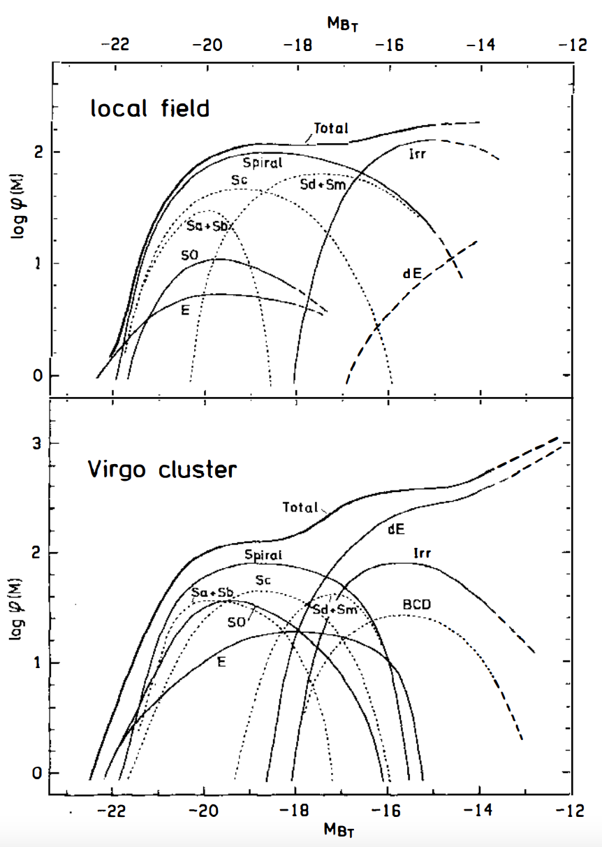
Figure 18.9: Field and cluster galaxy luminosity functions (Binggeli et al. 1988).
This figure shows that the most luminous galaxies are elliptical (“E”) in both clusters and in the field. Spiral galaxies of various types dominate the luminosity function everywhere aside from the most and least luminous ends, with “earlier”-type spiral galaxies (“Sa+Sb” as well as the lenticular galaxies “S0”) being more luminous than later-type spirals (“Sc”, “Sd+Sm”). The least luminous galaxies consist largely of dwarf galaxies (dwarf ellipticals “dE” and blue compact dwarf galaxies “BCD”) and irregular galaxies (“Irr”, like the Large Magellanic Cloud locally; see Section 18.3 below for more discussion on the different galaxy types). These results have held up remarkably well until the present day.
The start of large galaxy redshift surveys in the 1980s ushered in a glorious two decades for the galaxy luminosity function. The availability of large samples of galaxies required a detailed statistical treatment of selection biases in the determination of the luminosity function, with the two most popular methods being the \(1/V_\mathrm{max}\) method of Schmidt (1968) and variations of the stepwise maximum likelihood method of Efstathiou et al. (1988). The \(1/V_\mathrm{max}\) method simply determines \(n(L)\) by counting all galaxies in the sample with weights \(1/V_\mathrm{max}\), where \(V_\mathrm{max}\) is the maximum comoving volume over which each individual galaxy could be detected by the survey. This intuitively corrects for the fact that fainter galaxies are underrepresented in galaxy surveys (because surveys are generally magnitude-limited and faint galaxies can be seen out to much smaller distances for a given magnitude limit). Maximum-likelihood techniques, however, are based on more rigorous statistical methods. The CfA redshift survey as well as other early redshift surveys allowed detailed determinations of the field luminosity function (Efstathiou et al. 1988; Marzke et al. 1994), culminating in definitive determinations of the optical and near-infrared luminosity functions at low redshift using large galaxy samples from the Sloan Digital Sky Survey in the optical (Blanton et al. 2003b; Blanton et al. 2005) and from 2MASS in the near-infrared (Kochanek et al. 2001). The optical measurements are summarized in the top, left panel of Figure 18.10 taken from Blanton & Moustakas (2009).
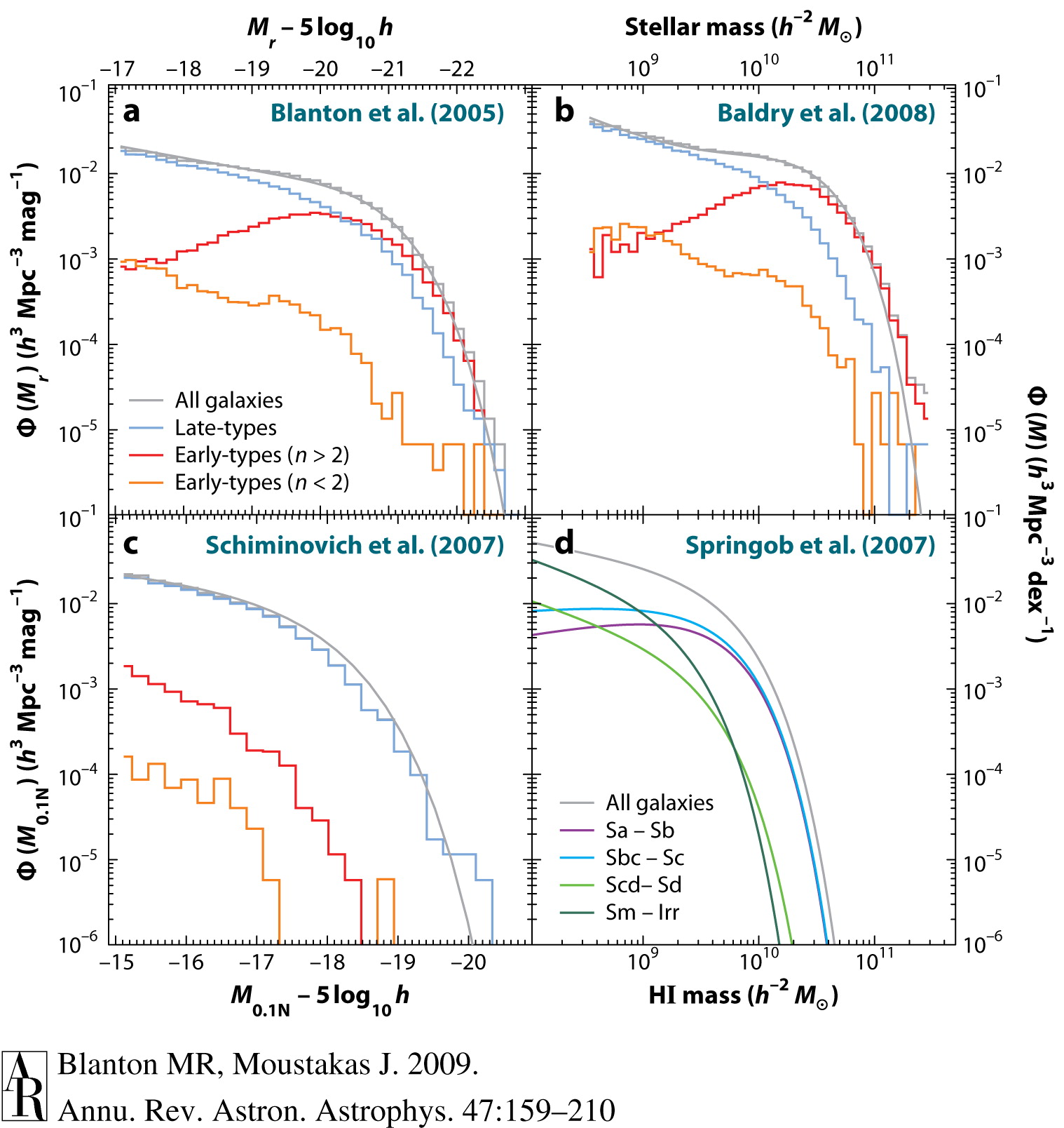
Figure 18.10: Galaxy luminosity and stellar-mass functions (Blanton & Moustakas 2009): low-redshift optical (top, left) and ultraviolet (bottom, left) luminosity functions as well as low-redshift stellar (top, right) and HI (bottom, right) mass functions.
The luminosity function is displayed in this figure as a function \(\Phi(M)\) of absolute magnitude \(M\), which gives the number density in bins of absolute magnitude, rather than of luminosity. This function is related to \(\Phi(L)\) as \begin{equation} \Phi(M) = (0.4\ln 10) \,L\,\Phi(L)\,, \end{equation} because of the relation between luminosity and absolute magnitude. We see that the general luminosity function is characterized by two important behaviors: an increasing \(\Phi(M)\) with increasing \(M\) at larger \(M\), corresponding to low-luminosity galaxies, and a sharply decreasing \(\Phi(M)\) with decreasing \(M\) at smaller \(M\), corresponding to luminous galaxies. The transition between these two regimes is at \(M_r \approx -21\), which is close to the absolute magnitude of the Milky Way (which has a few times \(10^{10}\,L_{r,\odot}\); recall from above that the Sun’s absolute \(r\)-band magnitude is \(4.65\); Willmer 2018). Thus, there are not many galaxies more luminous than the Milky Way, but many galaxies that are far less luminous than the Milky Way exist in the Universe. The increase at low luminosity is dramatic: because \(M \propto \log L\), there is an increasing number of galaxies per decade of luminosity \(L\) with decreasing \(L\); extrapolated to \(L = 0\), there is then an infinite number of low-luminosity galaxies! This divergence, of course, cannot happen in reality and there has to be a transition to a decreasing number of galaxies at some low \(L\) or a low-\(L\) cut-off. But the point is that there is a very large number of low-luminosity galaxies that are, however, difficult to detect.
Galaxy luminosity functions are often summarized using simple parametric forms. The most influential of these is the “Schechter” function, introduced by Schechter (1976) and inspired by the shape of the Press-Schechter formalism’s dark-matter halo mass function discussed in Chapter 17.4. The Schechter function models the high-\(L\) cut-off as an exponential and the fast rise towards low-\(L\) with a power law: \begin{equation}\label{eq-exgal-schechter-L} \Phi(L) = {\Phi^*\over L^*}\,\exp\left(-{L\over L^*}\right)\,\left({L \over L^*}\right)^\alpha\,, \end{equation} where \(\alpha\) is the low-\(L\) logarithmic slope, \(L^*\) is the transition luminosity, and \(\Phi^*\) is the normalization. In terms of the absolute magnitude \(M\), this function becomes \begin{equation} \Phi(M) = (0.4\ln 10) \,\Phi^*\,\exp\left(-10^{0.4\,[M^*-M]}\right)\,10^{0.4\,[\alpha+1]\,[M^*-M]}\,, \end{equation} where \(M^*\) is the absolute magnitude corresponding to \(L^*\). In the optical \(r\) band at \(z \approx 0.1\), we have that \(\Phi^* \approx 0.5\times10^{-2}\,\mathrm{Mpc}^{-3}\), \(M^* \approx -21.2\), and \(\alpha \approx -1.05\) (Blanton et al. 2003b). There is, however, significant uncertainty in the low-\(L\) slope \(\alpha\), mainly because the low-\(L\) tail of the luminosity function is not well represented by a single power law. Instead, a double-Schechter function that has a broken-power law for the low-\(L\) behavior is necessary (Binggeli et al. 1988). This double-Schechter function has the form \begin{equation}\label{eq-exgal-dblschechter-L} \Phi(L) = {1\over L^*}\,\exp\left(-{L\over L^*}\right)\,\left[\Phi^*_1\left({L \over L^*}\right)^{\alpha_1}+\Phi^*_2\left({L \over L^*}\right)^{\alpha_2}\right]\,, \end{equation} where the lowest-\(L\) behavior is characterized by \(\alpha_2 \approx -1.4\). While a double Schechter function typically provides an adequate fit over the full luminosity range probed, the parameters depend on the photometric band and the redshift distribution of the galaxy sample used.
Whereas optical and near-infrared luminosity functions indirectly trace the density of stellar mass in the Universe, luminosity functions in other wavelength ranges probe other properties of the galaxy population. In particular, rest-frame ultraviolet luminosity functions trace the density of star formation at the galaxy population’s redshift and they are, therefore, a way to understand the overall star-formation history of the Universe (see Section 18.5 below). For example, the GALEX space telescope measured the ultraviolet luminosity function at low redshift (\(z\approx 0.1\); Wyder et al. 2005) and at intermediate redshifts (out to \(z \approx 1\); Arnouts et al. 2005) to trace the recent evolution in the Universe’s star formation. The ultraviolet luminosity function at very high redshift (up to \(z \approx 10\) currently) is of great interest to understand early galaxy formation and the effect of young galaxies on the surrounding Universe (e.g., Bouwens et al. 2007; Bouwens et al. 2015). Because dust heated by highly-luminous, massive, young stars radiates in the mid-infrared wavelength region, the mid-infrared luminosity function traces dusty galaxies with high star-formation rates and is, therefore, an alternative way to study star formation at high redshift (e.g., Magnelli et al. 2011).
Using the SDSS \(r\)-band numbers at \(z\approx 0.1\) of \(\Phi^* \approx 0.5\times10^{-2}\,\mathrm{Mpc}^{-3}\) and \(M^* \approx -21.2\) from above, we find that the luminosity density \(j_r\) in the \(r\) band is \(j_r \approx 10^{8}\,L_\odot\,\mathrm{Mpc}^{-3}\). As we saw in Section 18.1.5 above, typical \(r\)-band mass-to-light ratios are \(M/L_r \approx 3\). Using this mass-to-light ratio, we can convert the luminosity density to an estimate of the total stellar-mass density at \(z \approx 0.1\) and we find a few times \(10^{8}\,M_\odot\,\mathrm{Mpc}^{-3}\). Converting this comoving density to a proper density by multiplying by \((1+z)^3\) and dividing the result by the critical density (defined in Equation 17.3), we can then estimate the density parameter of matter contained in stars and stellar remnants and what fraction of the total baryon density parameter this represents:
[35]:
from astropy.cosmology import Planck18
Omega_star= (3*1e8*u.Msun/u.Mpc**3*(1.+0.1)**3
             /Planck18.critical_density(0.1)).to_value(u.dimensionless_unscaled)
print(f"The density parameter of matter contained in galaxies' stars is {Omega_star:.4f}")
print(f"This is {100*Omega_star/Planck18.Ob(0.1):.1f}% of the total baryon density parameter")
The density parameter of matter contained in galaxies' stars is 0.0028
This is 4.8% of the total baryon density parameter
Even using a mass-to-light ratio at the upper limit of what is possible (\(M/L_r \approx 6\)), the fraction of the baryon density would only be \(\approx 10\%\). Thus, baryons contained in stars and stellar remnants constitute only a small fraction of all of the baryons in the present-day Universe. Most of the baryons are in gaseous form in galaxies themselves, in groups and clusters, and in the intergalactic medium between galaxies (e.g., Fukugita et al. 1998; Fukugita & Peebles 2004; de Graaff et al. 2019; Tanimura et al. 2019).
18.2.2. The galaxy stellar mass function
For understanding how galaxies populate dark matter halos, the distribution of the stellar masses of galaxies is more directly relevant than the luminosity function. The stellar mass function \(\Phi(M)\) (somewhat confusingly, ‘\(M\)’ in this context is stellar mass rather than absolute magnitude) is defined similar to the luminosity function of Equation (18.12) as \begin{equation}\label{eq-exgal-smassfunc-def} \Phi(M) = {\mathrm{d} n(M) \over \mathrm{d} M}\,. \end{equation} While we could convert the luminosity function \(\Phi(L)\) to a stellar-mass function using a luminosity-dependent stellar mass-to-light ratio, a more direct path to the stellar mass function is to determine stellar masses for all galaxies in one’s sample using the stellar-population-synthesis (SPS) modeling approach that we discussed in Section 18.1 above and then directly derive the stellar mass function with the same statistical techniques (e.g., \(1/V_\mathrm{max}\) weighting) as used in deriving the luminosity function. Because stellar mass-to-light ratios do not vary that strongly between galaxy types or with color and luminosity, the stellar mass function has a similar shape as the luminosity function and is, in particular, often represented by a Schechter function or a double-Schechter function. Optical and near-infrared bands best trace the total stellar mass in galaxies and, therefore, comprehensive measurements of the stellar mass function at low redshift have been obtained using 2MASS data (e.g., Bell et al. 2003), SDSS data (e.g., Baldry et al. 2008), and other spectroscopic surveys (e.g., Baldry et al. 2012). As a specific measurement example, Baldry et al. (2012) find that the \(z < 0.06\) stellar mass function over the range \(10^8 < M/M_\odot < 10^{11.5}\) is well characterized as a double Schechter function given by \begin{equation}\label{eq-exgal-dblschechter-mass} \Phi(M) = {1\over M^*}\,\exp\left(-{M\over M^*}\right)\,\left[\Phi^*_1\left({M \over M^*}\right)^{\alpha_1}+\Phi^*_2\left({M \over M^*}\right)^{\alpha_2}\right]\,, \end{equation} with \(M^* = 10^{10.66}\,M_\odot \approx 4.6\times 10^{10}\,M_\odot\), \(\Phi^*_1 = 3.96\times 10^{-3}\,\mathrm{Mpc}^{-3}\), \(\alpha_1 = -0.35\), \(\Phi^*_2 = 0.79\times 10^{-3}\,\mathrm{Mpc}^{-3}\), and \(\alpha_2 = -1.47\). As for the luminosity density, the stellar-mass density is given by \(M^*\,\left[\Phi^*_1\,\Gamma(\alpha_1+2) +\Phi^*_2\,\Gamma(\alpha_2+2)\right]\) (see Equation 18.19), which for the low-\(z\) stellar mass function works out to be \(\approx 2.2 \times 10^8\,M_\odot\,\mathrm{Mpc}^{-3}\), agreeing with our estimate based on the luminosity density above.
The determination of stellar masses using SPS modeling has systematic uncertainties due to, e.g., the IMF used, the underlying stellar evolutionary tracks and the spectral library, and stellar population gradients within galaxies that may not be captured by the data or model. Thus, the stellar mass function is more uncertain than the luminosity function.
The top right panel of Figure 18.10 displays the low-\(z\) stellar mass function from Baldry et al. (2008). Comparing the stellar-mass and luminosity functions, we see that (i) the stellar mass function increases more steeply at low masses and (ii) there is a larger difference between the spiral (late types) and elliptical-galaxy (\(n>2\) early types) components of the functions. These differences are both driven by systematic differences in the stellar mass-to-light ratio: elliptical galaxies typically have higher mass-to-light ratios, because they are older, and this combined with their higher luminosity than spirals causes them to stand apart from the spirals at high mass. Stellar mass-to-light ratios also increase towards lower luminosities, so the low-\(L\) end of the luminosity function is compressed into a smaller stellar-mass range, leading to steepening of the low-mass tail.
Using galaxy samples obtained by statistical surveys at higher redshifts, one can determine the redshift evolution of the stellar mass function. This evolution empirically shows the build-up of stellar mass in galaxies during cosmic history. By determining the types of galaxies and the luminosity regime where the biggest changes happen, we can learn where the most important growth of stellar mass occurs. We briefly discuss two examples of determinations of the evolution of the stellar mass function. Moustakas et al. (2013) used data from a novel, efficient spectroscopic survey—PRIMUS (Coil et al. 2011)—to establish the overall evolution of the stellar mass function from \(z \approx 1\) until the present day as well as the evolution of star-forming and quiescent galaxies separately. Galaxies are separated into star-forming and quiescent galaxies using a measurement of their star-formation rate using ultraviolet photometry. Figure 18.11 displays the evolution of the stellar mass function of the star-forming and quiescent galaxy samples.
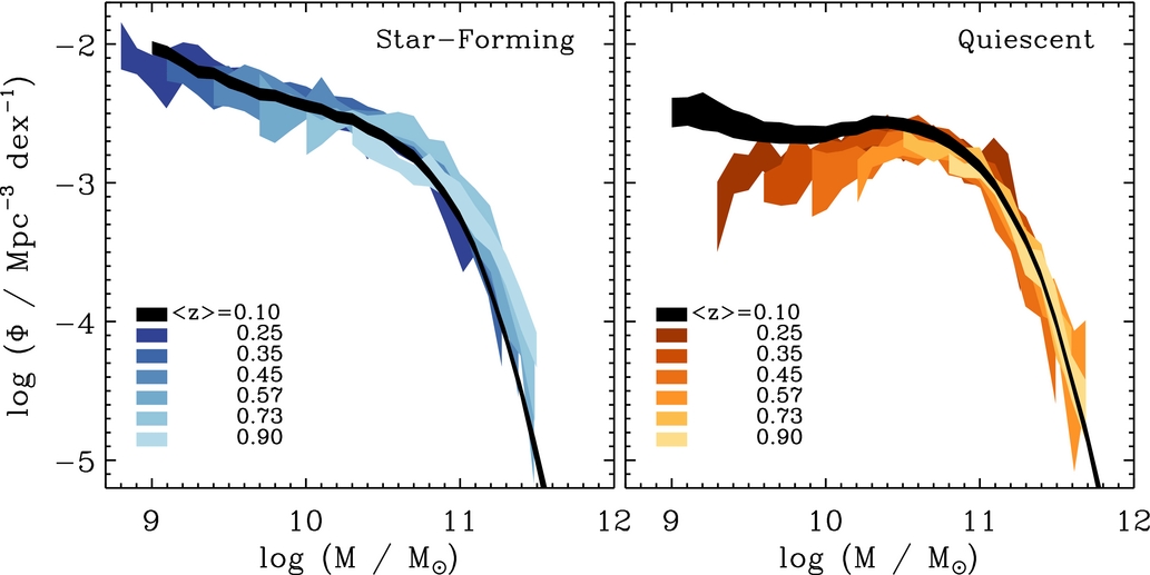
Figure 18.11: Galaxy stellar mass functions up to \(z=1\) (Moustakas et al. 2013).
The first thing to note is that the stellar mass function evolves remarkably little from redshift \(z \approx 1\) (about 8 Gyr ago) until today. Thus, for more than half of cosmic history, the stellar mass function has barely changed (remember that the function is defined in terms of comoving volumes, which removes the decreasing-density evolution from the overall expansion of the Universe). In particular, the low-mass end of the star-forming stellar mass function and the high-mass end of that of the quiescent population does not change. Growth in stellar mass mainly happens at the higher-mass end for star-forming galaxies and at the low-mass end of quiescent galaxies. The high-mass growth in the star-forming population is largely the result of continuous star formation in large spiral galaxies like the Milky Way. The observed growth in stellar mass for the star-forming galaxies is compatible with the growth expected from measurements of the typical star-formation rate of these types of galaxies in this redshift range. Thus, stellar mass in these galaxies mainly builds up through star formation rather than, say, mergers with lower-mass galaxies. The low-mass growth in the quiescent population is driven by low-mass galaxies in the star-forming population ending their star-forming stage and becoming part of the quiescent population in a process known as quenching.
Going to even higher redshifts using photometrically-determined stellar masses, Muzzin et al. (2013) determined the evolution of the stellar mass function out to \(z \approx 4\) as shown in Figure 18.12.
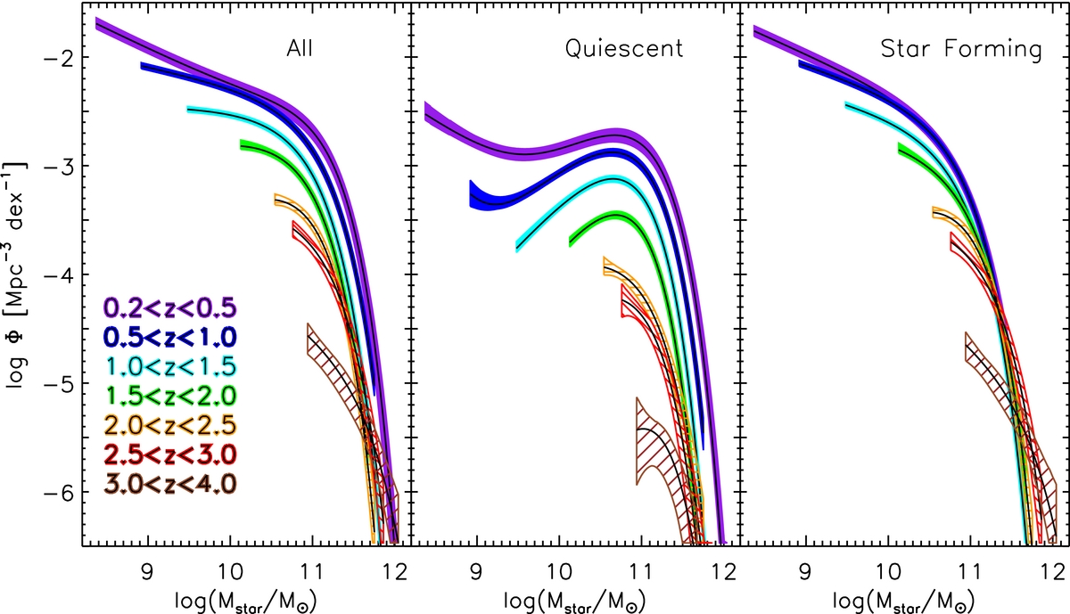
Figure 18.12: Galaxy stellar mass functions up to \(z=4\) (Muzzin et al. 2013).
The \(0 < z < 1\) trends in this figure are largely (but not fully) compatible with those seen by Moustakas et al. (2013), but we now see a more dramatic evolution at \(1 < z < 4\). Ignoring the noisiest, highest-redshift bin, the stellar mass function of all types of galaxies increases strongly between \(z=3.5\) and \(z=1\) and this is in fact the epoch during which galaxies form most of their stars (see Section 18.5 below). Lower-mass galaxies of all types experience stronger growth than massive galaxies.
18.2.3. The stellar-mass–halo-mass relation
While the stellar mass function on its own contains important information about the evolution of the galaxy population over time, galaxies assemble in the dark-matter halos that form through the gravitational collapse of overdense regions of the Universe that grow as the Universe expands (as we discussed in detail in Chapter 17). A fundamental question is therefore: what kind of dark matter halo hosts a galaxy of a given set of properties. These properties could be the galaxy’s stellar mass, its type (spiral, elliptical, or other), its star-formation rate, its environment (in a cluster, in the field, or somewhere in between), etc. As a first step in answering this question, we will focus on the first property: what is the mass of the halo \(M_\mathrm{halo}\) that hosts a galaxy with stellar mass \(M_*\)? Specifically, we seek to determine the ratio \(M_*/M_\mathrm{halo}\) as a function of \(M_\mathrm{halo}\), which is the so-called stellar-mass–halo-mass relation (SMHMR).
A naive estimate of \(M_*/M_\mathrm{halo}\) is that it should simply equal the baryon-to-matter ratio \(\Omega_b/\Omega_m\) (note that this ratio does not depend on redshift, because both of the density parameters have the same redshift evolution). This assumes that halos form from the cosmological mixture of baryons and dark matter (a reasonable assumption) and that all of the initially-gaseous baryons are turned into stars and stellar remnants through star formation. However, by comparing the stellar mass function given above and the halo mass function that we determined using the Press-Schechter formalism in Chapter 17.4, we directly see that this cannot be the case. To demonstrate this, in Figure 18.13, we plot the stellar mass function from above, the halo mass function from Chapter 17.4 (specifically, the more accurate Sheth & Tormen 1999 mass function, which we also use everywhere below), and the halo mass function shifted to masses \(\Omega_b/\Omega_m\) lower, which is the predicted stellar mass function when \(M_*/M_\mathrm{halo}=\Omega_b/\Omega_m\).
[36]:
from astropy.cosmology import Planck18
def stellar_mass_function(M,Mstar=10.**10.66*u.Msun,
                         phi1= 3.96*1e-3/u.Mpc**3,
                         alpha1=-0.35,
                         phi2= 0.79*1e-3/u.Mpc**3,
                         alpha2=-1.47):
    # d Mstellar / d ln M
    return M/Mstar*numpy.exp(-M/Mstar)*(phi1*(M/Mstar)**alpha1
                                        +phi2*(M/Mstar)**alpha2)
sms= numpy.geomspace(1e6,1e12,251)*u.Msun
smf= u.Quantity([stellar_mass_function(m) for m in sms])
figure(figsize=(8,5))
loglog(sms,smf.to_value(1./u.Mpc**3),
       label=r'$\mathrm{Stellar\ mass\ function}$')
################### Halo mass function from Chapter 18 #############
# Constants
Om0= 0.3111
Ode0= 0.6889
H0= 67.70*u.km/u.s/u.Mpc
h= (H0/(100.*u.km/u.s/u.Mpc)).to_value(u.dimensionless_unscaled)
Ob0= 0.0490
ns= 0.9665
As= numpy.exp(3.047)*1e-10
kp= 0.05/u.Mpc
from scipy import integrate
from astropy.constants import c, G
rhom= Om0*3.*H0**2./8./numpy.pi/G
# Transfer function approximation
T0CMB= 2.7255*u.K
def transfer_bbks(k,model='BBKS',Om0=Om0,h=h,Ob0=Ob0,T0CMB=T0CMB):
    if model.lower() == 'bbks':
        q= (k/(Om0*h**2./u.Mpc)).to_value(u.dimensionless_unscaled)
    elif model.lower() == 'sugiyama':
        q= (k*(T0CMB/2.7/u.K)**2./(Om0*h**2./u.Mpc)/numpy.exp(-Ob0-numpy.sqrt(2.*h)*Ob0/Om0))\
        .to_value(u.dimensionless_unscaled)
    return numpy.log(1.+2.34*q)/2.34/q*(1.+3.89*q+(16.1*q)**2.
                                        +(5.46*q)**3.+(6.71*q)**4.)**-0.25
# Growth factor stuff
def H(a):
    # Assumes flat Universe
    return H0*numpy.sqrt(Om0/a**3.+Ode0)
def growth_factor(a):
    return (5.*Om0/2.*H(a)/H0\
        *integrate.quad(lambda ap: 1./ap**3./(H(ap)/H0)**3.,
                        0.,a)[0]).to_value(u.dimensionless_unscaled)
# Matter power spectrum without the growth factor, so we can apply it later
def matter_power_spectrum_nogrowth(k,model='BBKS'):
    return 8.*numpy.pi**2./25.*c**4.*As*kp/Om0**2./H0**4.\
        *transfer_bbks(k,model=model)**2.*(k/kp)**ns
def window(x):
    # Top-hat window function in Fourier space
    return 3.*(numpy.sin(x)-x*numpy.cos(x))/x**3.
def sigma2_R(R,a=1.):
    # sigma2 computed as a function of R at scale factor a
    return integrate.quad(lambda k: k**2.\
        *matter_power_spectrum_nogrowth(k/u.Mpc,
                                        model='Sugiyama').to_value(u.Mpc**3)\
        *window((k*R/u.Mpc).to_value(u.dimensionless_unscaled))**2,
                          0,numpy.inf)[0]/2./numpy.pi**2.*growth_factor(a)**2.
def sigma2(M,a=1.):
    # sigma2 computed as a function of mass M
    R= 1.82*u.Mpc*(M/1e12/u.Msun)**(1./3.)
    return sigma2_R(R,a=a)
def dwindowdx(x):
    return 3.*((3.*x*numpy.cos(x)+(x**2.-3.)*numpy.sin(x))/x**4.)
def dlnsigmadlnM(M):
    # constant with a, so set a=1.
    R= 1.82*u.Mpc*(M/1e12/u.Msun)**(1./3.)
    return integrate.quad(lambda k: k**2.\
        *(k*R/u.Mpc).to_value(u.dimensionless_unscaled)\
        *matter_power_spectrum_nogrowth(k/u.Mpc,
                                        model='Sugiyama').to_value(u.Mpc**3)\
        *window((k*R/u.Mpc).to_value(u.dimensionless_unscaled))\
        *dwindowdx((k*R/u.Mpc).to_value(u.dimensionless_unscaled)),
                          0,numpy.inf)[0]\
        /6./numpy.pi**2.*growth_factor(1.)**2./sigma2_R(R,a=1.)
def halo_mass_function(M,a=1.,model='PS',dlnsigdlnM=None,sig=None):
    # d n / d ln M
    # Use sigma and d ln sigma / d ln M if provided, otherwise compute
    if sig is None:
        sig= numpy.sqrt(sigma2(M,a=a))
    if dlnsigdlnM is None:
        dlnsigdlnM= dlnsigmadlnM(M)
    # f function
    if model.lower() == 'ps':
        def fnu(nu):
            return numpy.sqrt(2./numpy.pi)*nu*numpy.exp(-nu**2./2.)
    elif model.lower() == 'st':
        def fnu(nu):
            nu= numpy.sqrt(0.707)*nu
            return 0.3222*numpy.sqrt(2./numpy.pi)*nu*numpy.exp(-nu**2./2.)\
                *(1.+nu**-0.6)
    nu= 1.686/sig
    return -rhom/M*fnu(nu)*dlnsigdlnM
hms= numpy.geomspace(1e5,1e16,51)*u.Msun
hmf= u.Quantity([halo_mass_function(m,model='st') for m in hms])
loglog(hms,hmf.to_value(1./u.Mpc**3),
       label=r'$\mathrm{Halo\ mass\ function}$')
loglog(hms*Planck18.Ob(0)/Planck18.Om(0),hmf.to_value(1./u.Mpc**3),
       label=r'$\mathrm{Halo\ mass\ function} \leftarrow \Omega_b/\Omega_m$')
xlabel(r'$M/M_\odot$')
ylabel(r'$\mathrm{d} n/\mathrm{d} \ln M\,(\mathrm{Mpc}^{-3})$')
ylim(1e-10,4e4)
legend(frameon=False,fontsize=18.);

Figure 18.13: Observed stellar mass function compared to the Sheth & Tormen (1999) halo mass function. The final curve is the predicted stellar mass function if a galaxy’s stellar mass is the universal baryon fraction times its halo mass.
We see that the shifted halo mass function does not agree at all with the stellar mass function. The shifted halo mass function is above the stellar mass function at all masses, meaning that at no stellar mass do galaxies turn all of their baryons into stars. Thus, star formation in galaxies is inefficient, which is something we already knew from the calculation of the density parameter of matter contained in galaxies’ stars in Section 18.2.1. However, the fact that the shape of the stellar and (shifted) halo mass functions is so different means that the SMHMR must have a strong dependence on halo mass.
Determining the relation between halo mass and stellar mass is difficult, because it is so hard to determine total halo masses. While we can obtain galaxy stellar masses through SPS modeling, determining the total halo mass requires us to measure the mass out to the halo’s virial radius, well beyond the reach of the dynamical tracers that are typically used to determine the mass distributions in galaxies at smaller distances. The only robust way to measure total halo masses currently is through weak gravitational lensing—determining the mass profile of a cluster or galaxy by looking for the subtle changes to the shapes of background galaxies due to the effect of gravitational lensing (see Chapter 15.3.4). However, while weak lensing can be applied to determine the mass of a single galaxy cluster, the number of background sources behind individual galaxies is too small to be able to determine the mass of a single galaxy through weak lensing. Therefore, weak-lensing galaxy halo masses are typically obtained by combining the weak constraints from many individual galaxies. Constraints on the SMHMR from weak lensing have been presented by, e.g., Hoekstra et al. (2005), Mandelbaum et al. (2006), Leauthaud et al. (2012), and van Uitert et al. (2016). We show some of these results in Figure 18.16 below.
A less empirical way to determine the SMHMR is to circumvent the issue of measuring total halo masses by assuming that the halo mass distribution predicted by the cosmological framework is correct and that all we have to do is to assign stellar masses to the dark-matter halos. One popular way of doing this is through abundance matching, which assigns galaxies to dark-matter halos by requiring that galaxies with a given property (e.g., stellar mass) live in dark-matter halos that exist in the same abundance as the galaxy sample in question (Vale & Ostriker 2004). Typically, this abundance matching is done using \(N\)-body simulations of structure formation in the Universe (e.g., Behroozi et al. 2010; Moster et al. 2010b; Guo et al. 2010). Stellar masses drawn from the observed stellar mass function are then assigned to dark matter halos (and subhalos, see below) as follows: in a given volume, the galaxy with the highest stellar mass is assigned to the most massive dark-matter halo, the second-highest stellar mass is assigned to the second-most-massive dark-matter halo, and so on. Here, we present a similar approach following Vale & Ostriker (2004) that directly uses the stellar and halo mass functions to achieve the same result.
To match galaxies and halos by abundance as a function of stellar/halo mass, we require that the cumulative number density \(N^*(>M_*)\) of galaxies matches the cumulative number density \(N^h(>M_\mathrm{halo})\) of halos. At a given matching cumulative number density \(N^*(>M_*)=N^h(>M_\mathrm{halo})\), galaxies with \(M_*\) then live in halos with mass \(M_\mathrm{halo}\). Both of these cumulative number densities are easily computed from the stellar and halo mass functions. But before doing so, we need to deal with a subtlety about the halo mass function as computed using the Press-Schechter formalism in Chapter 17.4, namely that that halo mass function does not take subhalos—halos contained within and gravitationally-bound to another larger halo—into account, while such subhalos also host galaxies (those are satellite galaxies, like the Large Magellanic Cloud in the Milky Way, and they are included in the stellar mass function). To take subhalos into account, we can use the fact that the distribution of subhalos is approximately self-similar in the \(\Lambda\)CDM Universe that we live in (Springel et al. 2008a), so the number of subhalos \(n_{\mathrm{sh}}(m|M)\) of a given mass \(m\) inside a larger halo of mass \(M\) can be approximated by a function that only depends on \(m/M\). In particular, we use the expression from Vale & Ostriker (2004): \begin{equation} {\mathrm{d} n_{\mathrm{sh}}(m|M) \over \mathrm{d} \ln m} = {\gamma \over \beta\, \Gamma(2-\alpha)}\,\left({m\over x\beta M}\right)^{-\alpha}\,\exp\left(-{m\over x\beta M}\right)\,, \end{equation} where \(\alpha = 1.91\), \(\beta = 0.39\), \(\gamma = 0.18\), \(x=3\), and \(\Gamma(\cdot)\) is the gamma function (see Appendix B.3.3). The halo mass function that includes subhalos is then obtained by convolving the halo mass function \(\mathrm{d} n_{\mathrm{mh}} / \mathrm{d} \ln M\) for main halos with the subhalo distribution, which gives the total abundance of subhalos, and adding the main-halo mass function \begin{equation} {\mathrm{d} n_{\mathrm{mh+sh}}(M) \over \mathrm{d} \ln M} = {\mathrm{d} n_{\mathrm{mh}}(M) \over \mathrm{d} \ln M } + \int_0^\infty \mathrm{d} \ln \tilde{M} {\mathrm{d} n_{\mathrm{sh}}(M|\tilde{M}) \over \mathrm{d} \ln M}\,{\mathrm{d} n_{\mathrm{mh}}(\tilde{M}) \over \mathrm{d} \ln \tilde{M}}\,. \end{equation}
The following code computes the main-halo+subhalo mass function and compares it to the main-halo mass function:
[37]:
from scipy import special, interpolate, integrate
def interp_mf(masses,mfs):
    return interpolate.InterpolatedUnivariateSpline(numpy.log(masses.to_value(u.Msun)),
                                                    numpy.log(mfs.to_value(1./u.Mpc**3)))

hmf_ipl= interp_mf(hms,hmf)
def dnsubdlnm(subhalo_mass,parent_mass):
    _ALPHA= 1.91
    _BETA= 0.39
    _GAMMA= 0.18
    amp= _GAMMA/_BETA/special.gamma(2.-_ALPHA)
    _X= 3.
    reduced_mass= subhalo_mass/_X/_BETA/parent_mass
    return amp*reduced_mass**-_ALPHA\
        *numpy.exp(-reduced_mass)*reduced_mass
def hmf_total(mass,hmf_ipl):
    return (integrate.quad(lambda lnparent_mass: dnsubdlnm(mass,numpy.exp(lnparent_mass)*u.Msun)*numpy.exp(hmf_ipl(lnparent_mass)),
                          numpy.log(numpy.amin(hms.to_value(u.Msun))),
                          numpy.log(numpy.amax(hms.to_value(u.Msun))))[0]\
        +numpy.exp(hmf_ipl(numpy.log(mass.to_value(u.Msun)))))/u.Mpc**3
figure(figsize=(8,5))
loglog(hms,hmf.to_value(1./u.Mpc**3),
       label=r'$\mathrm{Halo\ mass\ function}$')
hshmf= u.Quantity([hmf_total(hm,hmf_ipl) for hm in hms])
loglog(hms,hshmf.to_value(1./u.Mpc**3),
       label=r'$\mathrm{Halo+subhalo\ mass\ function}$')
xlabel(r'$M/M_\odot$')
ylabel(r'$\mathrm{d} n/\mathrm{d} \ln M\,(\mathrm{Mpc}^{-3})$')
ylim(1e-10,4e4)
legend(frameon=False,fontsize=18.);

Figure 18.14: The halo mass function including subhalos.
We see that the two mass functions coincide at high masses, where subhalos are rare, but at low masses, the large number of subhalos in high-mass halos creates a significant increase in the abundance of halos. From now on, we will include subhalos whenever we say “halo mass function” below.
We are now ready to start abundance matching galaxies and halos. As a first step, we compute the cumulative number densities of galaxies and halos as a function of stellar and halo mass, respectively. We also store an interpolated version of the inverse cumulative number density functions to perform the \(N^*(>M_*)=N^h(>M_\mathrm{halo})\) abundance matching below. To illustrate the abundance-matching process, we indicate how the stellar and halo mass functions are matched by abundance for a few values of the stellar/halo mass in Figure 18.15.
[38]:
smf_ipl= interp_mf(sms,smf)
hmf_ipl= interp_mf(hms,hshmf)
def cumul_mf(masses,mf_ipl):
    return numpy.array(\
            [integrate.quad(lambda x: numpy.exp(mf_ipl(x)),
                            numpy.log(mass.to_value(u.Msun)),
                            numpy.log(numpy.amax(masses.to_value(u.Msun))))[0]
             for mass in masses[:-2]])
def interp_invcumul_mf(masses,mf_ipl):
    return interpolate.InterpolatedUnivariateSpline(\
                numpy.log10(cumul_mf(masses,mf_ipl)[::-1]),
                numpy.log10(masses[:-2][::-1].to_value(u.Msun)))
icsmf_ipl= interp_invcumul_mf(sms,smf_ipl)
ichmf_ipl= interp_invcumul_mf(hms,hmf_ipl)
figure(figsize=(8,5))
loglog(sms[:-2],cumul_mf(sms,smf_ipl),
       label=r'$\mathrm{Stellar\ mass\ function}$')
loglog(hms[:-2],cumul_mf(hms,hmf_ipl),
       label=r'$\mathrm{Halo\ mass\ function}$')
xlabel(r'$M/M_\odot$')
ylabel(r'$N(>M)\,(\mathrm{Mpc}^{-3})$')
l10densities= [numpy.log10(2e-1),-3,-7]
for l10density in l10densities:
    annotate('',xy=(10.**ichmf_ipl(l10density),10.**l10density),
             xytext=(10.**icsmf_ipl(l10density),10.**l10density),
             arrowprops=dict(facecolor='k',width=1.,shrink=0.))
legend(frameon=False,fontsize=18.);

Figure 18.15: Abundance matching.
Using the inverse cumulative number density functions, we can then require \(N^*(>M_*)=N^h(>M_\mathrm{halo})\) and derive \(M_*\) as a function of \(M_\mathrm{halo}\). For \(M_\mathrm{halo}\), the cumulative number density is \(\nu = N^h(>M_\mathrm{halo})\), corresponding to \(M_* = (N^*)^{-1}(\nu)\). The resulting SMHMR is then shown as the thick curve in Figure 18.16. As discussed above, \(M_*/M_\mathrm{halo}\) does not reach the universal baryon fraction \(\Omega_b/\Omega_m\) at any halo mass. The maximum \(M_*/M_\mathrm{halo}\) is \(\approx 0.03 \ll \Omega_b/\Omega_m \approx 0.16\) at \(M_\mathrm{halo} \approx 10^{12}\,M_\odot\), approximately the mass of the Milky Way. Thus, galaxy halos like the Milky Way’s are the most efficient at turning baryons into stars, but their efficiency is nevertheless low at \(\approx 20\%\). At higher and lower halo masses, star formation in galaxies is far less efficient still and the ratio \(M_*/M_\mathrm{halo}\) drops precipitously towards higher and lower halo masses. The reason for this low star-formation efficiency in galaxies is an important, ongoing problem in galaxy evolution, but it is believed to be caused by various feedback processes, such as energy and momentum injection into star-forming gas by stellar winds, supernova explosions, and winds driven by active galactic nuclei (see Chapter 19.3.3). This injection makes it harder for gas to cool and form stars and it can expel gas entirely from galaxies into the intergalactic medium. Supernova explosions and stellar winds have their largest effect at the low-mass end (\(M_\mathrm{halo} \lesssim 10^{12}\,M_\odot\)), while active galactic nuclei are mostly important at higher masses (\(M_\mathrm{halo} \gtrsim 10^{12}\,M_\odot\)).
While our implementation of abundance matching is simple, it compares well to both direct measurements from lensing (Hoekstra et al. 2005; Mandelbaum et al. 2006; Leauthaud et al. 2012) and to more sophisticated, \(N\)-body-based abundance matching (Behroozi et al. 2010; Moster et al. 2010b) as shown in Figure 18.16. First, we write some code to download and read the literature measurements from a compilation maintained by Alexie Leauthaud:
[39]:
import sys
import os
from pathlib import Path
import shutil
import subprocess
import tempfile
from astropy.io import ascii
_MAX_DOWNLOAD_NTRIES= 2
_ERASESTR= "                                                                                "
_CACHE_BASEDIR= Path(os.getenv('HOME')) / '.galaxiesbook' / 'cache'
_CACHE_SMHMR_DIR= _CACHE_BASEDIR / 'smhmr'
_SMHMR_URL= 'https://galaxiesbook.org/data/shmr_archive.tar'
def read_smhmr_compilation(identifier):
    archive_filePath= _CACHE_SMHMR_DIR / 'shmr_archive.tar'
    _download_smhmr_compilation(archive_filePath)
    paths_dict= {
        'hoekstra': 'hoekstra_shmr_compilation_by_AL_2011.txt',
        'mandelbaum': 'mandelbaum_shmr_compilation_by_AL_2011.txt',
        'leauthaud': 'cosmos_2011_mstellar_m200b_0.22_0.48.txt',
        'moster': 'moster_shmr_compilation_by_AL_2011.txt',
        'behroozi': 'behroozi_shmr_compilation_by_AL_2011.txt'
    }
    filePath= _CACHE_SMHMR_DIR / paths_dict[identifier]
    out= ascii.read(filePath)
    out.rename_column('col1','l10m200')
    out.rename_column('col2','l10mstellar')
    return out
def _download_smhmr_compilation(filePath,verbose=False):
    if not Path(filePath).exists():
        _download_file(_SMHMR_URL,filePath,verbose=verbose)
        # Untar
        cmd= ['tar','-xf',filePath,
             '-C',Path(filePath).parent]
        try:
            subprocess.check_call(cmd)
        except subprocess.CalledProcessError as e:
            raise RuntimeError(f"Untarring {filePath} failed")
    return None
def _download_file(downloadPath,filePath,verbose=False,spider=False):
    sys.stdout.write('\r'+"Downloading file %s ...\r" \
                         % (Path(filePath).name))
    sys.stdout.flush()
    try:
        # make all intermediate directories
        os.makedirs(Path(filePath).parent)
    except OSError: pass
    # Safe way of downloading
    downloading= True
    interrupted= False
    file, tmp_savefilename= tempfile.mkstemp()
    os.close(file) #Easier this way
    ntries= 1
    while downloading:
        try:
            cmd= ['curl','-L',downloadPath,
                  '-o',tmp_savefilename,
                  '--fail','--silent','--show-error',
                  '--connect-timeout','10',
                  '--retry','3']
            if not verbose: cmd.append('--silent')
            subprocess.check_call(cmd)
            shutil.move(tmp_savefilename,filePath)
            downloading= False
            if interrupted:
                raise KeyboardInterrupt
        except subprocess.CalledProcessError as e:
            if not downloading: #Assume KeyboardInterrupt
                raise
            elif ntries > _MAX_NTRIES:
                raise IOError('File %s does not appear to exist on the server ...' % (Path(filePath).name))
            elif not 'exit status 4' in str(e):
                interrupted= True
            os.remove(tmp_savefilename)
        finally:
            if Path(tmp_savefilename).exists():
                os.remove(tmp_savefilename)
        ntries+= 1
    sys.stdout.write('\r'+_ERASESTR+'\r')
    sys.stdout.flush()
    return None
and then we plot the literature SMHMR determinations to compare to our own:
[40]:
hoekstra_smhmr= read_smhmr_compilation('hoekstra')
mandelbaum_smhmr= read_smhmr_compilation('mandelbaum')
cosmos_smhmr= read_smhmr_compilation('leauthaud')
behroozi10_smhmr= read_smhmr_compilation('behroozi')
moster_smhmr= read_smhmr_compilation('moster')
figure(figsize=(9,6))
l10densities= numpy.linspace(-8,numpy.log10(3e-1),101)
p= loglog(10.**ichmf_ipl(l10densities)*u.Msun,
          10.**(icsmf_ipl(l10densities)-ichmf_ipl(l10densities)),
          lw=3.,zorder=-10,
          label=r'$\texttt{galaxiesbook.org}$')
def l10smhm_approx(l10hm):
    out= numpy.zeros_like(l10hm)
    out= numpy.polyval([0.0809064363713381,-0.3326332856217131,0.2398618485447382,
                        0.1316612250966421,0.2195760607130827,0.5915199066285778,
                        0.6235489869631337,0.0228248361508645,-38.8653378549064428,
                        97.1363140276930039,-84.8790778105431514,22.2879429748974509],
                       (15.-l10hm)**0.54)
    indx= l10hm < 11.
    out[indx]= 1.05*l10hm[indx]-14.05
    indx= l10hm > 13.5
    out[indx]= -0.75*l10hm[indx]+7.85
    return out
loglog(10.**ichmf_ipl(l10densities)*u.Msun,
       10.**l10smhm_approx(ichmf_ipl(l10densities)),zorder=-100,
       color=p[-1].get_color(),ls='--')
plot(10.**mandelbaum_smhmr['l10m200'][1:],
     10.**(mandelbaum_smhmr['l10mstellar']-mandelbaum_smhmr['l10m200'])[1:],'o',
    label=r'$\mathrm{Mandelbaum\ et\ al.\ (2006)}$')
plot(10.**hoekstra_smhmr['l10m200'],
     10.**(hoekstra_smhmr['l10mstellar']-hoekstra_smhmr['l10m200']),'o',
    label=r'$\mathrm{Hoekstra\ et\ al.\ (2007)}$')
plot(10.**cosmos_smhmr['l10m200'],
     10.**(cosmos_smhmr['l10mstellar']-cosmos_smhmr['l10m200']),
     '-',
    label=r'$\mathrm{Leauthaud\ et\ al.\ (2012)}$')
plot(10.**behroozi10_smhmr['l10m200'],
     10.**(behroozi10_smhmr['l10mstellar']-behroozi10_smhmr['l10m200']),
     '--',
    label=r'$\mathrm{Behroozi\ et\ al.\ (2010)}$')
plot(10.**moster_smhmr['l10m200'],
     10.**(moster_smhmr['l10mstellar']-moster_smhmr['l10m200']),
     '--',
    label=r'$\mathrm{Moster\ et\ al.\ (2010)}$')
xlabel(r'$M_{\mathrm{halo}}/M_\odot$')
ylabel(r'$M_*/M_{\mathrm{halo}}$')
xlim(1e10,1e16)
ylim(0.0001,0.5)
gca().yaxis.set_major_formatter(FuncFormatter(
                lambda y,pos: (r'${{:.{:1d}f}}$'.format(int(\
                    numpy.maximum(-numpy.log10(y),0)))).format(y)))
axhline(Planck18.Ob(0)/Planck18.Om(0),color='k',lw=2.)
text(1e14,0.225,r'$\Omega_b/\Omega_m$',size=19.)
legend(frameon=False,fontsize=16.,loc=(0.18,0.));

Figure 18.16: The SMHMR from abundance matching compared to direct observations of the SMHMR and to popular models of the SMHMR (dashed).
The shape of the SMHMR does not lend itself well to a simple functional description, but the following somewhat contrived form matches the form we derived well: \begin{equation}\label{eq-exgal-smhmr} \log_{10} \left({M_*\over M_{\mathrm{halo}}}\right) = \begin{cases} \phantom{-}1.05\,\mu-14.05 & \phantom{11 \leq }\ \mu < 11\\ \phantom{-}\mathrm{see\ below} & 11 \leq \mu \leq 13.5\\ -0.75\,\mu+7.85 & \phantom{11 \leq }\ \mu > 13.5\end{cases}\,,\quad \mathrm{where}\ \mu = \log_{10}\left(M_{\mathrm{halo}}/M_\odot\right)\,, \end{equation} and the \(11 \leq \mu \leq 13.5\) behavior is given by \begin{align} \log_{10} \left({M_*\over M_{\mathrm{halo}}}\right) = & \ 0.0809064363713381\, x^{11} - 0.332633285621713\, x^{10} \nonumber\\ & + 0.239861848544738\, x^{9} + 0.131661225096642\, x^{8} \nonumber\\&+ 0.219576060713083\, x^{7} + 0.591519906628578\, x^{6} \\& + 0.623548986963134\, x^{5} + 0.0228248361508645\, x^{4} \nonumber\\& - 38.8653378549064\, x^{3} + 97.136314027693\, x^{2}\nonumber\\& - 84.8790778105432\, x + 22.2879429748975\nonumber\,, \end{align} where \begin{equation} x = \left[15-\mu\right]^{0.54} = \left[15-\log_{10}\left(M_{\mathrm{halo}}/M_\odot\right)\right]^{0.54}\,. \end{equation} This approximation is displayed as a dashed line in Figure 18.16, but it is so good that it can barely be discerned. The approximate form makes it clear that \begin{equation}\label{eq-exgal-smhmr-lowmass} M_* \propto M_{\mathrm{halo}}^2\,,\quad M \lesssim 10^{12}\,M_\odot\,, \end{equation} and \begin{equation}\label{eq-exgal-smhmr-highmass} M_* \propto M_{\mathrm{halo}}^{0.25}\,,\quad M \gtrsim 10^{12}\,M_\odot\,. \end{equation} Massive galaxies and clusters therefore almost have the same stellar mass regardless of their halo mass. Matching the amplitude and detailed shape of the SMHMR is an important open problem in ab-initio galaxy formation models.

 .
. .
. .
.