
17. Mass modeling in elliptical galaxies
To conclude this third part of the book, we apply what we have learned so far and particularly in this part, to investigate the mass distribution within elliptical galaxies. While they may at first glance look less interesting than spiral galaxies, we’ll see that the internal mass and orbital distribution of elliptical galaxies is actually quite interesting and that much can be learned about the formation and evolution of galaxies and their constituents by dissecting the internal structure of elliptical galaxies. Our approach will be to zoom out from the center to the far reaches of the dark matter halo, starting with a discussion of the dynamics and mass distribution within the inner few hundred parsec and continuing with the internal orbital structure of the stellar component of different types of elliptical galaxies, before ending with the distribution of dark matter out to hundreds of kiloparsec. On this journey, we will need the full complement of axisymmetric and triaxial dynamical modeling combined with the different regimes of gravitational lensing to fully comprehend the structure of elliptical galaxies.
17.1. Supermassive black holes at the centers of galaxies
One of the great discoveries of the second half of the 1990s (aside from cosmic acceleration) is the fact that every massive galaxy has a supermassive black hole at its center. This field developed extraordinarily quickly, going from tentative evidence to full acceptance and statistical studies in just five years. Kormendy & Richstone (1995) summarized the tentative detections of eight supermassive black holes in 1995: starting with the first observations and a simple analysis using spherical and isotropic models of a central black hole in M87 (Sargent et al. 1978; Young et al. 1978; eventually confirmed with gas kinematics by Harms et al. 1994), the field had slowly developed over almost twenty years to eight tentative detections. Six of these were made by dynamical modeling of stellar kinematics, while two came from the more complex modeling of gas kinematics. By using two-integral axisymmetric modeling and three-integral Schwarzschild modeling (e.g., Magorrian et al. 1998; van der Marel et al. 1998; Cretton & van den Bosch 1999; Gebhardt et al. 2003) of observations using the Hubble Space Telescope (HST), evidence for central mass concentrations became highly secure by the year 2000 (we’ll refer to these as supermassive black holes, for some reason usually abbreviated as SMBHs). HST observations were crucial for this: the increased spatial resolution that was possible with HST was necessary to properly resolve the inner dynamical structure and rule out less dense central mass concentrations. This allowed for the demographics of the SMBH population as well as correlations between the SMBH mass and galaxy properties to be determined (e.g., Ferrarese & Merritt 2000; Gebhardt et al. 2000a). The connection between SMBHs and their galaxy has proven to be fertile ground for studying galaxy evolution that continues into the present day. In this section, we briefly discuss the dynamical evidence for SMBHs obtained using the dynamical-modeling techniques that we discussed in parts two and three.
The presence of SMBHs at the centers of a galaxies can be detected with a large variety of techniques. In the low-redshift Universe, these are mainly (i) spectroscopic and astrometric observations of the stars near the Milky Way’s SMBH (see below), (ii) water megamasers (e.g., Miyoshi et al. 1995), (iii) gas kinematics traced using emission-line kinematics (e.g., Harms et al. 1994), and (iv) stellar kinematics combining photometry and absorption-line kinematics. For SMBHs that are ‘active’, that is, that accrete matter at a high enough rate to show up as active galactic nuclei or quasars, other techniques such as the properties of the fluorescent Fe K\(\alpha\) line (Reynolds & Nowak 2003) and reverberation mapping (Blandford & McKee 1982) are possible. We’ll focus here on the evidence coming from stellar kinematics, because it was crucial in establishing the presence of SMBHs in galaxies. Gas kinematics, while a powerful method, suffers from the issue that gas responds to non-gravitational forces that are difficult to capture in models (although we should note that this does not appear to be a concern in galaxies with a Keplerian nuclear gas and dust disk, which provide some of the best SMBH masses; e.g., Ferrarese et al. 1996). Megamasers—gas clouds orbiting very close to the SMBH that act as masers (Lo 2005)—are relatively rare, so while they provide some of the most precise SMBH masses, they cannot easily probe the population of SMBHs. Similarly, the SMBH in our own Milky Way can be studied in exquisite detail, but it is just one SMBH. Stellar kinematics, however, can be used to investigate SMBHs in any massive elliptical galaxy. Of course, the fact that all different methods pointed towards the same population of SMBHs in galaxies was an important part of the acceptance of the SMBH population.
As we will see below, a central SMBH has \(\ll 1\%\) of the mass of a galaxy, so its effect on the orbits of stars and gas is limited to those very close to the SMBH. Because the centers of galaxies have quite well defined velocity dispersions \(\sigma\) that are relatively constant out to radii far larger than where the SMBH affects orbits, the velocity dispersion \(\sigma\) reflects the galactic potential rather than the SMBH potential. Because an SMBH gives rise to a Keplerian rotation curve with its characteristic \(v_c^2 \propto 1/r\) behavior (Equation 3.40), a typical radius \(r_h\) within which the SMBH must dominate the gravitational potential is that where the Keplerian rotation velocity equals the velocity dispersion. Thus, for an SMBH with mass \(M_\bullet\) (Peebles 1972)
or in angular units for a galaxy at a distance \(D\)
The volume within this radius is known as the sphere of influence. Thus, to resolve the sphere of influence for galaxies in the Local Universe, we need to resolve the inner tens of parsec, or equivalently, angular scales well below an arcsecond. Resolving such small angular scales from the ground requires adaptive optics even at the best astronomical sites, because the effect of atmospheric blurring (“seeing”) at even the best astronomical sites is \(\gtrsim 0.5''\). This demonstrates why the Hubble Space Telescope was such a game changer: with its 2.4m diameter mirror in space unencumbered by the atmosphere, the diffraction limit in the optical is \(\approx 0.05''\), allowing the sphere of influence of SMBHs in the Local Universe to be resolved.
Before discussing the application of stellar dynamical modeling to SMBH detection, we need to establish that the methods that we have used for galaxies so far are applicable in this context. Aside from that of equilibrium, there are two fundamental assumptions that need to hold for the application of the techniques discussed in Chapter 6, Chapter 11, and Chapter 15: (i) that the gravitational potential and the stellar motions are non-relativistic and thus described by Newtonian mechanics, and (ii) that the system is collisionless and therefore described by the collisionless Boltzman equation (6.30). The non-relativistic assumption is a priori suspect, because a black hole lives in the regime where the general theory of relativity (GR) is required and where motions become relativistic (that is, speeds are close to the speed of light). Even though black holes don’t have hard surfaces, their typical radius is the Schwarzschild radius
which is the radius where time-dilation becomes infinite in GR and which can be computed in Newtonian gravity as the radius where the escape velocity equals the speed of light. Technically, Equation \eqref{eq-ellipmass-schwarzschild} is the limiting radius only for a non-rotating black hole, but for rotating (Kerr) black holes, the Schwarzschild radius is about the same. Far outside the Schwarzschild radius, the GR black-hole metric closely approaches the Newtonian gravitational potential of a point mass and motions are non-relativistic. Putting in the numbers, for a solar-mass black hole, the Schwarzschild radius is 3 km. Comparing Equation \eqref{eq-ellipmass-sphere-influence} to Equation \eqref{eq-ellipmass-schwarzschild}, we see that
and, thus, \(r_h/r_\bullet \gtrsim 10^6\) for typical massive-galaxy velocity dispersions. Galaxy kinematics around or just inside the sphere of influence is therefore solidly in the non-relativistic regime where we can use Newtonian gravity. This practical advantage is, however, also a significant drawback in the quest for finding SMBHs: while we can establish the presence of dense mass concentrations at the centers of galaxies using observed galaxy kinematics, we cannot unambiguously detect the relativistic velocities and other GR effects that would strongly make the case that the dense mass concentrations are actual black holes and not some other dense system. We’ll come back to this below.
Next, we need to establish whether or not the region within the sphere of influence is collisionless. Because the stellar distribution is approximately spherical, we can compute the relaxation time using Equation (6.12) from Chapter 6.1. For this we need the number of gravitating bodies and the dynamical time. To determine both, we need the mass within the sphere of influence. This we can estimate using the virial theorem. For example, approximating the stellar density as constant within the sphere of influence, the scalar virial theorem gives \(M_h = 5\sigma^2 r_h/(3G) \approx 5\times 10^7\,M_\odot\) for \(\sigma = 200\,\mathrm{km\,s}^{-1}\) and \(r_h = 10\,\mathrm{pc}\). This is similar to the mass of the SMBH, \(M_h \approx M_\bullet\), which of course makes sense because the radius of the sphere of influence is where the gravitational effect of the SMBH is similar to that from the stars. Assigning half of this mass to stars, we have that \(N \approx M_\bullet/M_\odot\), because the typical mass of star is \(\approx 0.5\,M_\odot\). The dynamical time is \(t_\mathrm{dyn} \approx r_h / \sigma \approx 5\times 10^4\,\mathrm{yr}\) for \(\sigma = 200\,\mathrm{km\,s}^{-1}\) and \(r_h = 10\,\mathrm{pc}\). Working through all dependencies, we then have that the relaxation time is
Below, we will see that empirically \(M_\bullet \approx \sigma^4\), such that \(t_\mathrm{relax} \propto M_\bullet^{1.25}\). Thus, as long as \(M_\bullet \gtrsim 10^6\,M_\odot\), the kinematics of stars just inside the sphere of influence has a relaxation time of the order of the age of the Universe or longer and the system therefore behaves as an approximately collisionless system. Even though this relaxation time is much smaller than the one for galaxies as a whole that we discussed in Chapter 6.1, crucially \(t_\mathrm{relax} / t_\mathrm{dyn} \approx M_\bullet/(10\,M_\odot) \gg 1\), so even if the system evolves collisionally on very long time scales, on timescales \(\approx 100\,t_{\mathrm{dyn}}\) on which we typically perform dynamical modeling, the system is effectively collisionless.
Dynamical modeling of galaxy centers with black holes can be done using axisymmetric models, because the SMBH acts as a strong central deflector that disrupts the box orbits that would be necessary to support the triaxiality of the mass distribution. We discussed this process in detail for cuspy mass distributions in Chapter 14.4.2, but as we mentioned there, the disruption of box orbits by dense central-mass concentrations like SMBHs is similar. SMBHs with realistic masses relative to the galaxy leave the larger-scale triaxiality of the galaxy intact, while they axisymmetrize the orbital distribution within the sphere of influence (e.g., Gerhard & Binney 1985; Poon & Merritt 2001; Holley-Bockelmann et al. 2002). Therefore, we can use axisymmetric dynamical modeling for the purpose of detecting and constraining SMBHs. Following the Jeans theorem, steady-state axisymmetric models have to be a function of integrals of the motion, either using the two integrals \(E\) and \(L_z\), or three integrals including also the third integral \(I_3\) (the tensor virial theorem demonstrates why a steady-state axisymmetric model cannot be built from a \(f(E)\) distribution function: such a system has to be spherical). In Chapter 11, we were unable to use \(f(E,L_z)\) models for galactic disks, because they inevitably have \(\sigma_R = \sigma_z\) in contradiction with observations in the solar neighborhood. But for galactic centers, they are viable models, because we cannot directly measure \(\sigma_R/\sigma_z\). Because for realistic galactic potentials, there is no easy way to compute the third integral \(I_3\), constructing \(f(E,L_z,I_3)\) models is done using Schwarzschild modeling.
The \(f(E,L_z)\) models are much easier to work with, because they are the analog of the ergodic, spherical \(f(E)\) models in a crucial sense. As we discussed in Chapter 6.6.1, there is a unique \(f(E)\) distribution function that generates a given density \(\rho(r)\) in a spherical potential \(\Phi(r)\). The situation is almost the same for axisymmetric densities \(\rho(R,z)\) generated by an \(f(E,L_z)\) model in an axisymmetric potential \(\Phi(R,z)\), except that the density \(\rho(R,z)\) now uniquely determines the part of the \(f(E,L_z)\) model that is even in \(L_z\), while leaving the odd part of \(f(E,L_z)\) unconstrained (Lynden-Bell 1962; Dejonghe 1986). This makes physical sense, because the density does not care whether an orbit orbits in the clockwise or counterclockwise direction around the \(z\) axis. To determine the odd part of \(f(E,L_z)\), we therefore have to provide additional information, such as the average rotation velocity \(\overline{v_\phi}(R,z)\). More generally, the density directly determines any even moment of an \(f(E,L_z)\) distribution function, while quantities such as the average rotation velocity \(\overline{v_\phi}(R,z)\) determine all odd moments. In particular, the second moments of the distribution function are directly determined by the density. Because the available data can be cast as moments of the distribution function, we can then directly compute the model prediction using the Jeans equations rather than calculating the full \(f(E,L_z)\) model, using Equations (11.8) and (11.9) with \(\overline{v_R^2} = \overline{v_z^2}\) and \(\overline{v_R\,v_z} =0\). Two-integral modeling of galactic centers then proceeds as follows (cf. Chapter 15.3.3) :
Deproject the observed surface brightness for an assumed inclination angle to obtain a three-dimensional model of the luminosity density;
Create a full mass model by converting the luminosity density to a mass density for an assumed mass-to-light ratio and add an SMBH with mass \(M_\bullet\). The dark-matter halo is generally so sub-dominant on these scales that it does not contribute significantly to the enclosed mass and is therefore not included;
Compute the second moments of the distribution function using the Jeans equations and project them onto the line of sight for comparison to the second moment of the observed line-of-sight velocity distribution.
Repeat for different values of the inclination, mass-to-light ratio, and SMBH mass to find the best fit and its uncertainties.
Magorrian et al. (1998) applied two-integral modeling to 36 galaxies with HST photometry, but still using ground-based kinematic data. The ground-based kinematics data are reported as line-of-sight mean velocity \(V\) and dispersion \(\sigma\) obtained by fitting Gaussian models to the line-of-sight velocity distribution. As such, they don’t allow the actual second moment of the line-of-sight velocity distribution to be computed, but the quantity \(\sqrt{V^2+\sigma^2}\) is approximately equal to the second moment in realistic models and this is the quantity used in the modeling. The following figure from Magorrian et al. (1998) displays model fits with and without an SMBH for some of the galaxies in the sample; the inner velocity dispersion provides clear evidence of the presence of an SMBH.
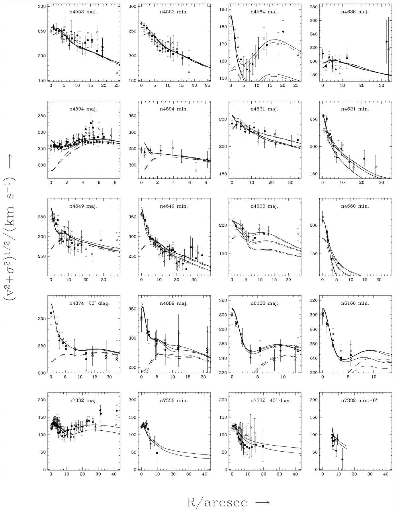
(Credit: Magorrian et al. 1998: Velocity second moment \(\sqrt{V^2+\sigma^2}\) versus distance from the center for illustrative galaxies. The solid curves are for the best-fit model with SMBH, the dashed curves for that without SMBH; different curves with the same linestyle are for different galaxy inclinations)
As we will discuss further below, Magorrian et al. (1998) used these measurements to determine the mass distribution of SMBHs for the first time.
The most general steady-state axisymmetric models depend on three integrals of motion as \(f(E,L_z,I_3)\). Because there is in general no analytic expression for \(I_3\), such models are most easily constructed using Schwarzschild modeling (Chapter 15.3). The practical implementation of Schwarzschild modeling follows the approach discussed in Chapter 15.3.3 and as usual consists of deprojecting the observed surface density to a luminosity profile, converting the luminosity to stellar mass using an assumed mass-to-light ratio, creating the full gravitational potential by adding an SMBH, integrating orbits in this potential, and optimizing their weights to fit the photometric and kinematic data. Aside from the ability to create three-integral models, an advantage of Schwarzschild modeling is that it can easily fit the full structure of the line-of-sight velocity distribution rather than just its second moment, either by representing it using Gauss-Hermite moments (Rix et al. 1997; Cretton et al. 1999) or fitting the full distribution (Gebhardt et al. 2003). Another late-1990s development was the ability to measure the line-of-sight kinematics on small angular scales with HST, allowing the central velocity structure to be much better resolved than was possible from the ground. These advances allowed high-significance detections of SMBHs in various galaxies (e.g., van der Marel et al. 1998; Cretton & van den Bosch 1999; Gebhardt et al. 2000b). The following figure shows some of the result of Schwarzschild modeling of the inner regions of 12 galaxies from Gebhardt et al. (2003); while the entire line-of-sight velocity distribution is included in the fit, for convenience the data and the model have been summarized as \(\sqrt{V^2+\sigma^2}\) versus radius in arcseconds:
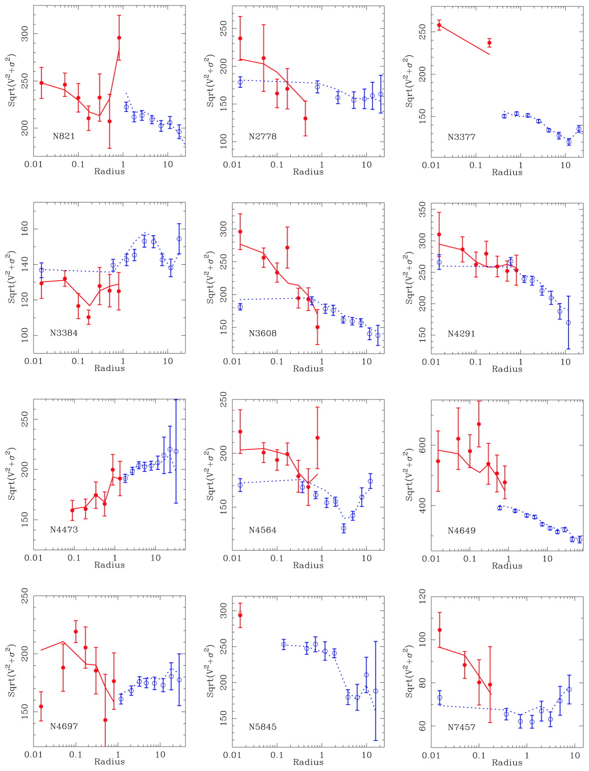
(Credit: Gebhardt et al. 2003: Velocity second moment \(\sqrt{V^2+\sigma^2}\) versus distance from the center for illustrative galaxies. The blue data points are ground-based data, while the red data have been obtained with HST. The curves are the best-fit model with SMBH, convolved with the ground-based and HST resolutions)
The HST data in red shows that the velocity dispersion remains large or increases well within the sphere of influence for these galaxies, which when included in the full orbital modeling provides strong evidence for SMBHs. The Schwarzschild models also allow us to determine the importance of the third integral and, thus, whether the two-integral models discussed above are valid. Generally, Schwarzschild models demonstrate that the ratio \(\sigma_R/\sigma_z\) varies within each galaxy, but that the average value across galaxies is \(\sigma_R/\sigma_z \approx 1\) (Gebhardt et al. 2003). As a consequence, for an individual SMBH, two-integral models can be off by a factor of a few in \(M_\bullet\), but on the whole obtain roughly the correct SMBH mass and mass distribution.
The two-integral and, later, three-integral models of dozens of SMBHs allowed their population statistics to be determined. Magorrian et al. (1998) used their large sample of SMBH masses to take a first look at the mass distribution, in particular, the distribution of the ratio \(x = M_\bullet/M_\mathrm{bulge}\). Various fits to this distribution are displayed in the following figure from their paper:
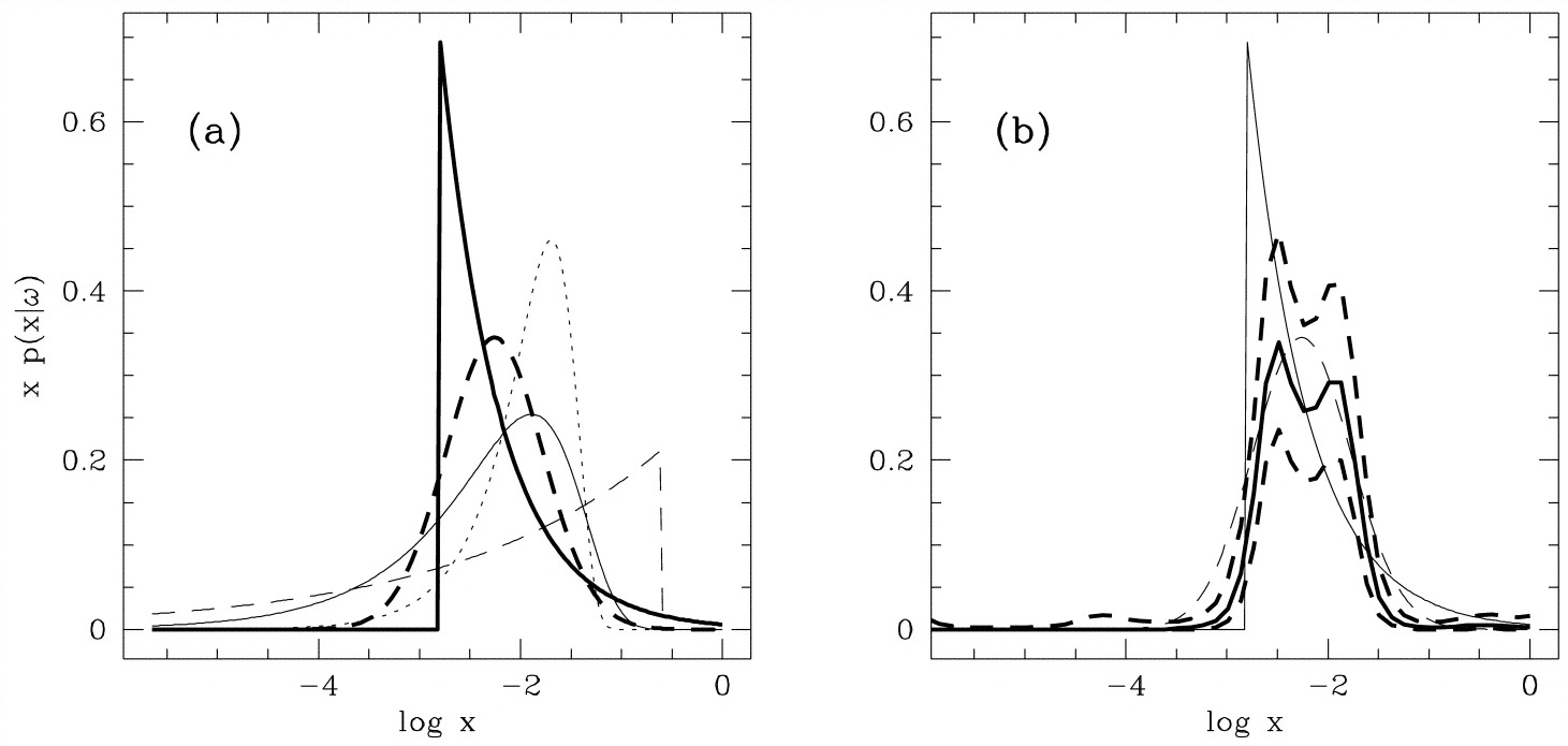
(Credit: Magorrian et al. 1998: SMBH mass distribution as a function of \(x = M_\bullet/M_\mathrm{bulge}\). The different curves in the left panel are different parametric models for the mass distribution, while the right panel shows a non-parametric reconstruction with uncertainty shown as the thick solid and dashed lines [one of the parametric models is repeated])
While the relatively small number of SMBH masses leaves some uncertainty in the exact mass distribution, both parametric and non-parametric reconstructions of the distribution of \(x\) agree that \(10^{-3} \lesssim M_\bullet/M_\mathrm{bulge} \lesssim 10^{-2}\) and SMBHs therefore are typically a few tenths of a percent of the mass of the bulge. As we saw above, this is enough to significantly change the orbital distribution within and just outside the sphere of influence, but it doesn’t directly affect the larger-scale orbital structure of the galaxy. However, the orbital distribution within the sphere of influence is correlated with the larger-scale structure of the elliptical galaxy that the SMBH lives in: The Schwarzschild models from Gebhardt et al. (2003) demonstrate that the orbits within the sphere of influence are tangentially biased for galaxies whose inner density profile is a shallow cusp (the so-called “core” galaxies discussed in Chapter 13.1) , while galaxies with a steeper inner-density cusp have kinematics that is more typically isotropic (see Chapter 14.4.2 for a discussion of the larger-scale orbital structure of these systems). Tangentially-biased orbits are consistent with the influence of a binary black hole (Faber et al. 1997) expected to form when an elliptical galaxy forms through a major merger of two smaller galaxies; as the second black hole sinks to the center, it preferentially scatters radial orbits out of the core (Nakano & Makino 1999). The more isotropic models are consistent with the black hole growing through quiescent, adiabatic growth Quinlan et al. (1995). As we will see below, this is consistent with other lines of evidence regarding the origin of the two main classes of elliptical galaxies.
The distribution of \(M_\bullet/M_\mathrm{bulge}\) above shows that, while the SMBH constitutes only a small fraction of the mass of a galaxy, its mass is closely related to the mass of the galaxy it lives in. The relation between an SMBH and its galaxy host is the area of study known as black-hole–galaxy scaling relations. In their review of the eight SMBH detections so far, Kormendy & Richstone (1995) showed that \(M_\bullet\) is correlated with the luminosity of the bulge. This started a search for the galaxy property that is most tightly correlated to SMBH mass, culminating in the discovery of the M–sigma relation: the fact that among all galaxy properties, \(M_\bullet\) appears to be most strongly correlated with the velocity dispersion of the bulge (Ferrarese & Merritt 2000; Gebhardt et al. 2000a; for an elliptical galaxy, the “bulge” is the entire galaxy). This is illustrated well in the following figure from Gebhardt et al. (2000a), which shows the correlation of \(M_\bullet\) with bulge luminosity \(L_B\) on the one hand and bulge velocity dispersion \(\sigma_e\) on the other hand; it is clear that the velocity dispersion has much smaller scatter around the power-law model than the luminosity:
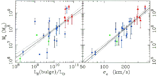
(Credit: Gebhardt et al. 2000a; the blue circles are SMBH masses derived from stellar kinematics, the green squares come from maser kinematics, and the red triangles are from gas kinematics)
The discovery of the tight relations between \(M_\bullet\) and the properties of the bulge created a rich field studying the co-evolution of SMBHs and their host galaxies (e.g., Silk & Rees 1998; Volonteri et al. 2003; Granato et al. 2004; Di Matteo et al. 2005; Croton et al. 2006; see Kormendy & Ho 2013 for a review). To better constrain the link between SMBHs and their host galaxy, much effort has been put into measuring the scaling relations between \(M_\bullet\) and \(\sigma_e\) or \(L_B\) better and into determining their intrinsic scatter (e.g., Tremaine et al. 2002). After two decades of work, it is clear that there is significant intrinsic scatter in the relation, at the level of \(0.3\,\mathrm{dex}\) in \(\log_{10} M_\bullet\), and that this intrinsic scatter is at least somewhat related to the type of galaxy (elliptical or spiral [e.g., Gültekin et al. 2009]; active or quiescient [e.g., Greene & Ho 2006]; shallow or steep inner density profile [e.g., McConnell & Ma 2013]). Because of these variations, the normalization and power-law slope of the relations depends on the sample used to measure them, but the relation found by Gültekin et al. (2009) is a reasonable typical relation
with an uncertainty in the power-law of \(0.4\), an uncertainty in the normalization of \(\approx 20\%\), and an intrinsic scatter of \(\approx0.45\,\mathrm{dex}\) in \(\log_{10}M_\bullet\) when considering all galaxy types (\(\approx 0.30\,\mathrm{dex}\) when only considering elliptical galaxies). Similarly, other relations between \(M_\bullet\) and the mass of the bulge \(M_\mathrm{bulge}\) (\(M_\bullet \propto M_\mathrm{bulge}^{1.12}\); Marconi & Hunt 2003; Häring & Rix 2004) and even with the mass of the entire dark-matter halo \(M_\mathrm{halo}\) (Ferrarese 2002) have proven to be useful.
As we discussed above using Equation \eqref{eq-ellipmass-schwarzschild-vs-sphere-influence}, measurements of the mass within the sphere of influence probe the central mass at about \(10^6\) times the SMBH’s Schwarzschild radius \(r_\bullet\) and even the high-resolution HST data do not come much closer than \(\approx 10^5\,r_\bullet\). Therefore, while the stellar kinematics measurements can establish the presence of a dense concentration of mass, they cannot unambiguously show that this concentration is in fact a black hole. So why do we believe that the central-mass concentrations in massive galaxies are black holes? All arguments for this are indirect. One argument, which was important for getting the search for SMBHs started, is that the active galactic nuclei and quasars seen at higher redshift are most easily explained as resulting from the accretion of gas onto massive black holes (e.g., Salpeter 1964; Zel'dovich 1964; Lynden-Bell 1969; Rees 1984) and evidence for the black-hole paradigm comes from such observations as the rapid variability in the quasar light and superluminal jets. Quasars were much more common at redshifts \(\gtrsim 2\) than they are in the present-day Universe and if they are powered by accretion onto a black hole, quiescent SMBHs should hide within massive galaxies today. A simple argument by Soltan (1982) (known as the Soltan argument) allows one to connect the total luminosity density of quasars at high redshift to the mass density of SMBHs today, simply by assuming that the quasar luminosity results from accretion through \(L = \varepsilon \dot{M}c^2\), where \(\varepsilon\) describes the efficiency of the accretion (which has to be \(\sim 10\%\) explain quasars, much higher than the efficiency achievable through, e.g., nuclear burning). The mass density of \(\approx 2\times 10^5\,M_\odot\,\mathrm{Mpc}^{-3}\) that one obtains from this argument (Chokshi & Turner 1992) combined with the density of massive galaxies then shows that each massive galaxy should host an SMBH with \(\approx 10^8\,M_\odot\). The consistency of this number with the observed SMBH masses and their spatial density (Merritt & Ferrarese 2001) demonstrates that SMBHs are likely the quiescient black-hole remnants of high-redshift quasars.
A further indirect argument comes from those systems where we can measure the central mass much closer to the Schwarzschild radius. Galaxies with detected nuclear masers allow the central mass to be constrained to \(r \lesssim 0.1\,\mathrm{pc}\), where the implied density is much higher. For example, the maser detection of the SMBH in NGC 4258 constrains the central mass to be \(3.6\times 10^7\,M_\odot\) within \(0.13\,\mathrm{pc}\) (Miyoshi et al. 1995); this density is so high that there is no other known stable physical system of such high density. But the best dynamical evidence for an SMBH is found in the Milky Way, where the star S2 is observed to have a Keplerian orbit with a pericenter of only \(\approx 6\times10^{-4}\,\mathrm{pc} = 120\,\mathrm{AU} \approx 1,400\,r_\bullet\) (Schödel et al. 2002; Ghez et al. 2003). Detailed measurements of S2’s orbit (and that of other, similar stars) measure the Milky Way’s SMBH to be \(M_\bullet \approx 4.3\times 10^6\,M_\odot\) (Ghez et al. 2008; Gillessen et al. 2009). The implied density is so high that it is difficult to imagine any other physical object than a black hole. Recent high-resolution interferometric observations have furthermore allowed the relativistic effects of the gravitational redshift (Gravity Collaboration et al. 2018; Do et al. 2019) and the pericenter precession (Gravity Collaboration et al. 2020) to be detected at high significance. There is thus little doubt now that the central object in the Milky Way is a black hole.
Definitive proof that the population of what we have referred to as SMBHs is in fact a population of black holes will likely have to wait until space-based interferometers like LISA are able to detect the gravitational wave signature of the inspiral and merger of binary SMBHs.
17.2. Schwarzschild modeling and the structure of elliptical galaxies
Aside from modeling the dynamics at galaxy centers and aiding in the detection and characterization of SMBHs, one of the other main uses of Schwarzschild modeling has been to study the orbital structure and the mass distribution in the inner regions of elliptical galaxies. As we discussed in Chapter 13.1, the discovery in the late 1970s that massive elliptical galaxies rotate slowly started a rich field of inquiry into the internal dynamics of elliptical galaxies. Between this and the early 2000s, the main progress in studying elliptical galaxies was on the one hand the realization that they must have significantly anisotropic velocity dispersions to satisfy the tensor-virial theorem (see Chapter 15.2), and on the other hand steadily improving observational constraints on their inner structure, isophote shapes, and kinematics. But kinematical studies remained limited to slit-based spectroscopy of one-dimensional slices along the galaxy (e.g., Binney et al. 1990), meaning that a full picture of the kinematics was lacking.
This situation changed with the development of integral-field spectroscopy (IFS), obtaining spectroscopic observations over the two-dimensional face of a galaxy in a single observation to produce a three-dimensional datacube of spectra on a two-dimensional grid (this grid may be irregular). One of the first big IFS surveys was the SAURON survey of elliptical and lenticular galaxies (Bacon et al. 2001; de Zeeuw et al. 2002). SAURON selected a representative sample of 48 objects—with galaxies chosen to cover a range of galaxy properties such as luminosity, ellipticity, and environment—to investigate the range of kinematic and stellar-population behavior in elliptical and lenticular galaxies (SAURON also observed 24 Sa galaxies, which we will not discuss here; from now on we will simple say “elliptical” galaxy, but this will typically include the lenticular SAURON galaxies as well, elliptical and lenticular galaxies are in this literature often described as early-type galaxies). The three-dimensional datacubes allow two-dimensional maps of the mean line-of-sight velocity, velocity dispersion, and higher-order moments to be extracted. A first look at the kinematic maps by Emsellem et al. (2004) immediately revealed the large diversity in kinematics among elliptical galaxies. The following figure showing the mean-velocity maps of 24 galaxies from Emsellem et al. (2007) illustrate the different types of behavior:
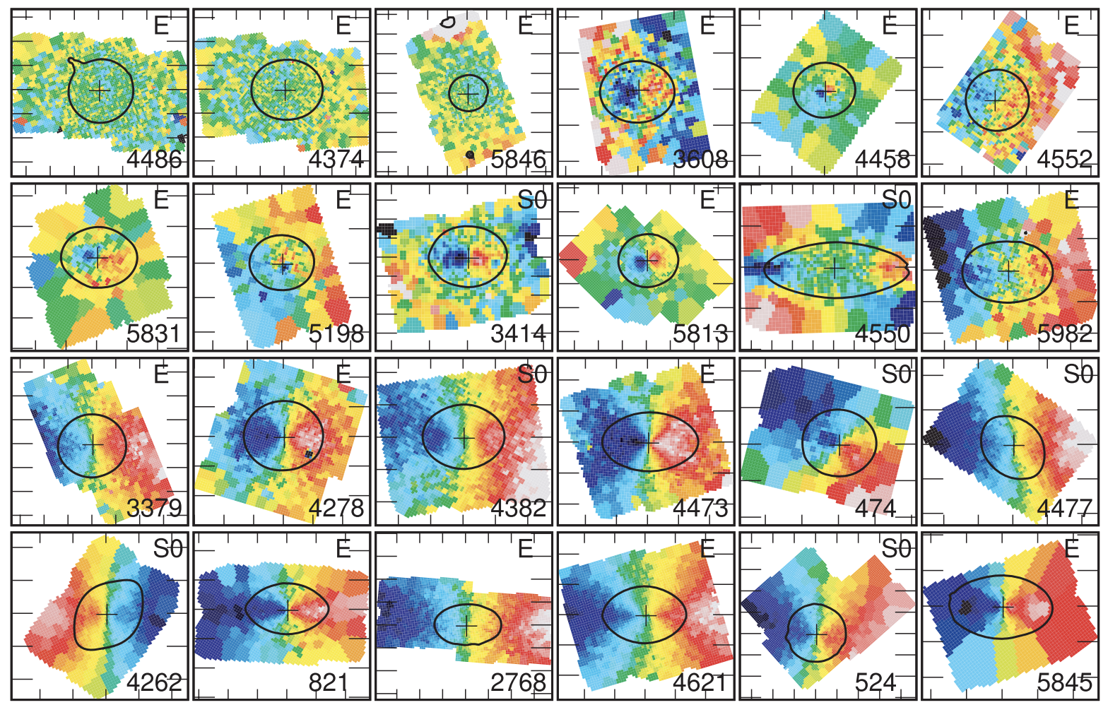
(Credit: Emsellem et al. 2007; the black contour is a representative isophote that can be used to gauge whether the kinematic major axis is aligned with the photometric major axis)
The galaxies in this figure are ordered by a measure of how much coherent rotation they show, as the progression towards more and more ordered rotation displays (ordered rotation showing up as the spider-like shape of equivelocity contours, see Chapter 9.1). The remaining 24 galaxies that are not displayed here have similar ordered rotation as the last few in this figure. Thus, it is clear that many elliptical galaxies display ordered rotation aligned with the photometric axes and only a small fraction (about 25% based on the figure above) have velocity fields where the velocity is either entirely disordered or where there are signs of rotation, but they are not coherent throughout the galaxy. Only the first three galaxies display no signs of rotation, while the remaining galaxies in the first two rows either have so-called kinematically-decoupled cores (KDCs; Bender 1988; Jedrzejewski & Schechter 1988), with rotation limited to the very center of the galaxy, counter-rotating disks with rotation opposite to the overall rotation sense of the galaxy (e.g., Rubin et al. 1992; Rix et al. 1992), or a sort of “disordered ordered motion”.
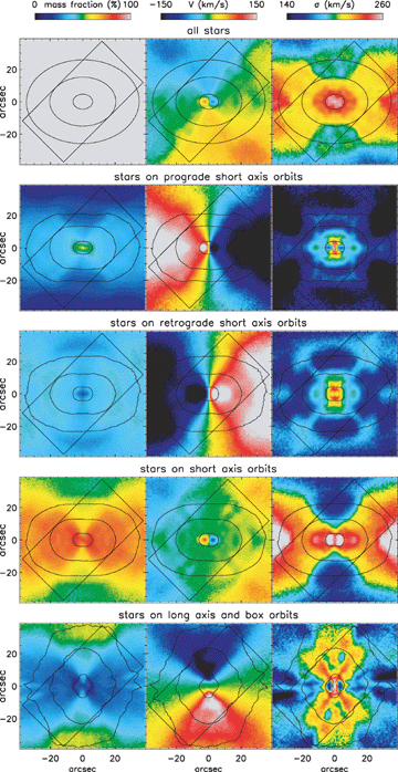
The wealth of data means that we can use Schwarzschild modeling usefully to recover the orbital distribution in great detail. In light of our discussion of the different orbit families in triaxial galaxies in Chapter 14.4, of particular interest is the study of van den Bosch et al. (2008). They implemented a triaxial version of Schwarzschild’s technique (a difficult task as discussed in Chapter 15.3.3) and used it to determine the internal orbital distribution of NGC 4365, an E3 galaxy with a kinematically-decoupled core and a strong misalignment between the kinematic and photometric major axes. The data compared to the best-fit model are shown in the following figure:
(Credit: van den Bosch et al. 2008; the top row has the data, the middle row the data point-symmetrized relative to the center, and the bottom row has the Schwarzschild model)
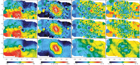
The data and the model here are represented as the first four moments of the line-of-sight velocity distribution: the mean velocity, velocity dispersion, and the \(h_3\) and \(h_4\) Gauss-Hermite moments (van der Marel & Franx 1993). The kinematics clearly show that NGC 4365 has to be triaxial, because of the minor-axis rotation: the large-scale rotation pattern is aligned with the minor photometric axis (isophotes are shown as contours), rather than with the major axis; only the KDC rotation is aligned with the major photometric axis. The Schwarzschild model provides an excellent fit to the data. We can then use the best-fit Schwarzschild model to look at how the different orbital families contribute to the total density and velocity maps. This is shown in the next figure:
(Credit: van den Bosch et al. 2008)
The top row displays the combined density, mean velocity, and velocity dispersion from all orbits, while the other rows show the contributions from different orbit families, focusing on the properties of the short-axis tube orbits. The short-axis tube orbits dominate the mass density almost everywhere, but they are made up of a prograde and a retrograde component that are almost equivalent aside from their sense of rotation and, therefore, almost cancel each other’s rotation signal out. Only at the center does this cancellation not happen and the result is the KDC. While the short-axis tubes also give rise to a retrograde overall rotation on larger scales, this is drowned out by the much larger contribution of the long-axis tubes and the resulting rotation pattern on large scales is strongly misaligned with the photometric axes. The orbital structure of NGC 4365 therefore demonstrates how combining the basic orbit families in triaxial potentials can lead to a complex pattern of rotation and velocity dispersion in galaxies.
A closer inspection of the mean-velocity fields from Emsellem et al. (2007) above shows that most elliptical galaxies in the SAURON sample do not call for a triaxial analysis, because their kinematics is in most cases aligned with their photometry. For this reason, the SAURON galaxies have not been studied with triaxial modeling, but instead with simple two-integral (Jeans) or three-integral (Schwarzschild) axisymmetric modeling similar to the SMBH analyses discussed in the previous section. Krajnović et al. (2005) performed a detailed axisymmetric, three-integral Schwarzschild analysis of NGC 2974 and demonstrated that the modeling was able to recover the intrinsic orbital distribution for mock data with similar properties as the best-fit Schwarzschild model to the data. The tests also show that the mass-to-light ratio can be reliably determined using Schwarzschild modeling, but that the inclination is only weakly constrained; the inferred mass-to-light ratio from kinematic data is therefore only weakly dependent on the inclination, a useful property, because it removes the inclination bias that in other situation severely affects inferred properties (such as the intrinsic shape of a galaxy!).
That most SAURON elliptical galaxies can be satisfactorily modeled using three-integral Schwarzschild modeling poses another question: whether they can be modeled using the even simpler two-integral modeling. As we discussed in the previous section, the advantage of two-integral modeling is that the even part of the distribution function \(f(E,L_z)\) is uniquely determined by the density and the odd part by the mean velocity. This means that two-integral models are far easier to implement and fit to data, because we can compute all observable moments of the distribution function using the axisymmetric Jeans equations starting from the (deprojected) density and average rotation velocity \(\overline{v_\phi}(R,z)\), rather than performing computationally-expensive Schwarzschild modeling. The basic answer is that two-integral modeling both does and does not suffice to describe the observed kinematics of elliptical galaxies. It can reliably recover quantities such as the total mass-to-light ratio (Cappellari et al. 2006). But as we saw in Chapter 15.2, elliptical galaxies must deviate from the \(\sigma_z = \sigma_R\) relation inherent in two-integral modeling for their observed shapes to be consistent with their low bulk velocities (this is the case even for most of the elliptical galaxies that display strong rotation). Cappellari et al. (2007) demonstrated this explicitly using three-integral Schwarzschild modeling of a subset of 24 elliptical galaxies in SAURON.
That the mass-to-light ratio can be consistently determined using two- and three-integral Schwarzschild modeling allows one to look for trends in mass-to-light ratio with other galaxy properties. The \(I\)-band mass-to-light ratios \(M/L\) determined by Cappellari et al. (2006) span a range of \(1 \lesssim M/L < 6\) and they are strongly correlated with the luminosity-weighted second moment \(\sigma_e\) of the line-of-sight velocity distribution within the effective radius as
with a scatter of only \(\approx 0.2\,\mathrm{dex}\) in \(\log_{10} M/L\) at a given \(\sigma_e\). This is a similar relation as the M-sigma relation for SMBHs and their host velocity dispersion. The variation in the mass-to-light ratio inferred from the dynamical analysis is partly due to changes in the dark-matter contribution within the effective radius, which is higher for more massive galaxies. But the main reason for the difference in \(M/L\) is a changing stellar population with galaxy mass, with more massive galaxies having older populations with higher \(M/L\) than less massive galaxies. The tight relation between \(M/L\) and \(\sigma_e\) furthermore has implications for the most important scaling relation for elliptical galaxies, the fundamental plane: a tight relation between the effective radius, velocity dispersion, and the surface brightness at the effective radius (Djorgovski & Davis 1987; Dressler et al. 1987). Under the assumption of constant \(M/L\) and orbital structure, the fundamental plane can be derived using the virial theorem, but there is an offset between the virial-theorem prediction and the actually observed relation, known as the tilt of the fundamental plane. The \(M/L-\sigma_e\) relation can explain 90% of this tilt, demonstrating that the tilt is mainly due to differences in \(M/L\) rather than significant differences in the orbital structure among elliptical galaxies. We will discuss the fundamental plane in more detail in Part IV.
The SAURON survey thus demonstrated that elliptical galaxies display an interesting variety in observed kinematics, including completely disordered motion, various degrees of more ordered kinematics, and clean rotational systems. SAURON further showed that quantities derived from the two-dimensional kinematic maps such as the orbital anisotropy and the mass-to-light ratio contain important information about the formation and evolution of elliptical galaxies. As is often the case, the way forward was to go from the representative SAURON sample to statistical samples that are selected in a well-defined manner from the parent galaxy population and that therefore can be related back to the full population. However, the SAURON analyses also showed that two-integral modeling does not suffice to fully describe the observed kinematics, but Schwarzschild modeling is computationally-expensive and labor-intensive and therefore difficult to apply to the much larger statistical samples. However, it turns out that there is a simple way to generalize the two-integral method to an effective three-integral method that retains the simplicity of the two-integral modeling, but also attains the realism of the three-integral Schwarzschild modeling. We discuss this in the next section.
17.3. Jeans Anisotropic Modeling (JAM)
There are only a small number of analytic three-integral \(f(E,L_z,I_3)\) distribution functions for axisymmetric, elliptical-galaxy-like systems and these are not particulary realistic representations of actual elliptical galaxies. To perform three-integral steady-state dynamical modeling of elliptical galaxies, we therefore either need to use the Schwarzschild orbit-superposition technique or use the Jeans equations. Because Schwarzschild modeling is computationally-expensive and complex to implement and apply, Jeans modeling is preferred for uniform analyses of large samples of galaxy kinematics. However, while two-integral Jeans modeling has a unique solution for a given density, gravitational potential, and mean-rotation field as we discussed in the previous sections, three-integral Jeans modeling does not have a unique solution. This is a manifestation of the fact that the Jeans equations in general do not close as discussed in Chapter 6.4 : in general there is an infinite number of distribution functions in a given gravitational potential that give rise to the same density and mean rotation pattern and this remains the case even if we assume that the system is axisymmetric.
To use the Jeans equations, we therefore have to make a closure assumption to make the Jeans equations return a unique answer. Two-integral Jeans modeling provides an example of this: by assuming that the distribution function has the form \(f(E,L_z)\), we have that \(\overline{v_R^2} = \overline{v_z^2}\) and \(\overline{v_R\,v_z} =0\), and the two axisymmetric Jeans equations (11.8) and (11.9) then only have two unknowns: \(\sigma_z^2 = \sigma_R^2 = \overline{v_R^2} = \overline{v_z^2}\) on the one hand and \(\overline{v_\phi^2}\) on the other. We can therefore solve for all of the second moments. An additional assumption is necessary to separate \(\overline{v_\phi^2}\) into the contribution from ordered rotation, \(\overline{v_\phi}^2\), and that from the velocity dispersion, \(\sigma_\phi^2\), through \(\overline{v_\phi^2} = \overline{v_\phi}^2 + \sigma_\phi^2\). With this additional assumption, we can determine all first moments (keeping in mind that \(\overline{v_R} = \overline{v_z} = 0\)).
We can close the Jeans equations for three-integral models \(f(E,L_z,I_3)\) by making similar assumptions about the different components of the mean velocity and the velocity dispersion tensor. The idea behind Jeans anisotropic modeling (JAM; Cappellari 2008) is to assume that the system has a constant anisotropy \(\beta_z\) in the meridional plane, defined similarly to the radial anisotropy for spherical systems from Equation (6.51)
such that \(\overline{v_R^2} = (1-\beta_z)^{-1}\overline{v_z^2}\) (the second equality holds because \(\overline{v_R} = \overline{v_z} = 0\) for an axisymmetric system). Additionally, we assume that \(\overline{v_R\,v_z} =0\) similar to the two-integral case. The latter assumption is equivalent to assuming that the velocity-dispersion tensor is diagonal in the cylindrial coordinate frame. The two-integral \(f(E,L_z)\) models are then simply obtained by setting \(\beta_z=0\), while for \(\beta_z\neq0\), the dispersion tensor is anisotropic. With these assumptions and the boundary condition that \(\nu\,\overline{v_z^2} \rightarrow 0\) as \(|z| \rightarrow \infty\), the axisymmetric Jeans equations (11.8) and (11.9) have the following solution
As before, to also determine the first moment \(\overline{v_\phi}\), we need an additional assumption about how \(\overline{v_\phi^2}\) separates into \(\overline{v_\phi}^2\) and \(\sigma_\phi^2\). There are different options for how to do this, but one obvious one is to use a parameter that characterizes the deviation from isotropy in the radial and tangential directions, by defining
such that then
This closure of the axisymmetric Jeans equations forms the backbone of the JAM method. A practical application of this method further needs to deal with the deprojection of the observed surface-brightness profile, the calculation of the gravitational potential from the deprojected profile, and the calculation of the integrals in the previous sets of equations. A solution to all of these issues is to use the multi-Gaussian expansion (MGE) of the surface brightness described in Chapter 15.3.3. As we discussed there, a sum of Gaussians can represent almost any observed galaxy profile and is straightforward to deproject for any assumed inclination. The gravitational potential of the deprojected profile can be computed using the methods of Chapter 13.2. Furthermore, Cappellari (2008) demonstrated that the integrals in the expressions for the first and second moments above can be significantly simplified to a single numerical quadrature for each quantity and they are therefore quick to compute, and that the projection of the three-dimensional kinematics onto the line of sight can be computed in a similar way. By representing a central black hole or a dark matter halo as a single or sum of Gaussians as well, the MGE formalism can be used to build realistic models of galaxies from their innermost regions to their outskirts. Thus, the MGE formalism provides a quick way to realistically model the kinematics of observed external galaxies. As with all use of the Jeans equations, there is no guarantee that there exists a distribution function \(f(E,L_z,I_3)\) with the kinematics given by the solution of the Jeans equation, but the results from Schwarzschild modeling of SAURON galaxies demonstrate that consistent \(f(E,L_z,I_3)\) models with similar kinematics as the JAM models exist (e.g., Cappellari et al. 2007).
17.4. The inner orbital structure of elliptical galaxies
To better understand the internal structure of elliptical galaxies and their stellar populations, SAURON was followed by the larger, statistical ATLAS\(^{\mathrm{3D}}\) survey (Cappellari et al. 2011). The ATLAS\(^{\mathrm{3D}}\) survey is statistical in the sense that it selects a sample of galaxies for detailed integral-field spectroscopy based on a simple combination of selection criteria applied to a complete parent sample of galaxies. Briefly, the ATLAS\(^{\mathrm{3D}}\) survey consists of all early-type galaxies (elliptical and lenticular) within 42 Mpc that are observable from the William Herschel Telescope on La Palma, are away from the Milky Way’s mid-plane, and that have an absolute 2MASS \(K_s\) band magnitude \(M_K < -21.5\) (corresponding to a stellar mass \(M_* \gtrsim 6\times 10^9\,M_\odot\)). These selection criteria give 871 galaxies, with 192 lenticular galaxies (22 percent) and 68 elliptical galaxies (8 percent; we will again simply refer to all of these as “elliptical galaxies”); only the elliptical and lenticular galaxies were followed up with IFS observations.
As with the SAURON sample, it is instructive to first simply consider the kinematic maps to get a sense of the range of kinematic behavior among elliptical galaxies. Because the ATLAS\(^{\mathrm{3D}}\) sample is statistical, we can now quantitatively determine the occurrence of different types of kinematics. Krajnović et al. (2011) did this by applying a method, kinemetry, to the mean line-of-sight velocity maps. Kinemetry is similar to the method discussed in Chapter 13.1 to determine whether an elliptical galaxy is boxy or disky, in that one fits elliptical profiles to the kinematic map and then determines whether higher-order harmonics are present in the kinematics or not. This is motivated by the fact that many elliptical galaxies display rotation signatures (see Section 17.2), for which the expected line-of-sight velocity is \(V(x,y) = V_0 + v_\phi(R)\,\cos\theta\,\sin i\); we derived this relation for a thin disk in circular rotation in Chapter 9.1.2 (see Equation 9.2), but allow here for a rotation velocity \(v_\phi\) that is different from the circular velocity, because the rotation speed in elliptical galaxies is much less than the circular velocity. By fitting the parameters of this basic form (the ellipse’s center, \(\cos i\), and the position angle of the major axis at the receding-velocity side, known as the kinematic position angle), we can determine how regular the rotation pattern of a given galaxy is. Deviations from simple rotation can come in different forms: smooth or abrupt changes in the kinematic position angle, multiple maxima in \(v_\phi(R)\), or an absence of clear rotation (parameterized through the relative strength \(k_5/k_1\) of the amplitude of the \(\sin (5\theta)\) and \(\cos (5 \theta)\) terms, \(k_5\), with respect to \(k_1 = v_\phi(R)\,\sin i\)). Krajnović et al. (2011) classify galaxies with average \(k_5/k_1 < 0.04\) as regular rotators (RR), while other galaxies are non-regular rotators (NRR). Abrupt changes in the kinematic position angle are associated with a kinematically-decoupled core (KDC) or even a counter-rotating core (CDC; when the position angle changes by \(180^\circ\)), while smooth changes in position angle are kinematic twists (KT). Galaxies with no deviations are classified as “no feature” (NF), while those with simply very small rotational velocities have “low velocity” (\(k_1 < 5\,\mathrm{km\,s}^{-1}\)), and those with two maxima as “2M”. Finally, some galaxies have multiple peaks in their velocity dispersion and are denoted by “\(2\sigma\)”. Examples of the way that these different kinematic features manifest themselves in ATLAS\(^{\mathrm{3D}}\) galaxies are given in the following figure, where the black lines are contours of the photometric observations:
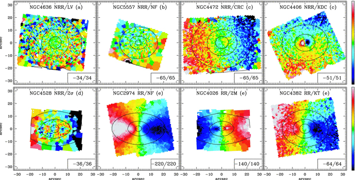
(Credit: Krajnović et al. 2011)
From looking at all 260 ATLAS\(^{\mathrm{3D}}\) galaxies and considering the way in which the various kinematic features appear and correlate with each other, Krajnović et al. (2011) divided the sample in five kinematic groups. Approximately 80% of the galaxies has regular rotation or is close to it (meaning that the galaxy is a regular rotator with either no feature, two \(v_\phi\) maxima, or a smooth kinematic twist). Another \(\approx 7\%\) have a kinematically-decoupled core or a counter-rotating core, and a further \(\approx4\%\) are characterized by multiple dispersion peaks. Finally, \(\approx 7\%\) of galaxies are non-regular rotators with either low velocity or no feature. The various statistics on the kinematics of elliptical galaxies are shown in the following pie charts:
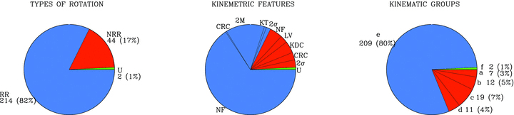
(Credit: Krajnović et al. 2011; left: regular rotator (RR) vs. non-regular rotator (NRR); middle: prevalence of different kinemetric features (see above); right; fraction of different kinematic groups: (a) NRR/LV, (b) NRR/NF; (c) KDC or CRC, (d) \(2\sigma\), (e) RR/NF, RR/2M, RR/KT, (f) unclassified [U])
Thus, one of the main take-aways from this detailed look at the kinematics of elliptical galaxies is that \(\approx 80\%\) of them have quite regular rotation. The remaining \(20\%\) have complex kinematics that is indicative of a complex orbital structure that is likely triaxial. Dynamical modeling of the latter group requires Schwarzschild modeling to deal with the complexity of the observed kinematics, but for the former group that makes up the vast majority of the sample, the simpler JAM modeling from the previous section suffices (as shown by comparing JAM and Schwarzschild models for galaxies of this type; Cappellari 2008).
The detailed IFS observations of elliptical galaxies by SAURON and ATLAS\(^{\mathrm{3D}}\) also lets us reconsider the question of how much of the shape of the elliptical galaxies is due to rotational flattening versus anisotropic random motions. We first discussed this in Chapter 15.2, where we concluded that the flattened, oblate shapes of elliptical galaxies cannot solely be due to rotational flattening of an isotropic rotator, because the observed rotation velocities are too small to support the oblate shape. The next simplest model is that of an anisotropic rotator, where the velocity dispersion is smaller in the direction along which the density is flattened, which we’ll take to be the \(z\) axis. In terms of the contribution to the kinetic energy tensor from random motions, \(\vec{\Pi}_{\alpha\beta}\) (see Equation 15.18), this means that \(\Pi_{zz} < \Pi_{RR}\) or that the following anisotropy parameter
is larger than zero. Note that this definition is similar to that of \(\beta_z\) in JAM models, Equation \eqref{eq-ellipmass-anisotropybetaz-jam}; indeed, under the JAM assumption of constant \(\sigma_z\) and \(\sigma_R\), the two are equal. But the advantage of the definition from Equation \eqref{eq-ellipmass-anisotropybetaz-kintensor} is that it can be computed for Schwarzschild models as well.
With full dynamical models, we can turn the \(v/\sigma\) versus ellipticity diagram that we discussed in Chapter 15.2 into a similar anisotropy \(\beta_z\) versus intrinsic ellipticity diagram that contains direct information on the orbital structure of galaxies. This is shown for a set of Schwarzschild and JAM models in the following figure:
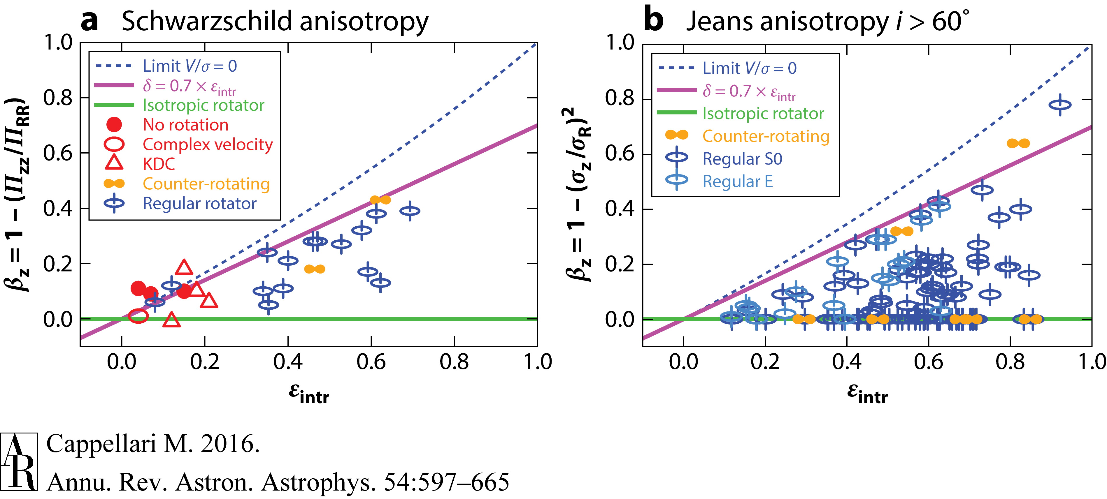
(Credit: Cappellari 2016)
The first thing to notice is the similarity between the diagram obtained with Schwarzschild modeling and that with the simpler JAM models. This is another indication that JAM models suffice to capture the main behavior of the dynamics of a wide range of elliptical galaxies. The dashed line shows the locus of galaxies that are entirely supported by an anisotropic velocity dispersion and have no rotation. All galaxies that are significantly flattened, \(\varepsilon \gtrsim 0.3\), lie well below this line and there seems to be an upper limit to their anisotropy given by the purple line. We also see that the regular rotators are the only elliptical galaxies that are significantly flattened intrinsically and that they are by and large quite anisotropic, although the JAM models show that a subset of them can be explained as pure isotropic rotators. Galaxies without a clear rotation pattern are generally close to round and they require therefore little anisotropy to support their shapes. However, the left panel also demonstrates that these are the galaxies with complex kinematics and kinematically-decoupled cores, indicating that they are most likely triaxial.
Finally, we can introduce one more useful quantity to characterize the dynamical structure of elliptical galaxies, a proxy for the projected specific angular momentum of stars in the galaxy defined as (Emsellem et al. 2007)
where \(V\) and \(\sigma\) are the mean and velocity dispersion of the line-of-sight velocity distribution and the averages are over a two-dimensional region of the galaxy. The region is typically that within the effective radius, in which case the parameter is also denoted as \(\lambda_{R_e}\). As a proxy for the specific angular momentum, \(\lambda_R\) is good at distinguishing galaxies with significant rotation and \(\lambda_{R_e}\) is therefore used to quantitatively distinguish slow rotators with \(\lambda_{R_e} \lesssim 0.1\) from fast rotators with \(\lambda_{R_e} \gtrsim 0.1\). Additionally, slow rotators only exist at \(\varepsilon_\mathrm{obs} < 0.4\). The following figures displays the distribution of elliptical galaxies in the \((\varepsilon_\mathrm{obs},\lambda_{R_e})\) plane with symbol colors and shapes showing other crucial properties of the galaxies:
|
|
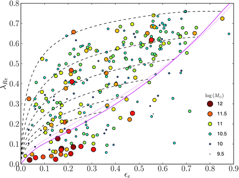

(Credit: left: Emsellem et al. 2011; right; Cappellari 2016)
Comparing these figures to the anisotropy figures above, it is clear that \(\lambda_{R_e}\) is able to separate the dynamically-distinct regular rotators and non-regular rotators very well, without requiring any dynamical modeling.
The results discussed in this and the previous sections therefore clearly show that there are two distinct classes of elliptical galaxies in the present-day Universe. On the one hand there are the fast rotators that display regular rotation fields that can be well modeled as anisotropic, axisymmetric rotators that are in many ways simply puffed-up disks. The figure above demonstrates that fast rotators dominate the elliptical-galaxy population at the lower stellar-mass end of \(M_* \lesssim 2 \times 10^{11}\,M_\odot\). The right-hand panel furthermore demonstrates that the fast rotators almost entirely encompass the population of power-law galaxies, those galaxies with power-law inner density profiles. While the correspondence is not as good as for other quantities, fast rotators also preferentially have disky isophotes rather than boxy isophotes (Emsellem et al. 2007).
On the other hand we have the slow rotators, which have complex velocity fields characterized by either an absence of coherent rotation or by multiple kinematic components such as kinematically-decoupled cores. The figures above demonstrate that slow rotators dominate the population at high stellar mass, \(M_* \gtrsim 2 \times 10^{11}\,M_\odot\), and that they typically display central-density cores. Thus, this all points towards slow rotators being triaxial, because triaxiality is required to explain their complex kinematics and their inner core structure allows for triaxiality to be straightforwardly supported (see Chapter 14.4). However, their observed ellipticity is \(\varepsilon_\mathrm{obs} < 0.4\) and their intrinsic ellipticity is therefore typically small. Taken together with the fact that their orbital anisotropy is similary small, this indicates that while they are triaxial, they do not strongly deviate from spherical symmetry.
Slow rotators are commonly found in dense environments, such as the centers of groups and clusters, while fast rotators are more generally found in the field like spiral galaxies. Because the slow and fast rotators are distinct in their properties, they likely indicate two different formation mechanisms for elliptical galaxies. The triaxial, cored structure of slow rotators in dense environments is most easily explained as the product of gas-poor major mergers between two galaxies, where the collisionless merger leads to a triaxial final configuration (in much the same way as dark-matter halos in collisionless simulations are triaxial). As we saw in Section 17.1 above, the orbital structure near the central SMBH provides further evidence for this picture, because the central radial orbits appear to have been scoured by the inspiral of a second SMBH. Fast rotators likely build up much of their mass through gas accretion, much like spiral galaxies, but unlike spirals their star formation is shut off for a variety of reasons (such as the inability to accrete gas after falling into a cluster or group, or feedback from their central SMBH). Growing further through minor mergers, their disks are destroyed and they are puffed up into the observed oblate rotators, but they retain signatures of their origin in the form of disky isophotes and an isotropic orbit distribution around their SMBH. Observations of the age and abundance distribution of elliptical galaxies of different masses and in different environments corroborate this picture (e.g., Thomas et al. 2005; Conroy et al. 2014), with the higher-mass, slow rotators consisting of uniformly old stars enhanced in alpha elements such as oxygen and magnesium, indicative of an early assembly before the gas-poor merger(s) that lead to the final triaxial massive elliptical; while lower-mass, fast rotators have stars with a wider range of ages and the solar-like oxygen/magnesium abundances that result from the more stable star-formation history driven by gas accretion.
17.5. The stellar and dark mass profiles of elliptical galaxies
Unlike disk galaxies, elliptical galaxies do not typically have thin, rotating gas disks that allow the rotation curve and enclosed mass profile to be determined with relative ease (see Chapter 9). Even in the fast rotators, the velocity dispersion provides a significant part of the support of an elliptical galaxy, such that the rotational velocity differs significantly from the circular velocity. We therefore have to resort to other methods to determine the overall mass distribution within elliptical galaxies and to separate it into the contribution from luminous and dark-matter components. In this section, we discuss how a consistent picture of the mass distribution in elliptical galaxies emerges from the combination of dynamical modeling of stellar kinematics with gravitational lensing of the strong, weak, and micro varity. We already described the basic methods and results from dynamical modeling of stellar kinematics in the previous sections, so we’ll focus on results from gravitational lensing here and discuss their relation to results from dynamical modeling along the way.
In Chapter 16.2.4, we discussed how strong lensing allows the mass within the Einstein radius to be determined in a manner that does not require assumptions of equilibrium like dynamical modeling. Einstein radii for low-redshift lenses are a few kpc (see Equation 16.63), similar to the effective radius of the light profile. Strong lensing therefore constrains the mass in the region where stars contribute significantly to the gravitational potential. However, we also saw in Chapter 16.2.4 that strong lensing is affected by the mass-sheet degeneracy, meaning that the fraction of the mass within the Einstein radius that is associated with the lens galaxy cannot be unambiguously determined. And we saw that strong lensing cannot measure the enclosed mass over a wide range of radii, but is instead limited to the mass distribution around the Einstein radius. Thus, strong lensing needs to be combined with other methods like stellar kinematics to break the mass-sheet degeneracy and to extend the mass profile measurement to smaller and larger radii.
Many strongly-lensed systems exists and their mass distributions have been analyzed, but a particularly interesting and comprehensive set of observations and analyses was performed by the Sloan Lens ACS Survey (SLACS; Bolton et al. (2006)). SLACS selected a large sample of galaxy-galaxy lenses by looking for galaxy spectra in the spectroscopic database of the Sloan Digital Sky Survey (SDSS; York et al. 2000; Eisenstein et al. 2001; Strauss et al. 2002) that have multiple nebular emission lines at a redshift significantly higher than that of the SDSS target galaxy, indicating that the spectrum contains a background galaxy that is likely lensed. These candidates were then followed up with the Hubble Space Telescope’s Advanced Camera for Surveys (ACS) instrument to obtain the high-resolution imaging that can reveal whether a lensed background galaxy is in fact present. Through this procedure, SLACS discovered 70 strong-lensing systems (Bolton et al. 2008a), with many of them displaying an Einstein ring, indicating that the background source galaxy is almost exactly behind the lens galaxy. A few examples are shown in the following figure:
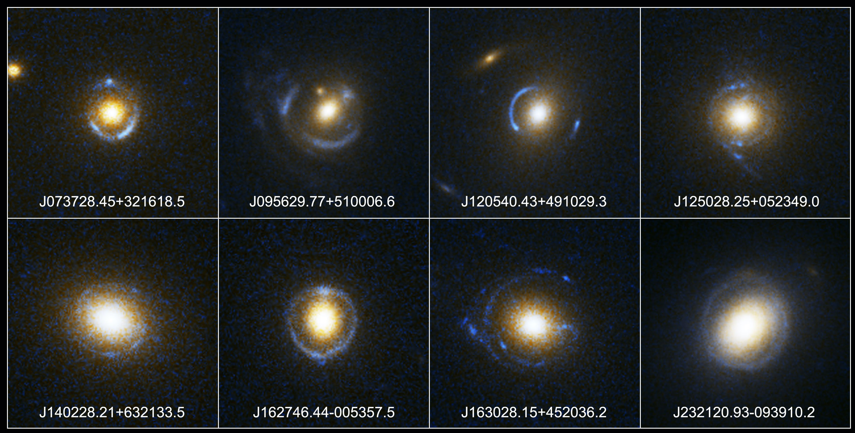
(Credit: NASA, ESA, and the SLACS Survey team)
The way that the SLACS lenses are found has two important implications for their use to constrain the mass distribution in elliptical galaxies. Firstly, because the lensed source galaxy is found as a second set of lines in a galaxy spectrum, the redshift of both the source and the lens is known from the outset. This is often not the case for other strong lensing systems, where either the lens or the source is too faint to obtain a spectroscopic redshift or where it simply requires expensive follow-up observations. Secondly, the SDSS spectrum of the lens also allows the velocity dispersion of the lens to be measured, which can be combined with the radius of the Einstein ring to break the mass-sheet degeneracy and constrain the mass profile through dynamical modeling. SDSS fibers have a diameter of \(3''\), so the velocity dispersion is measured within a similar radius as the Einstein ring (which has a diameter of \(\approx 2''\)).
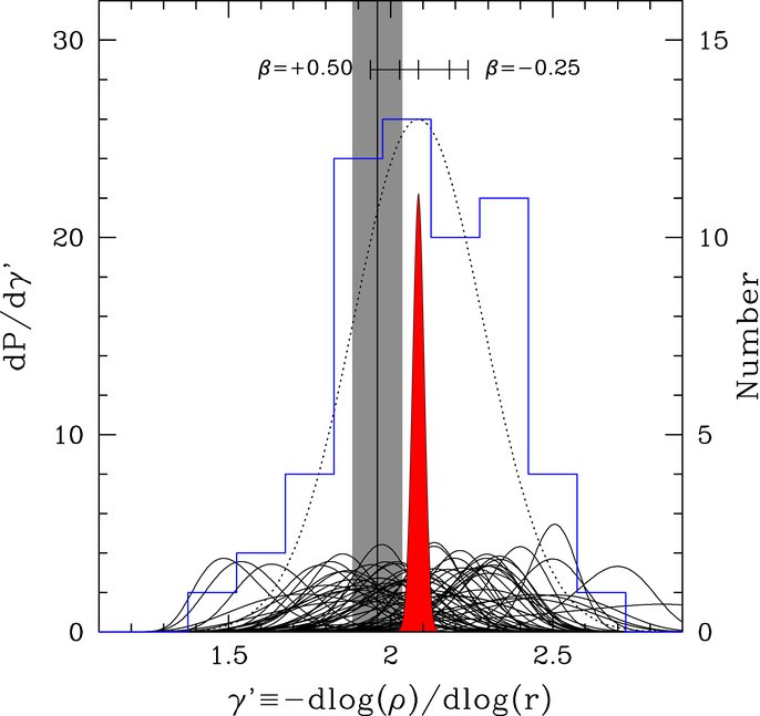
Koopmans et al. (2009) analyzed 58 SLACS lenses combining the lensing and velocity dispersion measurements to determine the logarithmic slope of the total mass profile, approximated as a single power law \(\rho(r) \propto r^{-\gamma'}\). First using the observed Einstein rings to determine the mass within the Einstein radius, they then obtain the velocity dispersion by solving the spherical Jeans equation (6.53) for different constant values of the anisotropy \(\beta\), modeling the luminous component as a massless Hernquist or Jaffe profile with half-light radius determined by the observed profile (e.g., Treu & Koopmans 2002); the observed velocity dispersion within the \(3''\) SDSS fibers is obtained by projecting the velocity dispersion onto the line of sight and averaging it using the surface-brightness profile (see Equation 7.17). Combining the lensing and dynamical-modeling constraints, the resulting determinations of the logarithmic slope of the mass profile are shown in the left-hand panel of the following figure:
|
|
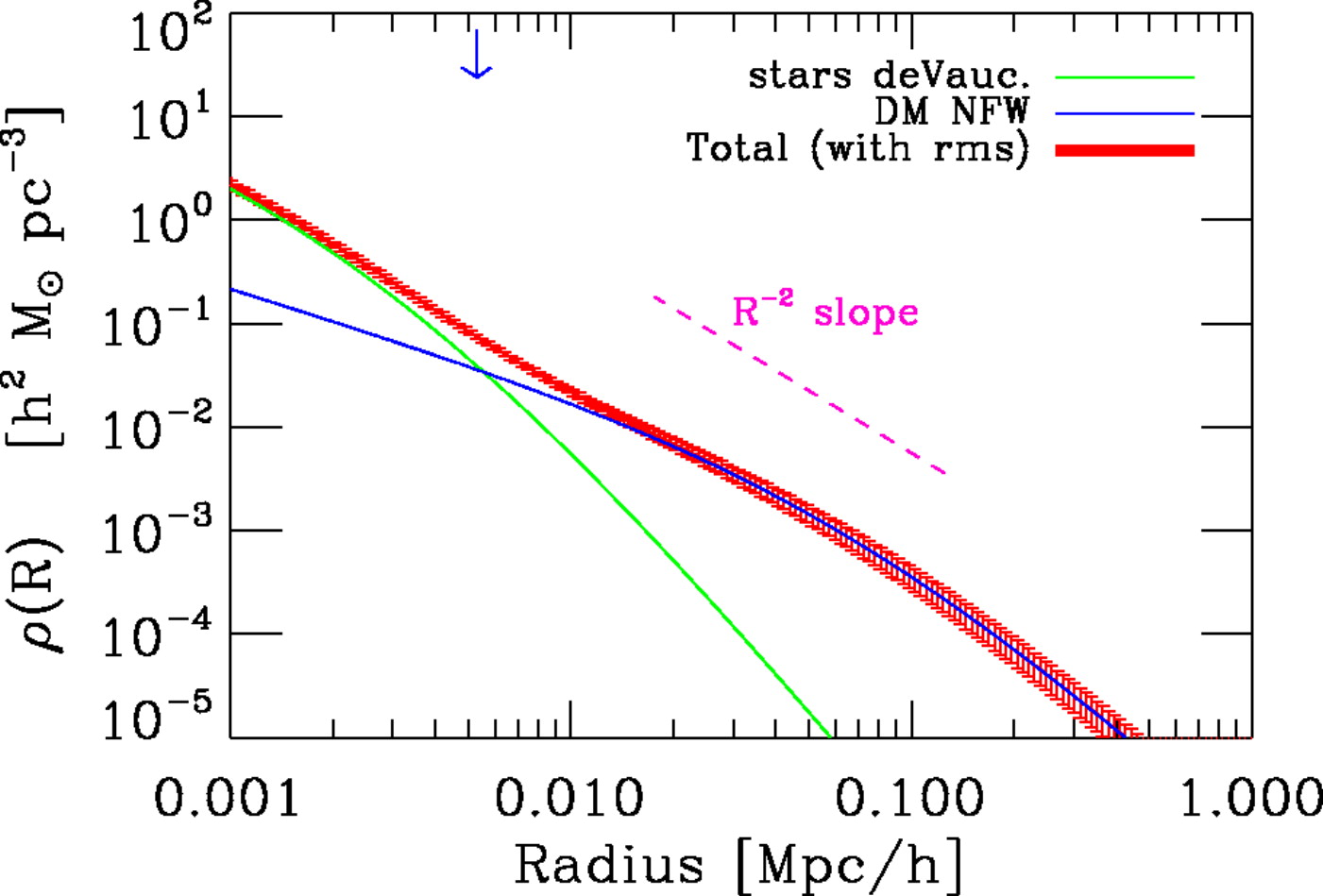
(Credit: left: Koopmans et al. 2009; right; Gavazzi et al. 2007)
While the uncertainties in the individual \(\gamma'\) measurements are large, they all scatter around \(\gamma' \approx 2\). A joint analysis of all systems assuming \(\beta = 0\) and that they have a \(\gamma'\) drawn from a Gaussian with scatter \(\sigma_{\gamma'}\) shown by the red histogram gives \(\gamma' = 2.085\pm 0.025\) and \(\sigma_{\gamma'} = 0.20\pm0.03\). Dynamical-modeling-only analyses of the kinematics of stars (e.g., Cappellari et al. 2015), which can also be combined with planetary nebulae that can be seen to larger distances (e.g., de Lorenzi et al. 2008), find the same result. Thus, the total mass profile of elliptical galaxies near the Einstein radius is approximately \(\rho(r) \propto r^{-2}\). This spherical density corresponds to a flat rotation curve (see Chapter 3.4.5) or, equivalently, a singular isothermal sphere. Thus, the rotation curves of elliptical galaxies in the region where stars contribute significantly to the potential is flat just like for spiral galaxies (Chapter 9). This is remarkable given that otherwise their spatial and dynamical structure is so different!
To extend the measurement of the total mass profile to significantly larger radii, we need to use weak lensing. As we discussed in Chapter 16.3.4, the weak lensing signal from individual, even massive, galaxies is so weak that it is difficult to detect. But selecting a population of lens galaxies and assuming that they all share the same mass profile, shape measurements of background sources behind all lens galaxies can be combined to determine the typical mass profile of the population of lens galaxies. We can do this therefore for the SLACS sample of massive elliptical galaxies. As is the case with strong lensing, weak lensing suffers from the mass-sheet degeneracy, but since a mass-sheet adds a constant surface density, we can robustly determine changes in the surface density between different parts of galaxies and thus measure the profile. Gavazzi et al. (2007) presented such an analysis for 22 SLACS lenses and determined the mass profile out to \(\approx 400\,\mathrm{kpc}\), shown in the right panel of the figure above. It is clear from the figure that they find that the \(\rho(r) \propto r^{-2}\) behavior extends all the way to the edge of their data, demonstrating that massive elliptical galaxies are approximately singular isothermal spheres from their Einstein radii at \(r \approx 4\,\mathrm{kpc}\) to the edge of their dark matter halo at \(r \approx 400\,\mathrm{kpc}\). The decomposition of the total mass profile into the contribution from stars and dark matter in the figure demonstrates that the \(\rho(r) \propto r^{-2}\) profile results from the superposition of two profiles with different radial dependence. That the superposition of two non-flat rotation curves produces a flat one is known as the disk-halo conspiracy. The same thing happens in disk galaxies.
The large-radii weak-lensing measurements directly measure the dark-matter profile, because dark matter dominates the density at large distances from the center. To determine the distribution of dark matter within the effective radius, where stars contribute much of the mass, we need to proceed differently. One way is to perform an analysis of strong-lensing+kinematics similar to the Koopmans et al. (2009) study discussed above, but using the observed light profile to subtract the contribution from stars. This can be done by deprojecting the light into a three-dimensional distribution and using a constant mass-to-light ratio chosen such that the mass-density profile constructed from the stars does not exceed the total mass profile. This is similar in spirit to the maximum-disk fits to rotation curves discussed in Chapter 9.2, but because there is no disk in an elliptical galaxies, they are known as maximum-bulge fits in this context. Alternatively, we can also use our knowledge of stellar populations and stars to constrain the mass-to-light ratio from the observed galaxy spectrum. This method that can determine the age, abundance, and stellar mass-to-light ratio from modeling observed spectra as a superposition of many stars is known as stellar-population synthesis (SPS). With the mass-to-light ratio obtained from SPS, the contribution from stars to the total stellar mass profile can be subtracted and the dark-matter profile is revealed.
To better constrain the inner dark-matter profile, we can further make use of integral-field spectroscopic (IFS) measurements of the kinematics of the lensing galaxy and model in the same way as the modeling of the SAURON and ATLAS\(^\mathrm{3D}\) data discussed above. Such an analysis of 16 elliptical galaxies from SLACS was done by Barnabè et al. (2011), combining two-integral \(f(E,L_z)\) modeling of the lensing galaxy’s photometry and kinematics with the strong-lensing data from SLACS. Like the analyses discussed so far, they find that the total mass profile is approximately \(\rho(r) \propto r^{-2}\), but using SPS modeling of the observed spectra they also derive the inner dark-matter profile. This is shown for eight examples in the following figure:
|
|
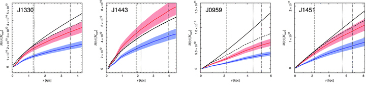
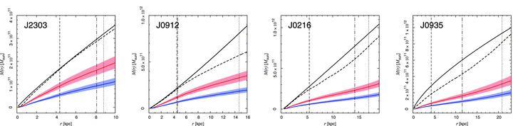
(Credit: Barnabè et al. 2011)
The top row displays the four galaxies with the lowest total mass within the effective radius, while the lower row shows those with the highest mass (mass increases within each row). The solid line is the total enclosed mass profile, while the dashed line is a maximum-bulge fit and the red and blue curves are the stellar-mass contribution derived by two different SPS models (which differ in the assumed initial mass function (IMF) of stars, with the red being a classical Salpeter (1955) IMF and the blue line the more realistic Chabrier (2003) IMF). It is clear that even under the maximum-bulge hypothesis, there has to be a significant amount of dark matter within the radial range probed by the data and when adopting the more realistic SPS stellar masses, most elliptical galaxies require large amounts of dark matter in their inner regions and dark matter indeed dominates the mass budget within the effective radius (the dotted vertical line in each panel). The increasing trend in dark-matter fraction within the effective radius with galaxy mass that is very apparent in the figure above is consistent with the increasing total mass-to-light ratio with velocity dispersion found by Cappellari et al. (2006) that we discussed in Section 17.2 above. Lensing therefore provides further evidence that the tilt of the fundamental plane is caused by differences in the dark-matter fraction or, equivalently total mass-to-light ratio rather than differences in the orbital structure among elliptical galaxies (Bolton et al. 2008b).
A second way to determine the dark matter fraction in the inner regions of elliptical galaxies is to determine the stellar mass and the stellar mass-to-light ratio not using SPS modeling, but instead using microlensing. As we discussed in Chapter 16.2.3, stars in external galaxies are able to produce multiple images for sources that are smaller than \(\approx 0.1\,\mathrm{pc}\). The innermost, unresolved regions of multiply-imaged quasars are small enough for this to be possible. Such multiple images have microarcsecond-scale offsets between the images, which cannot be resolved using any telescope, but the relative movement between the source and the lens stars causes a time-dependent magnification pattern as the source moves in areas of different magnification of the foreground lens (Chang & Refsdal 1979). These microlensing-induced changes to the magnification have typical timescales of one to ten years and they can be observed either by monitoring the flux of multiply-imaged quasars over many years (e.g., Schechter & Wambsganss 2002; Kochanek 2004) or by comparing the magnification at a single time with that predicted by a smooth (i.e., without point-source stars) lens mass model (Schechter et al. 2014; in this case one has to, of course, be quite certain a priori that magnification differences are solely due to microlensing by stars rather than any other non-smoothness in the lensing potential).
Predicting the microlensing magnifications is complicated by the fact that elliptical lenses do not consist of a single star, but instead have up to trillions of stars. Each star has an Einstein radius \(\approx 0.01\,\mathrm{pc}\), which is similar to the typical projected separation between stars in the centers of elliptical galaxies. Therefore, any location in the image plane generally lies within a small number of overlapping Einstein rings and the optical depth to this type of microlensing—the probability that a source is microlensed—is large (Paczynski 1986a). This produces a complex pattern of magnifications as a source moves across the lens and this combined with the fact that the intrinsic quasar flux itself varies in a complex manner means that modeling the time dependence of the observed flux is difficult and must be done numerically (typically using inverse ray tracing, following rays back from the observer to the source, because the lensing equation is simple in this case; Kayser et al. 1986). Because we have no prior information on the relative configuration of stars in the lensing galaxy, fits to observed magnification patterns have to be done by brute force, attempting many different variations of a random star field. An example of the complex magnification pattern near two of the images of the four-image (quad) quasar Q2237+0305 that best fit its observed light curve is displayed in the following figure (each source image moves along the line starting from the open circle):
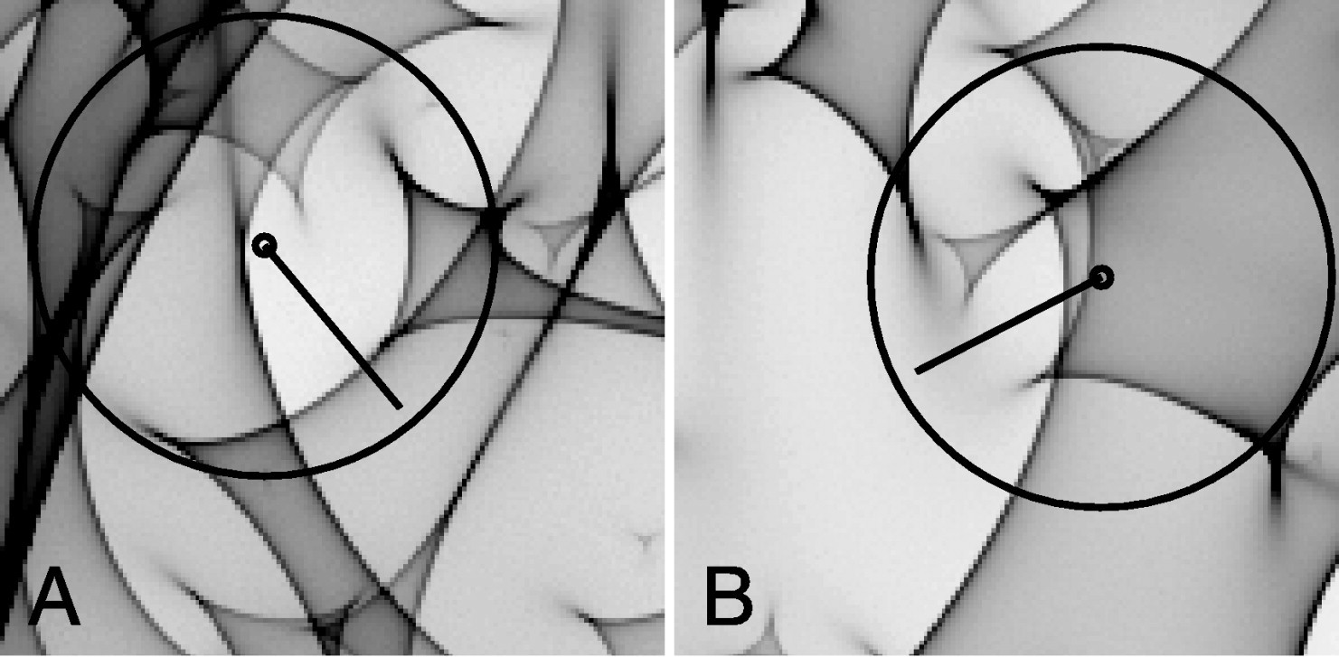
(Credit: Kochanek 2004)
While microlensing by stars in external galaxies is in principle sensitive to the distribution of the masses of the individual stars (Schechter et al. 2004), this dependence in practice is weak and the predicted pattern and frequency of magnification events mainly depends on the total stellar surface density (e.g., Paczynski 1986a; Wyithe et al. 2000; Kochanek 2004). Microlensing is then a great alternative tool to determine the stellar mass and the stellar mass-to-light ratio in elliptical galaxies. For example, Schechter et al. (2014) use the difference between the magnifications of point-like sources predicted by smooth mass models and the observed relative magnifications of X-ray images of multiply-imaged quasars to calibrate mass-to-light ratios obtained using SPS models computed using a Salpeter (1955) IMF. They find that such mass-to-light ratios need to be increased by a factor of 1.23 with a 68% confidence region extending from 0.77 to 2.10. Applying this scaling to the red curve in the figure from Barnabè et al. (2011) above, we see that the stellar contribution may be somewhat larger than estimated there, but it still leaves much dark matter in the inner regions of massive elliptical galaxies. The galaxies used by Schechter et al. (2014) have high velocity dispersions of \(\sigma \gtrsim 200\,\mathrm{km\,s}^{-1}\). A mass-to-light ratio higher than Salpeter means that there are more low-mass stars than in the Salpeter (1955) IMF and such IMFs are therefore known as bottom heavy IMFs. The direct microlensing evidence for an increasingly bottom-heavy IMF in massive ellipticals is consistent with conclusions about the IMF drawn from smooth strong lensing modeling (Treu et al. 2010), dynamical modeling of the ATLAS\(^\mathrm{3D}\) galaxies (Cappellari et al. 2012), and detailed SPS modeling of absorption features in galaxy spectra sensitive to low-mass stars (Conroy & van Dokkum 2012).