
7. Masses of spherical stellar systems
Now that we have covered the theoretical underpinnings of gravitational potentials, orbits, and equilibria of spherical systems, we apply these in this final chapter of the first part to learn about the mass distributions of real stellar systems. Even though most galaxies are far from spherical, we can use the tools we studied in the previous chapters to learn a surprising amount about the overall mass distribution of galaxies and, in particular, about the total dark matter content and its distribution within galaxies.
7.1. The escape velocity near the Sun and the total mass of the Milky Way
We already briefly discussed the escape velocity in the solar neighborhood and its implications for the total mass of the Milky Way in Chapter 4.2. In this section, we take a closer look at how the escape velocity is determined from observational data.
To determine the escape velocity, we can look at a kinematically-unbiased sample of stars—meaning that the stars in the sample were not selected for or against based on their velocity or proper motion—and find a high-velocity cut-off. If a high-velocity cut-off exists, a natural interpretation of that cut-off is that it represents the escape velocity. The cut-off is due to stars with higher velocity never returning to the solar neighborhood. Making this measurement is difficult. By their very nature, stars with velocities near the escape velocity are on orbits with large orbital times which visit the solar neighborhood near their pericenters. Due to conservation of angular momentum, stars spend relatively little time close to their pericenters compared to the rest of their orbits. Therefore, these stars do not spend much time near the Sun for us to observe them. Current samples of stars with velocity measurements near the Sun have hundreds of thousands of stars, yet only a few dozen of these have velocities within \(\approx 200\,\mathrm{km\,s}^{-1}\) of the likely escape velocity that could be used to look for a cut-off. Because of the paucity of data, we need to compare the data to parameterized models of the velocity distribution that include the cut-off at \(v_\mathrm{esc}\).
Stars with high velocities near the Sun spend most of their orbits well into the dark-matter halo rather than near the disk. It therefore makes sense to model them as if they are orbiting in a spherical potential (assuming that the halo is spherical) and we can apply the framework from the previous two chapters. The simplest possible assumption is that the distribution function of high-velocity stars is an ergodic distribution function \(f(\mathcal{E})\) that is only a function of the binding energy \(\mathcal{E}\), similar to the ones that we discussed in Chapter 6.6. As \(\mathcal{E} \rightarrow 0\), ergodic distribution functions with a finite mass approach \(f(\mathcal{E}) \rightarrow 0\) and we can very generally model this approach using a power law of \(\mathcal{E}\). We therefore posit a distribution function of the form
for some \(k\). It is easy to see that this is the case for the Hernquist distribution function that we discussed in Section 6.6.1 and for the King models in Section 6.6.3. Remembering that \(\mathcal{E} = \left(v_\mathrm{esc}^2-v^2\right)/2\) (Equation 6.64), this becomes a probability distribution \(p(v|\vec{x})\) of the magnitude \(v\) of the velocity at a given position \(\vec{x}\) (in this case, the solar neighborhood, which can be considered a single position for this application):
A form similar to this was first proposed by Leonard & Tremaine (1990), but dropping the \((v_\mathrm{esc}+v)^k\) factor when decomposing the right-hand side of Equation \(\eqref{eq-df-vesc-ergodic}\) as \((v_\mathrm{esc}+v)^k\,(v_\mathrm{esc}-v)^k\). The argument made in this paragraph was first made by Kochanek (1996). Because proper motions of stars are difficult to measure (although Gaia is dramatically changing this situation!), data samples that can be used to determine the escape velocity have been typically limited to line-of-sight velocities \(v_\mathrm{los}\) and we therefore need to integrate Equation \(\eqref{eq-df-vesc-ergodic}\) over the tangential velocity; this gives
The distribution function in Equation \(\eqref{eq-df-vesc-ergodic-vlos}\), with parameters \((v_\mathrm{esc},k)\), can be fit to observational data on the line-of-sight velocities \(v_{\mathrm{los},i}\) of a sample of high-velocity stars. Because the velocities of these stars are assumed to be independent draws from \(p(v|\vec{x};v_\mathrm{esc},k)\), the total probability of all observations \(v_{\mathrm{los},i}\) is
Maximizing this probability over \((v_\mathrm{esc},k)\) gives the maximum-likelihood estimate of \((v_\mathrm{esc},k)\).
This type of analysis was performed using the RAVE data by Smith et al. (2007) and later updated by Piffl et al. (2014). The resulting measurement of \(v_\mathrm{esc}\) is \(v_\mathrm{esc} = 530\pm50\,\mathrm{km\,s}^{-1}\). Smith et al. (2007) also tested that the distribution function model of Equation \(\eqref{eq-df-vesc-ergodic}\) is a good model using realistic simulations of the Milky Way’s high-velocity stars. There is good reason to doubt the form of Equation \(\eqref{eq-df-vesc-ergodic}\): As we already discussed, the orbital times of stars with \(v \approx v_\mathrm{esc}\) are very long and the assumption of a steady-state distribution function is therefore suspect; furthermore, the process that populates the \(v \approx v_\mathrm{esc}\) tail of the velocity distribution is uncertain and it does not have to be the case that the distribution function would not reach zero at a non-zero \(\mathcal{E}\). However, Smith et al. (2007) found that the form in Equation \(\eqref{eq-df-vesc-ergodic}\) is a good enough model for the current purposes at least for the simulations.
The escape velocity is a unique constraint on the mass of the Milky Way because, unlike most dynamical constraints, it is sensitive to the cumulative mass outside of the solar circle. As we discussed in Chapter 4.2, unfortunately we have to assume a density distribution for the mass outside of the solar circle, so any determination of the Milky Way’s mass using the escape velocity at the solar circle depends on the assumed density of matter outside of the solar circle. Assuming the cosmologically-motivated NFW profile, the measurement of \(v_\mathrm{esc} = 530\pm50\,\mathrm{km\,s}^{-1}\) gives a total halo mass of \(M \approx 1.3\pm0.4\times10^{12}\,M_\odot\) (Smith et al. 2007; Piffl et al. 2014).
7.2. The Local Group timing argument
One of the first indications that the mass of the Local Group—consisting of the Milky Way, M31, and many smaller galaxies—is much more massive than the total stellar masses of all of its constituents came from the Local Group timing argument. This argument was first made by Kahn & Woltjer (1959). The crux of the argument is the following: Because the Milky Way and M31 are by far the largest galaxies in the Local Group, it makes sense to approximate the mass of the Local Group as being all contained in the Milky Way and M31. A simple way to model their dynamics then is to assume that both large galaxies are point masses that have been orbiting each other since the Big Bang. At the Big Bang, both (proto)-galaxies were at the same position \(r=0\) and were launched on a zero-angular momentum orbit to where we see them today. From the age of the Universe and the present-day relative velocity and distance between the Milky Way and M31 we can solve for the orbit and the total mass of the system. We can solve for the mass from these three observables, because the orbit is characterized by two parameters only: the initial radial velocity (because the initial separation and the angular momentum are zero) and the current orbital phase. Because a collision between the galaxies would cause them to merge, we can assume that the orbit is still in its first radial period and \(T_r > t_\mathrm{H}\), with \(t_\mathrm{H} = 13.7\,\mathrm{Gyr}\) the age of the Universe.
The orbit of two point masses can be solved by going to the center-of-mass reference frame. If the Milky Way’s mass is \(M_\mathrm{MW}\) and M31’s mass is \(M_\mathrm{M31}\), then the total mass is \(M = M_\mathrm{MW} + M_\mathrm{M31}\), the reduced mass is \(\mu = M_\mathrm{MW}\,M_\mathrm{M31}/(M_\mathrm{MW}+M_\mathrm{M31})\); the Milky Way’s position is \(\vec{x}_\mathrm{MW}\) and M31’s position is \(\vec{x}_\mathrm{M31}\) and the center of mass is therefore at a vector \(\vec{X} = (M_\mathrm{MW}\,\vec{x}_\mathrm{MW} + M_\mathrm{M31}\,\vec{x}_\mathrm{M31})/M\). Because of the conservation of momentum in this system, the center of mass is fixed. It is then straightforward to show that the time dependence of the separation vector (or displacement vector) \(\vec{r} = \vec{x}_\mathrm{M31}-\vec{x}_\mathrm{MW}\) follows the same orbit as a particle with a mass equal to \(\mu\) in a fixed point-mass potential with mass \(M\), with the center of mass \(\vec{X}\) as the origin. This is the orbit that we solved in Chapter 5.2.2.
Rather than directly solving Kepler’s equation for the mass \(M\) implied by the observations, let’s use the conservation of energy and angular momentum to make a simple estimate. The energy in a point-mass potential is given in terms of the semi-major axis \(a\) by Equation (5.54), and energy conservation during the orbit therefore means that
where \(r = |\vec{r}|\), the magnitude of the separation vector and \(v = |\vec{v}|\) is the magnitude of the relative velocity. Re-writing this as follows gives the relative velocity in terms of the mass and displacement
We can use Kepler’s third law (Equation 5.51)—a statement of the conservation of angular momentum—to substitute the period \(T_r\) for the semi-major axis \(a\) in this equation and derive a relation between the relative velocity, the period, and the separation
We can write this as a cubic equation for \(x = G\,M\)
The current separation between the Milky Way and M31 is \(r \approx 740\,\mathrm{kpc}\) and the current relative velocity is \(v \approx -125\,\mathrm{km\,s}^{-1}\) (where we’ve included the sign to indicate that M31 is currently approaching the Milky Way). To apply Equation \(\eqref{eq-lgtiming-deriv-2}\), we need \(T_r\). Let’s estimate \(T_r\) by approximating the time until the next collision as \(t_c = -r/v\) and adding this to the age of the Universe to estimate \(T_r\): \(T_r \approx t_\mathrm{H}-r/v\). Then we can solve the cubic equation. Here’s the code that does this
[7]:
import numpy
import astropy.constants as apyconst
import astropy.units as u
# Observables
r= 740.*u.kpc
v= -125.*u.km/u.s
tH= 13.7*u.Gyr
# Estimate T_r
Tr= tH-r/v
# We will rewrite the cubic equation in terms of M12 = M/(10^12 Msun)
# so we need a tG = G x 10^12 Msun
tG= apyconst.G*10.**12.*u.Msun
sol= numpy.roots([-8.*(tG**3./r**3.).to((u.km/u.s)**6).value,
                  ((12.*v**2./r**2.+4*numpy.pi**2./Tr**2.)*tG**2.)\
                          .to((u.km/u.s)**6).value,
                  -6.*(v**4./r*tG).to((u.km/u.s)**6).value,
                  (v**6.).to((u.km/u.s)**6).value])
sol= sol[numpy.isreal(sol)]
print("The approximate LG timing mass is %.2f x 10^12 Msun" % sol.real)
The approximate LG timing mass is 4.00 x 10^12 Msun
Thus, we see that the mass for the Local Group implied is approximately \(M = M_\mathrm{MW}+M_\mathrm{M31} = 4\times10^{12}\,M_\odot\). The radial period \(T_r\) will in reality be somewhat smaller than the rough estimate that we used and it is easy to check (by running the above code for different \(T_r\)) that a smaller \(T_r\) leads to a larger mass. The approximate timing mass that we have derived here is therefore a lower limit. An upper limit can be obtained by setting \(T_r = t_\mathrm{H}\), which gives \(M = 5.5\times 10^{12}\,M_\odot\), so without doing any complicated Keplerian orbit modeling, we find that
Li & White (2008) demonstrated, by applying the timing argument to groups with two large galaxies in the Millenium simulation, that the timing argument has an uncertainty of a factor of two, larger than the range that we get from our simple derivation above.
The full, exact solution that solves for \(T_r\) by directly solving for the orbit is left as an exercise. That solution gives \(T_r = 16.6\,\mathrm{Gyr}\). If you plug this into the code above, you find that this implies \(M = 4.6\times10^{12}\,M_\odot\).
The mass for the Local Group implied by the timing argument is at least an order of magnitude larger than the total mass in stars in all Local Group galaxies. The timing argument therefore provided an early indication that galaxies like the Milky Way are surrounded by extended, massive halos of dark matter.
7.3. The mass of the Milky Way’s dark matter halo
Given that we know from, e.g., the escape velocity near the Sun and from the Local Group timing argument that the Milky Way disk must be surrounded by a massive halo of dark matter, we would like to find out more about the mass profile of this dark-matter halo. Because the disk only extends out to about 15 kpc from the center, any dynamical analysis that wants to determine the mass profile at larger distances must use non-disk tracers, such as globular clusters (see Chapter 6.2) or stars orbiting in the stellar halo. The simplest assumption is that the dark-matter halo is spherical and that it dominates the mass outside of the disk, such that the total potential is also approximately spherical. Then we can use the spherical Jeans equation.
We derived the spherical Jeans equation in Chapter 6.4. Let’s write the spherical Jeans equation (6.54) in terms of the circular velocity rather than the enclosed mass
Therefore, to observationally determine the circular velocity curve \(v_c(r)\) using the spherical Jeans equation in the Milky Way, we need to measure \(\nu(r)\), \(\sigma_r(r)\), and \(\beta(r)\) of the tracer population that we are using. It is possible to measure \(\nu(r)\) for large photometric samples of halo stars (e.g., Bell et al. 2008). Because we do not (yet!) have large data samples with three-dimensional velocities, determining \(\sigma_r(r)\) and especially \(\beta(r)\) is more difficult. At large \(r\) (\(r \gg R_0\), the solar radius), \(\sigma_r(r)\) is approximately equal to \(\sigma_\mathrm{los}(r)\), because to a good approximation the Sun is sitting at the center of the Galaxy in this case and therefore \(v_\mathrm{los} \approx v_r\). For the same reason, \(\beta(r)\) can only be measured using tangential velocities (i.e., proper motions).
Xue et al. (2008) presented a sample of \(\approx 2,400\) blue-horizontal branch (BHB) stars from SDSS with well-measured distances and \(v_\mathrm{los}\). They analyzed these primarily by comparing them to a cosmological simulation, but also applied a simple Jeans analysis that agreed with the more complex analysis. For the SDSS survey volume, they found that \(\sigma_r(r) \approx \sigma_\mathrm{los}(r)\) to good accuracy. From the large sample of BHB stars, they could precisely determine \(\sigma_\mathrm{los}\) and found it to be slowly declining with radius as
They combined this with \(\nu(r) \propto r^{-3.5}\) in Equation \(\eqref{eq-spher-jeans-anisotropy-vc}\) to determine \(v_c(r)\) using \(\beta = 0\) as the simplest, isotropic assumption and using \(\beta = 0.37\), as informed by numerical simulations. Before discussing the results in more detail, we note that both choices lead to \(v_c \approx 200\,\mathrm{km\,s}^{-1}\) and we estimate the uncertainty in \(v_c\) coming from our lack of knowledge of \(\beta\) (a manifestation of the mass–anisotropy degeneracy). From Equation \(\eqref{eq-spher-jeans-anisotropy-vc}\) we have that
using \(\sigma_r \approx 111\,\mathrm{km\,s}^{-1}\) and \(v_c \approx 200\,\mathrm{km\,s}^{-1}\).
The rotation curve \(v_c(r)\) derived from the Jeans equation in the form \eqref{eq-spher-jeans-anisotropy-vc} by Xue et al. (2008) is shown in the following figure:
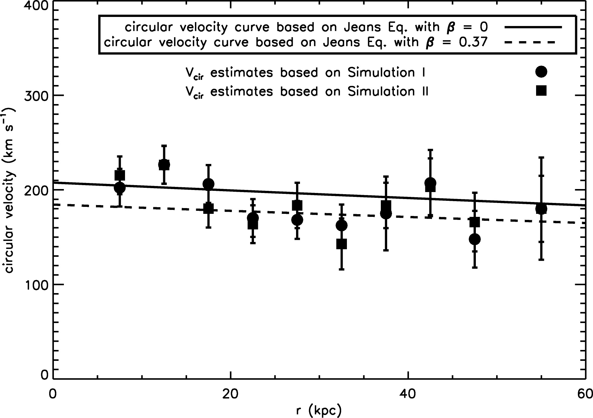
(Credit: Xue et al. 2008)
The solid line shows the derived rotation curve when \(\beta = 0\), while the dashed line uses \(\beta = 0.37\). From Equation \(\eqref{eq-Xue-beta-depend}\), we expect \(\Delta v_c \approx -23\,\mathrm{km\,s}^{-1}\) and approximately constant across the radial range, which agrees with this figure. Because the uncertainty in \(\beta\) mostly gives rise to a constant offset (unless \(\beta(r)\) has a strong radial variation), the slope of \(v_c(r)\) is robust. The best-fit circular velocity profile is declining, which implies that the mass density declines faster than \(r^{-2}\), as expected for dark-matter halos from cosmological simulations.
Equation \(\eqref{eq-Xue-beta-depend}\) makes it clear that the anisotropy parameter \(\beta\) has a large effect on the rotation curve that we derive from the halo BHB kinematics. Much effort is therefore going towards determining \(\beta\). For example, Deason et al. (2013) used Hubble-Space-Telescope proper motions for a few halo stars to determine \(\beta = 0.0^{+0.2}_{-0.4}\) around \(r = 25\,\mathrm{kpc}\), indicating that the halo is approximately isotropic in that range.
Because \(v_c^2 = G\,M(<r)/r\), we can model the data in the above figure with a mass model for the Milky Way. Xue et al. (2008) do this with a simple disk+bulge+halo model, where the disk is modeled as a spherical potential with an exponential density (what could be called the “spherical-cow disk model”). From this they find \(M(<60\,\mathrm{kpc}) = 4.0\pm0.7\times10^{11}\,M_\odot\) and a total mass \(M_\mathrm{MW} = 1.0\pm0.3\times10^{12}\,M_\odot\). This is similar to the total halo mass found from the local escape velocity in Section 7.1 above.
7.4. The masses of dwarf spheroidal galaxies using the Jeans equation
Dwarf spheroidal galaxies (dSphs) are low-luminosity, low-mass galaxies that are the smallest galaxies that form in the Universe. Galaxy formation and evolution in such galaxies is very different from that in large galaxies like the Milky Way. dSphs therefore present a unique laboratory for finding the threshold of galaxy formation: how do stars form in low-mass galaxies, how do they enrich their interstellar medium, what happens to these galaxies as they accrete onto larger galaxies, and, importantly, what are their dark-matter distributions?
dSphs are commonly found around the Milky Way, where we can see the lowest luminosity galaxies that are too dim and too low in surface brightness to be seen around external galaxies. Determining the masses and mass-to-light ratios of these galaxies is important for different reasons: (i) the ratio of stellar-to-dark-halo mass in these galaxies tells us about the efficiency of star formation in low-mass galaxies, (ii) because the mass-to-light ratios of these galaxies appear to be high they are dominated by dark matter at all radii and can therefore provide a pristine look at the dark-matter distribution in galaxies (although whether this is really true is still under debate), (iii) if dark matter would happen to annihilate, these galaxies make for good targets to see the products of such annihilation (e.g., Springel et al. 2008b), and (iv) for other reasons.
Around the Milky Way, we have so-called classical dwarfs spheroidals like Draco, Fornax, and Sculptor and ultra-faint dwarf spheroidals. The former have been known for decades and they are relatively massive with stellar masses of about \(10^6\) to \(10^7\,M_\odot\). The latter have very low surface brightness and low stellar masses; they were only discovered using wide-field multi-band surveys like SDSS (e.g., Willman et al. 2005, Belokurov et al. 2007) and DES (e.g., Bechtol et al. 2015) that allow slight stellar overdensities in the stellar halo to be detected. For the classical dSphs, large spectroscopic data sets of line-of-sight velocities have been created, for example, the data set from Walker et al. (2009a), represented in the following figure:
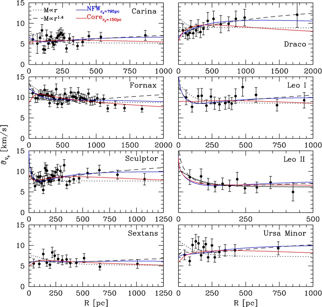
(Credit: Walker et al. 2009b)
These data can be used to measure the masses and mass profiles of dSphs using dynamical modeling. Measurements of the surface-density profile \(\Sigma(R)\) are available for these dSphs from direct star counts. These can be deprojected to three-dimensional density profiles \(\nu(r)\) for use in, e.g., the Jeans equation. One way of doing this is by fitting the surface-density profile with a simple form, such as a Plummer profile (see Chapter 3.4.3) , which provides a good fit to the observed surface-density profiles of dSphs. The two-dimensional projection of the Plummer profile is
for a total stellar mass \(M_*\) and a two-dimensional half-mass radius \(R_e\) (that is, the cylindrical radius that contains half of the stellar mass). Once the surface-density profile has been fit with a Plummer profile, the three-dimensional density of this profile can be used. Another option is to use the fact that if we assume that the underlying profile is spherically symmetric, the surface density \(\Sigma(R)\) is related to the three-dimensional density \(\nu(r)\) as follows
This is an Abel integral equation, which can be inverted to
Thus, we can directly recover the three-dimensional density \(\nu(r)\) from a measurement of the projected surface density \(\Sigma(R)\).
The second ingredient for the spherical Jeans equation is \(\sigma^2_r(r)\). However, the measurements of the line-of-sight velocities in dSphs give \(\sigma_\mathrm{los}^2\). While in the Milky Way analysis \(\sigma_r \approx \sigma_\mathrm{los}\), this is only due to our position close to the center of the Milky Way. For external systems, we cannot set \(\sigma_r = \sigma_\mathrm{los}\). What we need to do is compute \(\sigma_\mathrm{los}(R)\) from \([\Sigma(R),\nu(r),\sigma_r(r),\beta]\). Binney & Mamon (1982) demonstrated that \(\sigma_\mathrm{los}(R)\) is given by
Assuming some form of \(\beta(r)\), we can substitute \(\nu(r)\,\sigma_r^2\) obtained from the integrated Jeans equation (equation 6.56 for constant \(\beta\) or equation 6.59 for general \(\beta(r)\) profiles) in this equation and predict \(\sigma_\mathrm{los}\) for a given \([\nu(r),\Sigma(R)]\) pair (related through Equation \([\ref{eq-3ddens-2ddens}]\)), an assumed mass profile \(M(<r)\), and the anisotropy \(\beta(r)\). This predicted \(\sigma_\mathrm{los}\) can then be compared to the data and the (parameters of) the mass profile \(M(<r)\) can be adjusted to give the best fit.
This analysis was performed by, e.g., Walker et al. (2009b) using the \(\sigma_\mathrm{los}\) data above to determine the mass profiles of 8 classical dwarf spheroidals. They found that they were in particular able to robustly determine the mass within \(R_e\) (which they denote as \(r_\mathrm{half}\)), largely independent of the value of \(\beta\). See the following figure for \(M(<R_e)\) and the average density within \(R_e\):
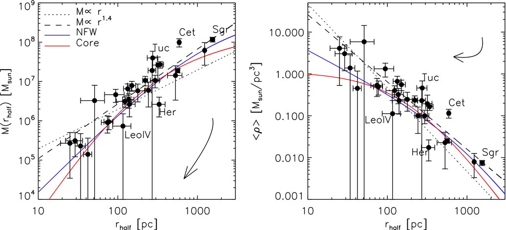
(Credit: Walker et al. 2009b)
These results imply that the dSphs are embedded in massive dark-matter halos, with mass-to-light ratios of 10 to 100. The Jeans analysis of these data, however, is not sensitive to the inner profile of the dark-matter halo and in particular cannot easily distinguish between a cored (\(\rho \propto\mathrm{constant}\)) or a cuspy (\(\rho \propto r^{-1}\)) profile. This is an important question, as the prediction from the reigning cold dark-matter paradigm is that the inner profiles should be cuspy (although the exact prediction depends on uncertain baryonic feedback effects).
7.5. The Wolf mass estimator
Before discussing how we can distinguish between a cored and a cuspy inner dark-matter profile using Jeans analyses of the dSph data, let’s understand one key result mentioned above better: that the enclosed mass at the half-mass radius is robust against variations in the assumed anisotropy \(\beta\). It turns out that we can construct a very robust mass estimator for spherical systems using this result. We present here a slightly simplified derivation of the resulting mass estimator first derived by Wolf et al. (2010).
We start by re-writing Equation \(\eqref{eq-surfdens-siglos-jeans}\) in the form \(\Sigma(R)\,\sigma_\mathrm{los}^2(R) = \int_{R^2}^\infty\mathrm{d}r^2\,\frac{1}{\sqrt{r^2-R^2}}\,f(r^2)\) to make it amenable to inversion through an Abel transform. The result of a somewhat tedious calculation is
This can be inverted through an Abel transform to give
The right-hand side of this equation depends solely on observable quantities, the two-dimensional projected stellar surface density \(\Sigma(R)\) and the line-of-sight velocity dispersion \(\sigma_\mathrm{los}\). The left-hand side of the equation therefore also needs to be independent of the underlying model. That is, the unknown functions need to combine to give a model-free value to match the right-hand side. The three-dimensional density \(\nu(r)\) is directly related to \(\Sigma(R)\) through Equation \(\eqref{eq-3ddens-2ddens}\), and the model functions that can vary in Equation \(\eqref{eq-wolf-nusig-abeltransformed}\) are therefore only \(\sigma_r(r)\) and \(\beta(r)\). Assuming that an isotropic solution exists, we can equate the left-hand side for non-zero \(\beta\) with that for zero \(\beta\)
where we have written \(\sigma_r(r)\) as \(\sigma_r(r;\beta=0)\) or \(\sigma_r(r;\beta)\) to indicate that the necessary radial dispersion to match the observable right-hand side of Equation \(\eqref{eq-wolf-nusig-abeltransformed}\) depends on \(\beta\). Then we take the derivative of Equation \(\eqref{eq-wolf-nusig-diffbeta}\) with respect to \(\ln r\)
and use the spherical Jeans Equation (6.54) to write this equation in terms of the mass derived for different \(\beta\)
We can then solve for a radius \(r_\mathrm{eq}\) where the difference in the mass estimated using different \(\beta\) is zero. Assuming that \(\beta \neq 0\) this means that we need
For realistic systems, the stellar density will vary over orders of magnitude, while changes in \(\beta\) are \(\mathcal{O}(1)\), and we can therefore set \(\mathrm{d} \ln \beta/\mathrm{d} \ln r \approx 0\). As we saw above for the dSphs, for many observed systems we have that \(\sigma_\mathrm{los}(R) \approx \mathrm{constant}\), which is difficult to achieve with a strongly varying \(\sigma_r(r)\), so we can also set \(\mathrm{d} \ln \sigma_r^2/\mathrm{d} \ln r \approx 0\) (see Wolf et al. 2010 for more detailed arguments for this assumption). Equation \(\eqref{eq-wolf-solve-req}\) then becomes
This means that the radius where the enclosed mass does not depend strongly on \(\beta\) is that radius \(r_3\) where the logarithmic slope of the density profile is \(-3\).
To obtain the mass enclosed within \(r_3\), we go back to Equation \(\eqref{eq-wolf-nusig-abeltransformed}\), set \(\beta=0\) (because the mass does not depend on \(\beta\)) and take the derivative of both sides of the equation with respect to \(\ln r\)
where both sides are evaluated at \(r_\mathrm{eq}\). For the case where \(\sigma_\mathrm{los} \approx \mathrm{constant}\), we can bring \(\sigma_\mathrm{los}^2\) outside of the integral and use Equation \(\eqref{eq-3ddens-2ddens}\) to replace the integral with \(\nu(r)\)
Using the spherical Jeans Equation (6.54), this becomes
Using Equation \(\eqref{eq-wolf-req-3}\), we find
Because \(r_3\) is defined by a property of the deprojected stellar density profile it is not a directly observable quantity. For most realistic stellar density profiles (e.g., the Plummer and King profiles, and common Sérsic profiles [see Equation 2.2]), it happens to be the case that \(r_3 \approx r_{1/2}\), with \(r_{1/2}\) the three-dimensional radius that contains half of the mass (the half-mass radius). For the same profiles, it is also the case that \(r_{1/2} \approx 4 R_e/3\), with \(R_e\) the two-dimensional radius that contains half of the mass. In terms of these we have the final Wolf mass estimator
When using this estimator, it is important to keep clear about the meaning of the half-mass radius. This is the radius that contains half of the mass in the tracer population. If most of the mass is in a different component, e.g., dark matter, then the half-mass radius of all of the mass can be much larger than the half-mass radius of the tracer population.
To see in practice how the enclosed mass near the half-mass radius is insensitive to the assumed anisotropy, we can model the line-of-sight velocity dispersion for the Carina dSphs from Walker et al. (2009b) that was shown above. For simplicity, we take these data to be that \(\sigma_\mathrm{los} = 6\,\mathrm{km\,s}^{-1}\) at five radii from \(r=50\,\mathrm{pc}\) to \(950\,\mathrm{pc}\). We use the Plummer profile for the stars given by Walker et al. (2009b), which has \(M = 3\times2.4\times 10^5\,M_\odot\)—assuming a mass-to-light ratio of 3—and \(b = 137\,\mathrm{pc}\) (for a Plummer profile \(b = R_e\), the two-dimensional half-mass radius). We then apply the spherical Jeans equation for different values of \(\beta\), fitting the gravitational potential as a general two-power density model from Chapter 3.4.6 with four free parameters: the amplitude, scale radius, and inner- and outer slopes of \(\mathrm{d} \ln \rho / \mathrm{d} r\). This fit is done for four values of \(\beta\) in the following code (we split the fits into two cells, because each fit takes about 4 minutes):
[252]:
from galpy.potential import PlummerPotential, TwoPowerSphericalPotential
from galpy.df import jeans
from scipy import optimize
Re= 137.*u.pc
stellar_pot= PlummerPotential(amp=3.*2.4*1e5*u.Msun,b=Re)
def setup_mass_profile(params):
    mass_pot= TwoPowerSphericalPotential(amp=10.**params[0]*u.Msun,
                                         a=10**params[1]*u.pc,
                                         alpha=params[2],
                                         beta=params[3])
    mass_pot.turn_physical_off()
    return mass_pot
def predict_sigmalos(rs,mass_pot,beta):
    return numpy.array([jeans.sigmalos(mass_pot,r,
                                       dens=lambda r: stellar_pot.dens(r,0,
                                                                       use_physical=False),
                                       surfdens=lambda R: stellar_pot.surfdens(R,\
                                                        1000,use_physical=False),
                                       beta=beta)*220.
                        for r in rs])
def fit_mass_profile(beta):
    def sigmalos_chi2(params):
        # Check that p[2] = inner slope of the mass density is >0 and <3
        if params[2] < 0 or params[2] >= 3: return numpy.inf
        if params[3] <=  2: return numpy.inf
        if 10**params[1] < 50. or 10**params[1] > 3000.: return numpy.inf
        # Initialize mass model
        mass_pot= setup_mass_profile(params)
        # Predict sigma_los(r) at 5 different radii from 100 to 1000 pc
        sigmalos_pred= predict_sigmalos(numpy.linspace(50.,950.,5)*u.pc,
                                        mass_pot,beta)
        return numpy.sum((sigmalos_pred-6.)**2.)
    # We only do a rough fit with 50 evaluations to get a relatively quick result
    bestfit= optimize.minimize(sigmalos_chi2,[7.,2.3,1,3],method='powell',
                               options={'xtol':0.05,'ftol':0.1,
                                        'maxiter':10,'maxfev':50}).x
    return setup_mass_profile(bestfit)
betas= [0.5,0,-0.5,-3.0]
bf_mass_pots= []
for beta in betas[:2]:
    bf_mass_pots.append(fit_mass_profile(beta))
[253]:
for beta in betas[2:]:
    bf_mass_pots.append(fit_mass_profile(beta))
We then plot the resulting \(\sigma_\mathrm{los}(r)\) to demonstrate that all four values of \(\beta\) are able to produce a flat \(\sigma_\mathrm{los}(r)\) over Carina’s inner kpc. We also plot the resulting best-fit enclosed-mass profile for the four fits:
[107]:
figsize(12,5)
subplot(1,3,1)
for ii,beta in enumerate(betas):
    prs= numpy.linspace(50.,1000.,11)*u.pc
    plot(prs.to_value(u.pc),
         predict_sigmalos(prs,bf_mass_pots[ii],beta),
        label=r'$\beta = {:+.1f}$'.format(beta))
xlabel(r'$r\,(\mathrm{pc})$')
ylabel(r'$\sigma_\mathrm{los}\,(\mathrm{km\,s}^{-1})$')
ylim(0.,15.)
legend(frameon=False,fontsize=18.)
subplot(1,3,2)
for ii,beta in enumerate(betas):
    prs= numpy.linspace(0.01,1.,61)*u.kpc
    semilogy(prs.to_value(u.pc),
             [bf_mass_pots[ii].mass(r,ro=8.,vo=220.).to_value(u.Msun)
              for r in prs],
            label=r'$\beta = {:+.1f}$'.format(beta))
semilogy(prs.to_value(u.pc),
             [stellar_pot.mass(r,ro=8.,vo=220.).to_value(u.Msun) for r in prs],
        ls=':',color='k')
axvline(4.*Re.to_value(u.pc)/3.,ls='--',color='0.7',lw=2.,zorder=0)
import astropy.constants as apyconst
axhline((4.*(6.*u.km/u.s)**2*Re/apyconst.G).to_value(u.Msun),
        ls='--',color='0.7',lw=2.,zorder=0)
text(225.,5e7,r'$r_{1/2}$',fontsize=18.,horizontalalignment='left')
text(600.,4e5,r'$\mathrm{stars}$',fontsize=18.,horizontalalignment='left')
xlabel(r'$r\,(\mathrm{pc})$')
ylabel(r'$M(<r)/M_\odot$')
ylim(1e5,1e8)
legend(frameon=True,fontsize=18.,facecolor='w',edgecolor='None')
subplot(1,3,3)
for ii,beta in enumerate(betas):
    prs= numpy.linspace(0.01,1.,61)*u.kpc
    plot(prs.to_value(u.pc),
             [bf_mass_pots[ii].mass(r,ro=8.,vo=220.).to_value(u.Msun)
              /bf_mass_pots[1].mass(r,ro=8.,vo=220.).to_value(u.Msun)
              for r in prs],
         label=r'$\beta = {:+.1f}$'.format(beta))
axvline(4.*Re.to_value(u.pc)/3.,ls='--',color='0.7',lw=2.,zorder=0)
xlabel(r'$r\,(\mathrm{pc})$')
ylabel(r'$M(<r;\beta)/M(<r;\beta=0)$')
tight_layout();
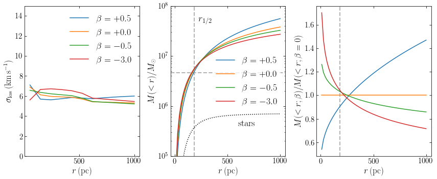
Because the enclosed mass spans a few orders of magnitude over the inner kpc, we also display the enclosed-mass profile relative to that obtained for \(\beta = 0\) in the right-most panel. From that panel, it becomes clear that all four values of \(\beta\) do indeed produce a similar value for the enclosed mass near the half-mass radius (although in this case, the value where all anisotropies agree is a little higher still). We also show the contribution to the enclosed-mass profile from the stars, which demonstrates that Carina, like all dSphs, is indeed a very dark-matter dominated system, with \(M/L \approx 150\) within 1 kpc.
7.6. Ultra-diffuse galaxies and Dragonfly 44
We can use the Wolf estimator to learn about the nature of a new population of galaxies that has recently garnered much interest: ultra-diffuse galaxies (UDGs). These are galaxies that have a very low surface brightness and low luminosity, comparable to that of the dwarf spheroidals that we discussed earlier in this chapter, but that have sizes that are an order of magnitude larger, making them of similar size to large galaxies like the Milky Way, even though they contain orders of magnitude fewer stars. These galaxies have primarily been found in galaxy clusters, such as the Coma cluster (van Dokkum et al. 2015; Koda et al. 2015).
How these UDGs form is a bit of a mystery and one important ingredient in the puzzle is what their total masses are (stars, gas, and dark matter). This can shed light on the type of potential well that the stars in these galaxies formed in and can help understand how these galaxies are able to survive in a cluster environment, where small galaxies are likely to be tidally pulled apart. Because of their low surface brightness, obtaining velocity dispersions for these systems is difficult, but a few groups have done so and we can interpret these measurements using the Wolf estimator to determine the total mass of some of the UDGs. Before embarking on this, we should note that the Wolf estimator (and all of the mass modeling approaches that we have discussed so far) assume dynamical equilibrium for the tracer stars, which may not be a good assumption if the UDGs are strongly tidally interacting with their host clusters. But we will boldly move ahead under the assumption of dynamical equilibrium and see whether a consistent picture emerges.
A first measurement of the velocity dispersion of a set of tracers in a UDG was presented by Beasley et al. (2016). Here is an image of the ultra-diffuse galaxy VCC 1287 in the Virgo cluster:
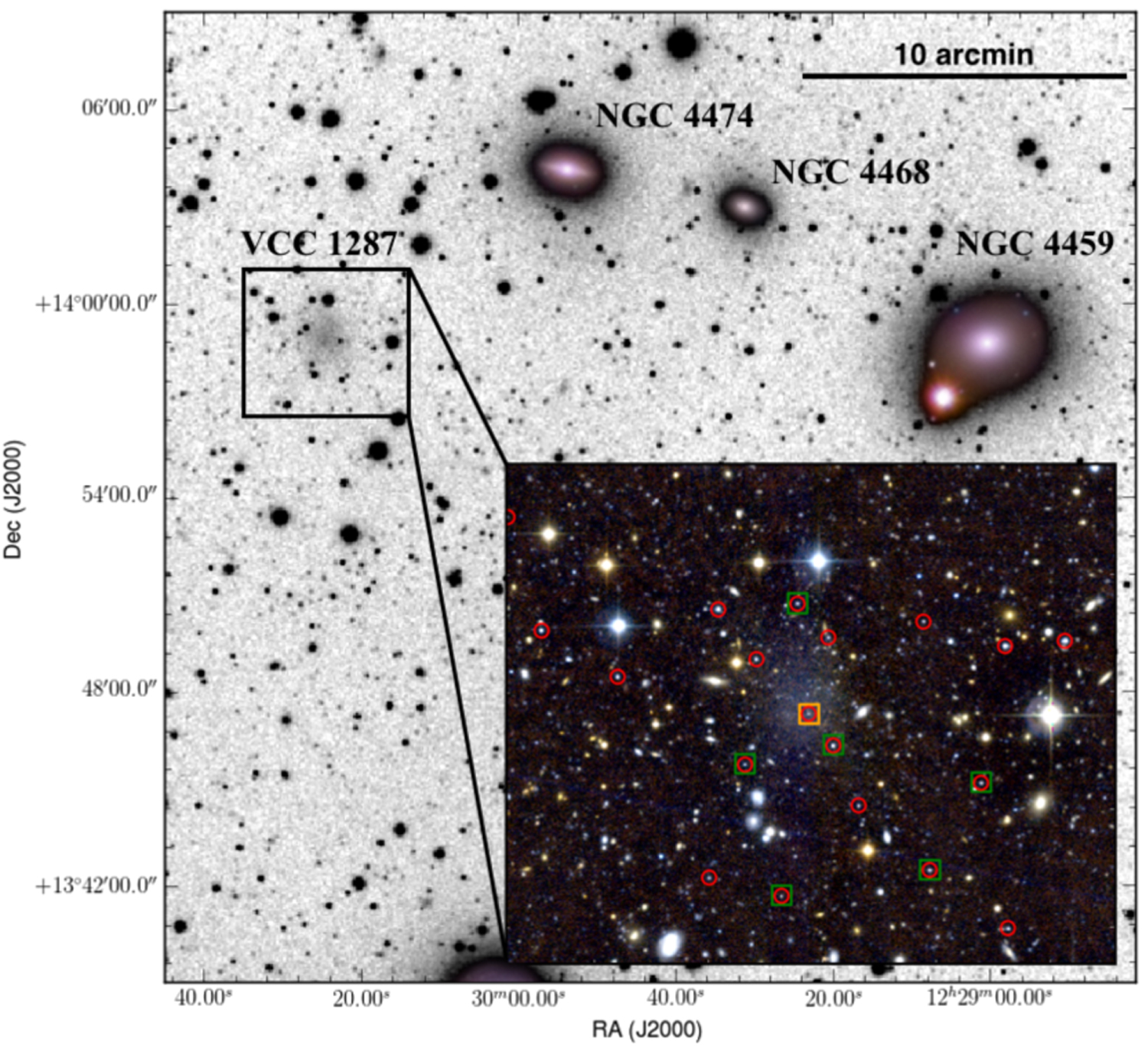
(Credit: Beasley et al. 2016)
The authors of this work identified candidate globular clusters associated with VCC 1287 and measured their line-of-sight velocities. They found seven globular clusters that are likely associated with VCC 1287, which are indicated by the green and orange boxes in the image above. For these clusters, they measure a line-of-sight velocity dispersion of \(\sigma_\mathrm{los} = 33^{+16}_{-10}\,\mathrm{km\,s}^{-1}\). The half-mass radius of this sytem is approximately \(R_e \approx 2.4\,\mathrm{kpc}\), and using the Wolf estimator from Equation \(\eqref{eq-wolf-re}\) gives
[9]:
# Function that gives Wolf estimate
import astropy.constants as apyconst
def wolf_estimator_re(sig_los,Re):
    return (4.*sig_los**2.*Re/apyconst.G).to(10**10*u.Msun)
# Apply to VCC 1287
sig_los= 33.*u.km/u.s
sig_los_up= 49.*u.km/u.s
sig_los_down= 23.*u.km/u.s
Re= 2.4*u.kpc
print("""The mass of VCC 1287 from the Wolf estimator is {0:.2f}
         with uncertainty +{1:.2f} and -{2:.2f}"""\
      .format(wolf_estimator_re(sig_los,Re),
              (wolf_estimator_re(sig_los_up,Re)
               -wolf_estimator_re(sig_los,Re)),
             (wolf_estimator_re(sig_los,Re)
               -wolf_estimator_re(sig_los_down,Re))))
The mass of VCC 1287 from the Wolf estimator is 0.24 1e+10 solMass
         with uncertainty +0.29 1e+10 solMass and -0.12 1e+10 solMass
Combined with the total stellar luminosity, this gives a mass-to-light ratio \(M/L \approx 100\) within \(R_e = 2.4\,\mathrm{kpc}\). The half-mass radius is close to the center and if these UDGs are embedded in dark-matter halos—as certainly seems to be the case from the large \(M/L\)—then these halos extend to much larger radii. By extrapolating the enclosed mass at \(1\,R_e\) to an estimate of the total halo mass, Beasley et al. (2016) find a total dark-matter mass of \(\approx 10^{11}\,M_\odot\). This makes VCC 1287 a very large galaxy indeed. But the uncertainty in the mass is quite large, because of the large uncertainty in \(\sigma_\mathrm{los}\).
Dragonfly 44 is another ultra-diffuse galaxy for which the line-of-sight velocity dispersion was measured. van Dokkum et al. (2016) obtained deep Keck spectroscopy of Dragonfly 44 to measure the stellar velocity dispersion. Dragonfly 44 is a UDG in the Coma cluster:
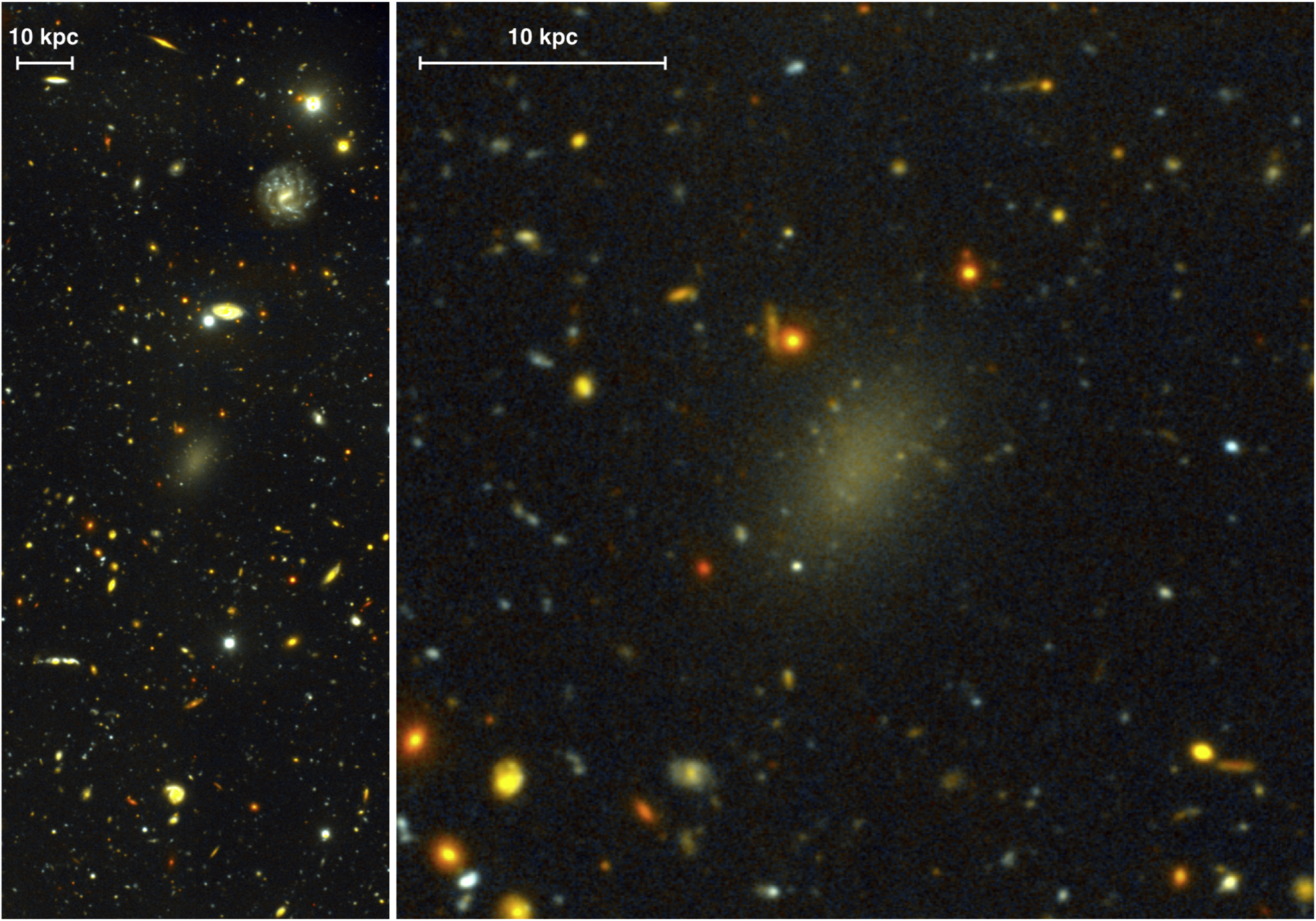
(Credit: van Dokkum et al. 2016)
They obtained a velocity dispersion of \(\sigma_\mathrm{los} = 47^{+8}_{-6}\,\mathrm{km\,s}^{-1}\), with no evidence of a radial trend in \(\sigma_\mathrm{los}\). The assumptions underlying the Wolf estimator are therefore satisfied and we can combined \(\sigma_\mathrm{los}\) with the measured half-mass radius \(R_e = 3.5\,\mathrm{kpc}\) to give the mass enclosed by the half-mass radius
[11]:
# Apply to Dragonfly 44
sig_los= 47.*u.km/u.s
sig_los_up= 55.*u.km/u.s
sig_los_down= 41*u.km/u.s
Re= 3.5*u.kpc
print("""The mass of Dragonfly 44 from the Wolf estimator is {0:.2f}
         with uncertainty +{1:.2f} and -{2:.2f}"""\
      .format(wolf_estimator_re(sig_los,Re),
              (wolf_estimator_re(sig_los_up,Re)
               -wolf_estimator_re(sig_los,Re)),
             (wolf_estimator_re(sig_los,Re)
               -wolf_estimator_re(sig_los_down,Re))))
The mass of Dragonfly 44 from the Wolf estimator is 0.72 1e+10 solMass
         with uncertainty +0.27 1e+10 solMass and -0.17 1e+10 solMass
The mass-to-light ratio within the half-mass radius is \(M/L \approx 50\), corresponding to a dark matter fraction of \(\approx 98\,\%\) within \(r_{1/2} \approx 1.33\,R_e = 4.6\,\mathrm{kpc}\). Extrapolating the mass to the total mass of the dark-matter halo gives a mass of \(\approx 10^{12}\,M_\odot\), similar to the dark-matter mass in the Milky Way (see above). We showed the mass profile of the Milky Way in Chapter 2.2.1: at \(r\approx 3.5\,\mathrm{kpc}\), the dark-matter fraction in the Milky Way is only \(\approx30\,\%\) and the mass is dominated by stars. Dragonfly is therefore a very different galaxy from the Milky Way: even though they both have about the same total mass in dark matter and therefore presumably live in similar potential wells, Dragonfly 44 only managed to produce about 1% of the stars in the Milky Way and star formation must therefore have been very inefficient in Dragonfly 44 compared to the Milky Way! Of course, they do live in very different environments, with Dragonfly 44 orbiting within a rich cluster, while the Milky Way is forming stars in a quiescent, largely unperturbed environment.
7.7. Estimating masses with multiple populations: cusps vs. cores in dwarf spheroidals
Let us now return to the problem of determining the inner dark-matter profile in dwarf spheroidal galaxies around the Milky Way and introduce a powerful idea in equilibrium dynamical modeling: tracer populations with different spatial distribution and kinematics should give consistent and complimentary determinations of the mass profile. That is, all tracer populations in a given galaxy are orbiting in the same gravitational potential and dynamical equilibrium modeling of their density and kinematics should give the same resulting mass profile. This principle could be used, for example, to test the assumption of equilibrium dynamics: if two tracer populations give inconsistent mass distributions, this could be because they are not both in dynamical equilibrium. But we have also seen above that tracer populations measure the mass profile best at a radius determined by their spatial distribution (\(r_3\) for the Wolf estimator). If different tracer populations have very different spatial distributions, they will best determine the mass at different positions, which allows us to robustly build up a mass profile by combining different populations.
One application of this general idea was presented by Walker & Peñarrubia (2011) in the case of dSphs. In Section 7.4 above, we saw how Jeans modeling of the kinematics of Milky Way dSphs allowed their masses to be determined, but we also saw that the degeneracy between mass and anisotropy did not allow strong constraints on the inner density slopes of the mass profile to be derived. Here is another example of this, from Jeans models of the Fornax dSph:
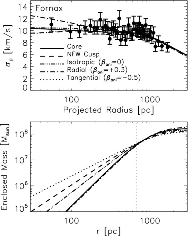
(Credit: Walker & Peñarrubia 2011)
Even though there is lots of data on the velocity dispersion at different radii, the data is consistent with either a cored or a cuspy profile and the difference between cored and cuspy is similar to the range spanned by models with different values of \(\beta\). The bottom panel of the figure above again shows that all of the different mass and \(\beta\) models agree on the enclosed mass at a radius that is close to the half-mass radius.
Spectroscopic studies of dSphs around the Milky Way have shown that these galaxies consist of multiple sub-populations with different chemical abundances and density profiles. For example, Tolstoy et al. (2004) found two populations in the Sculptor galaxy, with a centrally-concentrated metal-rich population, and a more diffuse metal-poor population. Similar studies of other dSphs have shown similar results. This presumably happens because these populations form at different times in the life of the dSph, when star-formation is happening on different spatial scales. Because these sub-populations have different spatial distributions, they have different \(R_e\) and \(r_{1/2}\) and will therefore measure the enclosed mass at different radii (see Equation \(\ref{eq-wolf-rhalf}\)). Therefore, conceptually we can proceed as follows: obtain spectroscopic data for many stars in dSphs, split them into distinct chemical populations using their chemical abundances, and obtain the enclosed mass \(M(<r_{1/2,i})\) at the different \(\{r_{1/2,i}\}\) of these populations. The profile \([r_{1/2,i},M(<r_{1/2,i})]\) is then a robust measurement of the mass profile and we can, for example, determine the slope \(\Gamma = \mathrm{d} \ln M / \mathrm{d} \ln r\).
An analysis of this sort was performed by Walker & Peñarrubia (2011) for the Carina, Sculptor, and Fornax dSphs, although the details of the implementation are slightly more complicated than what we have presented here. For Carina they did not find evidence for two distinct sub-populations and they could therefore only determine the mass at a single radius. But for Sculptor and Fornax they were able to probabilistically split the data into two populations, determine \(M(<r)\) at two different radii, and constrain \(\Gamma\). Their results are displayed in the following figure:
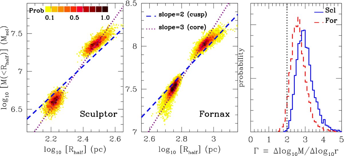
(Credit: Walker & Peñarrubia 2011)
From the definition of \(\Gamma\), it is clear that a cored profile with \(\rho(r) \propto \mathrm{constant}\) would give \(M(<r) \propto r^3\) and therefore \(\Gamma = 3\), while a cuspy profile \(\rho(r) \propto 1/r\) would give \(M(<r) \propto r^2\) and \(\Gamma = 2\). The data are inconsistent with a cuspy profile at the 95% (for Sculptor) to 99.8% confidence level (for Fornax).
Using simple equilibrium dynamical modeling applied to two tracer sub-populations, we can therefore robustly determine the inner dark-matter slopes of dSphs and rule out that these have the cuspy profile expected from cosmological simulations of the formation of dark matter halos. Instead, these dark-matter halos appear to have constant-density cores with sizes of a few hundred parcsecs. This could be because the popular cold-dark-matter model is incorrect or it could result from gravitational interactions between the few stars that these dwarf galaxies contain and the dark matter in their centers. In particular, enough of the energy released in explosions of massive stars as supernovae might be transfered as gravitational energy to the dark matter distribution (this is a type of baryonic feedback). For such gravitational-energy injection to significantly change the phase-space density of dark matter, it has to happen non-adiabatically, that is, on time scales that are short with respect to the dynamical time.
We can explore how non-adiabatic energy injection can destroy a central dark-matter cusp and turn it into a core using the tools from Chapter 6. In particular, we can model the dark-matter distribution in a dSphs with an isotropic Hernquist distribution, for which we determined the equilibrium distribution function in Chapter 6.6.1. Let’s use Fornax as an example. We model Fornax as an isotropic Hernquist profile with a total mass \(M = 3\times 10^8\,M_\odot\) and a scale radius \(a = 1\,\mathrm{kpc}\). We then sample this profile with \(10^6\) particles:
[230]:
from galpy.potential import HernquistPotential
from galpy.df import isotropicHernquistdf
totmass= 3.*1e8*u.Msun
hp= HernquistPotential(amp=2.*totmass,a=1.*u.kpc)
dfh= isotropicHernquistdf(pot=hp)
samp= dfh.sample(n=int(1e6))
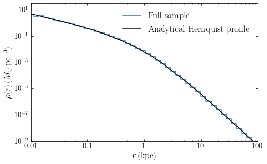
We can determine the density profile of the samples and compare it to the analytical profile, which shows excellent agreement:
[233]:
from matplotlib.ticker import FuncFormatter
bins= 101
def plot_sample_density(samp,bins,weights,rrange=None,r_plot_unit=u.pc,
                       label=None):
    w,e= numpy.histogram(numpy.log(samp.r().to_value(u.pc)),
                         bins=bins,range=rrange,weights=weights)
    binrs= numpy.exp((numpy.roll(e,-1)+e)[:-1]/2.)
    ploty= w/(4.*numpy.pi*binrs**3.*(e[1]-e[0]))
    loglog(binrs*(u.pc/r_plot_unit).to(u.dimensionless_unscaled),
           ploty,drawstyle='steps-mid',label=label)
    return binrs*u.pc
plotrs= plot_sample_density(samp,bins,totmass*numpy.ones(samp.size)/samp.size,
                            r_plot_unit=u.kpc,
                           label=r'$\mathrm{Full\ sample}$')
plot(plotrs.to(u.kpc),hp.dens(plotrs,0.),color='k',
    label=r'$\mathrm{Analytical\ Hernquist\ profile}$')
xlabel(r'$r\,(\mathrm{kpc})$')
ylabel(r'$\rho(r)\,(M_\odot\,\mathrm{pc}^{-3})$')
xlim(0.01,100)
ylim(1e-9,3e1)
gca().xaxis.set_major_formatter(FuncFormatter(
                lambda y,pos: (r'${{:.{:1d}f}}$'.format(int(\
                    numpy.maximum(-numpy.log10(y),0)))).format(y)))
legend(frameon=False,fontsize=18.);
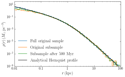
Next we want to inject gravitational energy in this sample in a non-adiabatic way. We will do this by perturbing all of the velocities with perturbation velocities drawn from an isotropic Gaussian distribution characterized by a dispersion \(\sigma\). This mimics non-adiabatic heating. This instantaneous heating places the system out of equilibrium, so we integrate all orbits for 500 Myr to see what new equilibrium state the system settles in. Integrating all \(10^6\) particles would take a long time, so we only consider a subsample. Because we want to focus on what will happen in the inner regions, we sample approximately equal numbers in equal logarithmic bins in radius. The following code does this subsampling and orbit integration, and it computes the weights of each subsampled particle such that they faithfully represent the underlying phase-space density:
[243]:
# Assumes that n << samp.size
def logr_sample(samp,n):
    return samp[numpy.random.choice(numpy.arange(samp.size),size=n,replace=False,
                                    p=1./samp.r()/numpy.sum(1./samp.r()))]
subsamp= logr_sample(samp,30000)
subsamp_weight= subsamp.r()/(numpy.sum(subsamp.r()))\
        *totmass.to_value(u.Msun)
ts= numpy.linspace(0.,0.5,101)*u.Gyr
subsamp.integrate(ts,hp,method='dop853_c')
We can compare the density profile of the original sample to that of the subsample at \(t=0\) and after 500 Myr. All agree well with the analytical profile, to within the sampling noise:
[234]:
plotrs= plot_sample_density(samp,bins,
                            totmass*numpy.ones(samp.size)/samp.size,
                            r_plot_unit=u.kpc,
                            label=r'$\mathrm{Full\ original\ sample}$')
plot_sample_density(subsamp,bins,subsamp_weight,r_plot_unit=u.kpc,
                    label=r'$\mathrm{Original\ subsample}$')
plot_sample_density(subsamp(ts[-1]),bins,subsamp_weight,r_plot_unit=u.kpc,
                    label=r'$\mathrm{Subsample\ after\ 500\ Myr}$')
plot(plotrs.to(u.kpc),hp.dens(plotrs,0.),color='k',
    label=r'$\mathrm{Analytical\ Hernquist\ profile}$')
xlabel(r'$r\,(\mathrm{kpc})$')
ylabel(r'$\rho(r)\,(M_\odot\,\mathrm{pc}^{-3})$')
xlim(0.01,100)
ylim(1e-9,3e1)
gca().xaxis.set_major_formatter(FuncFormatter(
                lambda y,pos: (r'${{:.{:1d}f}}$'.format(int(\
                    numpy.maximum(-numpy.log10(y),0)))).format(y)))
legend(frameon=False,fontsize=18.);
Next we heat the particles in the subsample, by adding velocities drawn from an isotropic Gaussian. To mimic that this heating only happens in the inner part of the galaxy where stars are abundant, we only heat stars within 1 kpc:
[225]:
from galpy.orbit import Orbit
from galpy.util import coords
def heat_orbits(samp,sigma,rmax):
    new_vx= samp.vx()+numpy.random.normal(size=samp.size)*sigma*(samp.r() < rmax)
    new_vy= samp.vy()+numpy.random.normal(size=samp.size)*sigma*(samp.r() < rmax)
    new_vz= samp.vz()+numpy.random.normal(size=samp.size)*sigma*(samp.r() < rmax)
    new_vR, new_vT, _= coords.rect_to_cyl_vec(new_vx,new_vy,new_vz,
                                              samp.R(),samp.phi(),samp.z(),
                                              cyl=True)
    return Orbit([samp.R(),new_vR,new_vT,samp.z(),new_vz,samp.phi()])
def heat_subsample(samp,sigma,rmax):
    heated_subsamp= heat_orbits(subsamp,sigma,rmax=1.*u.kpc)
    ts= numpy.linspace(0.,.5,101)*u.Gyr
    heated_subsamp.integrate(ts,hp)
    return heated_subsamp
We can then compare the resulting density distribution for different levels of heating (note that the velocity dispersion of the dark matter is \(\approx 10\,\mathrm{km\,s}^{-1}\) for the unperturbed system):
[244]:
plotrs= plot_sample_density(subsamp(ts[-1]),bins,subsamp_weight,
                            r_plot_unit=u.kpc,
                            label=r'$\mathrm{Heating}\ \sigma = 0$')
heated_subsamp= heat_subsample(subsamp,10.*u.km/u.s,rmax=1.*u.kpc)
plotrs= plot_sample_density(heated_subsamp(ts[-1]),bins,subsamp_weight,
                            r_plot_unit=u.kpc,
                            label=r'$\mathrm{Heating}\ \sigma = 10\,\mathrm{km\,s}^{-1}$')
heated_subsamp= heat_subsample(subsamp,20.*u.km/u.s,rmax=1.*u.kpc)
plotrs= plot_sample_density(heated_subsamp(ts[-1]),bins,subsamp_weight,
                            r_plot_unit=u.kpc,
                            label=r'$\mathrm{Heating}\ \sigma = 20\,\mathrm{km\,s}^{-1}$')
heated_subsamp= heat_subsample(subsamp,40.*u.km/u.s,rmax=1.*u.kpc)
plotrs= plot_sample_density(heated_subsamp(ts[-1]),bins,subsamp_weight,
                            r_plot_unit=u.kpc,
                            label=r'$\mathrm{Heating}\ \sigma = 40\,\mathrm{km\,s}^{-1}$')
plot(plotrs.to(u.kpc),hp.dens(plotrs,0.),color='k',
    label=r'$\mathrm{Analytical\ Hernquist\ profile}$')
xlabel(r'$r\,(\mathrm{kpc})$')
ylabel(r'$\rho(r)\,(M_\odot\,\mathrm{pc}^{-3})$')
xlim(0.01,100)
ylim(1e-9,3e1)
gca().xaxis.set_major_formatter(FuncFormatter(
                lambda y,pos: (r'${{:.{:1d}f}}$'.format(int(\
                    numpy.maximum(-numpy.log10(y),0)))).format(y)))
legend(frameon=False,fontsize=18.);
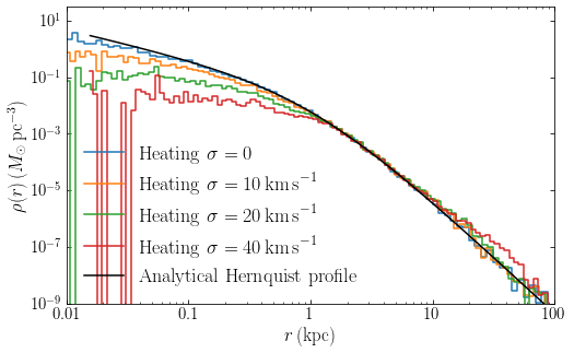
We see that the heating indeed causes a core to form (the density in the center becomes constant with radius) and that the size of the core depends on the amount of heating applied, with larger values corresponding to larger cores. Thus, to create a core with a size of a few hundred pc, we need to heat the dark-matter distribution by \(\approx 20\,\mathrm{km\,s}^{-1}\).
The standard explanation for the source of this heating (e.g., Pontzen & Governato 2012) is that it comes from the non-adiabatic changes in the stellar-mass profile that result from repeated supernova explosions of massive stars. Thus, eventually, the source of this gravitational energy has to be related to the energy released by supernovae of massive stars. The total amount of gravitational energy required is \(\approx M(r<1\,\mathrm{kpc})\,\sigma^2 /2 \approx 3\times 10^{53}\,\mathrm{erg}\) (this estimate agrees well with more sophisticated treatments, e.g., Peñarrubia et al. 2012). We can compare that number to the total amount of energy released by supernovae in Fornax, which has a stellar mass of \(\approx 3\times 10^7\,M_\odot\), corresponding to about \(10^8\) stars. According to the standard Kroupa (2001) initial mass function \(\mathrm{d} N / \mathrm{d} M\) of stars, 0.37% of stars have high enough mass (\(M > 8\,M_\odot\)) to explode as a supernova, or about \(3.7\times 10^5\) for the total stellar population of Fornax. Each supernova releases about \(10^{51}\,\mathrm{erg}\), or a total of \(3.7\times 10^{56}\,\mathrm{erg}\) for Fornax’s stars. Thus, there is plenty of energy released in supernovae available for heating the dark-matter gravitational potential and even transferring only a fraction of 1% of the energy released in supernovae to the dark-matter distribution is enough to turn the cusps predicted by the standard cold-dark-matter paradigm into the observed cores.