
15. Equilibria of elliptical galaxies and dark matter halos
Just like for spherical systems (discussed in Chapter 6) and disk galaxies (Chapter 11), steady-state configurations of elliptical galaxies and (non-spherical) dark-matter halos are of high interest. Indeed, in many ways understanding equilibrium states and performing equilibrium dynamical modeling is more important for elliptical galaxies than it is for disks, because we can learn much about the dynamical structure and mass distribution of disk galaxies (including the existence of dark matter as discussed in Chapter 9!) from the kinematics of closed, circular gas orbits. Gas or any sort of disk component is rare or subdominant in elliptical galaxies (e.g., Rix & White 1990), so we cannot simply observe tracers on circular orbits and directly constrain the mass profile using the relation between circular velocity and enclosed mass. Modeling spheroidally or ellipsoidally distributed tracers with equilibrium modeling is therefore one of the only ways to constrain the orbital structure, mass profiles, and dark matter content of elliptical galaxies (the other main method being gravitational lensing)
But equilibrium modeling of elliptical galaxies is significantly more complicated than in the case of spherical mass distributions or disks, where the existence of multiple integrals of motion (especially in the spherical case where there are four) and the ordered, close-to-circular nature of orbits (for disks) makes it possible to analyze realistic systems with analytical tools. While similar analytical results can be obtained for spheroidal or even triaxial systems—for example, one can work out the Jeans equations in spheroidal or ellipsoidal coordinates, or write down distribution functions for oblate and prolate models, or triaxial models of Staeckel form—these results are far less useful, because they require so many assumptions as to not be applicable to realistic galaxies. (However, they can be very useful for testing the more general, numerical tools used to model elliptical galaxies).
In this chapter, we discuss two main topics useful in the study of spheroidal or ellipsoidal systems: a generalization of the virial theorem first derived in Chapter 6.2 to tensor form, the tensor-virial theorem, that provides a relation between the integrated radial profile, shape, and 3D kinematics that allows us to understand how the shape of elliptical galaxies is sustained by their internal kinematics. Then we will discuss the main numerical technique used to investigate possible equilibrium configurations of complex elliptical galaxies and dark-matter halos and to perform dynamical modeling of observations of the surface density and kinematics of elliptical galaxies, Schwarzschild modeling. Examples of the dynamical modeling techniques discussed in this chapter to observations of elliptical galaxies are discussed further in Chapter 17.
15.1. The tensor virial theorem
We introduced the virial theorem in Chapter 6.2 and specified there that the theorem that we derived was more specifically known as the scalar virial theorem. The scalar virial theorem is a simple, yet powerful tool for understanding the overall structure and mass distribution of a gravitating system. For example, using it to estimate the mass of a gravitating system (like we did in Chapter 6.2 with globular clusters to determine the Milky Way’s mass) allowed Fritz Zwicky to uncover the first evidence for dark matter from the large velocity dispersion of galaxies in the Coma cluster. Or later in Chapter 18.2.2, we will use the virial theorem to determine the size of a just-formed, virialized dark-matter halo. But while the scalar virial theorem can give us much information about the overall mass of a system, it is a blunt tool to understand more complex systems such as elliptical galaxies and other flattened systems.
15.1.1. Collisional systems
We can derive a more sophisticated, tensorial form of the virial theorem by starting from the virial tensor \(\vec{G}_{\alpha\beta}\) rather than the scalar virial that we used in Chapter 6.2
where \(x^\alpha_i\) is the \(\alpha\)-th component of the position vector \(\vec{x}\) of particle \(i\), \(v^\beta_i\) is the \(\beta\)-th component of the velocity vector \(\vec{v}_i\) of particle \(i\), and the \(w_i\) are an arbitrary set of weights. Note that we have explicitly defined the tensor so as to be symmetric. By comparing to the definition of the scalar virial \(G\) in Equation (6.14), we see that \(G\) is simply the trace of \(\vec{G}_{\alpha\beta}\). Again assuming that the system of \(N\) particles is in equilibrium, we can set \(\mathrm{d} \vec{G}_{\alpha\beta} / \mathrm{d}t = 0\), which gives
where \(g^\beta(\vec{x})\) is the \(\beta\)-th component of the gravitational field at \(\vec{x}\).
The gravitational field \(\vec{g}(\vec{x})\) can either be an external field, in which case it can simply be plugged into the expression above, or it can be the field resulting from the mutual gravity between all of the \(N\) objects in the system. In the latter case, we can re-write the last two terms of Equation (\ref{eq-tensorvirial-first}) with a similar set of manipulations as in Equations (6.19); we define this tensor to be twice the potential-energy tensor \(\vec{W}_{\alpha\beta}\) of a system of point particles
where \((\alpha \leftrightarrow \beta)\) indicates that we repeat the first term with the \(\alpha\) and \(\beta\) indices swapped. When we set \(w_i \equiv m_i\) for all particles, this simplifies to
or using the symmetry under \(i\leftrightarrow j\)
Similarly, we define the kinetic energy tensor \(\vec{K}_{\alpha\beta}\) as
and then Equation (\ref{eq-tensorvirial-first}) can be written as
This is the tensor virial theorem. In a steady state system, \(\mathrm{d} \vec{G}_{\alpha\beta} / \mathrm{d}t = 0\), such that this becomes
Taking the trace of this equation, we obtain the scalar virial theorem of Equation (6.23) again.
15.1.2. Collisionless systems
For collisionless systems, such as dark-matter halos or smooth models of galaxies, we can derive a continuous version of the tensor (and scalar) virial theorem. To do this, we define the virial tensor with weights \(w(\vec{x}) = \rho(\vec{x},t)\,\mathrm{d} \vec{x}\), using the mean velocity \(\bar{\vec{v}}(\vec{x},t)\) for the velocity, and we integrate over all of position space
Because \(\bar{\vec{v}}(\vec{x},t) = \int\mathrm{d}\vec{v}\,f(\vec{x},\vec{v},t)/\rho(\vec{x},t)\), where \(f(\vec{x},\vec{v},t)\) is the distribution function, we can also write this as
which is indeed a natural definition of the virial tensor for a collisionless system (for which the phase-space distribution function is the fundamental quantity). Again taking the time derivative, we obtain now
where we have used the fact that the total time derivative of the distribution function vanishes (Liouville’s theorem; Equation [6.37]). We again split the right-hand side of this equation into a kinetic- and potential-energy tensor. First, we define the kinetic energy tensor for continuous, collisionless systems as
We can also write this as
where \(\vec{T}_{\alpha\beta}\) and \(\vec{\Pi}_{\alpha\beta}\) are the contributions from ordered and random motion to the kinetic energy
where \(\vec{\sigma}_{\alpha\beta}\) is the velocity dispersion tensor.
The last two terms of Equation \(\eqref{eq-tensorvirial-cont-first}\) are the potential energy tensor and can be worked out as
which is symmetric under \(\alpha \leftrightarrow\beta\) and thus the potential energy tensor for a continuous system simplifies to
With these expressions for the components of the kinetic energy tensor and the potential energy tensor, we can write the tensor virial theorem for a collisionless system as
For an equilibrium, collisionless system, we obtain
Taking the trace, we obtain the scalar virial theorem for a continuous, collisionless system
where the kinetic terms are
and they combine to the scalar kinetic energy
where \(v = |\vec{v}|\) and the \(\langle \cdot \rangle\) averaging is over all dimensions of phase space (rather than just the velocity averaging of \(\bar{\cdot}\)).
The scalar potential energy of the system is
By using the Poisson equation, we can obtain an alternative form as (dropping the [\(\vec{x},t\)] arguments to reduce clutter)
where we used integration-by-parts to re-write the second term. After another round of integration by parts we get
and because in three dimensions, there are twice as many \(j \neq i\) as there are \(j = i\), this can be simplified to
such that after applying the Poisson equation again, we find the following simple expression:
By considering the amount of work necessary to move a small amount of mass from infinity to position \(\vec{x}\), it can be shown that this scalar potential energy is the total work necessary to assemble the mass distribution \(\rho(\vec{x}\)).
15.1.3. Properties and examples of the potential energy tensor
Because we will be using the potential energy tensor and its scalar form later in this chapter and also in later chapters, it is worth discussing it in a little more detail. In this section, we discuss some general properties of the potential energy tensor and we calculate it for a few example cases that we will use later.
For a spherical mass distribution, the potential energy tensor is particularly simple. The general expression from Equation \(\eqref{eq-pot-energy-tensor}\) for a spherical mass distribution becomes
From the definition of spherical coordinates in Equations (A.1–A.3), it is straightforward to compute that the inner integral \(\int \mathrm{d}\theta\,\mathrm{d}\phi\,\sin\theta\,x^\alpha\,x^\beta = -4\pi\,r^2\delta^{\alpha\beta}/3\), where \(\delta^{\alpha\beta}\) is the Kronecker delta, and therefore
or using the relation between the radial component of the gravitational field and the enclosed mass (Equation [3.29])
Thus, the potential energy tensor for a spherical mass distribution is diagonal and furthermore, because the expression does not depend on the \(\alpha\) and \(\beta\) indices except for the Kronecker delta, it is isotropic with all elements on the diagonal equal. The scalar potential energy is therefore
An example that we will use in Chapter 18 is the potential energy of a homogeneous sphere (see Chapter 3.4.2). Because the enclosed mass for the homogeneous sphere is \(M(<r) = 4\pi\,\rho_0\,r^3/3\) and the density is zero at \(r \geq R\), we have
where \(M = 4\pi\,\rho_0\,R^3/3\) is the total mass.
Another example is that of a thin spherical shell, which is useful to compare to the thin oblate shell that we will discuss below. For a thin shell of mass \(M\) at radius \(R\), which we first encountered in Chapter 3.2, we have that \(\rho(r) = M\delta(r-R)/[4\pi\,R^2]\) and \(\partial \Phi/\partial r = GM\,\Theta(r-R)/r^2\) where \(\Theta(r)\) is the Heaviside function. Thus, Equation \eqref{eq-potenergytensor-sphere} gives
because \(\int\mathrm{d}r\,r\,\delta(r-R)\,\Theta(r-R) = R/2\) (see Equation B.10).
For an axisymmetric mass distribution symmetric with respect to rotation around \(z\), the potential energy tensor similarly simplifies. The general expression from Equation \(\eqref{eq-pot-energy-tensor}\) now becomes
Thus, for an axisymmetric mass distribution, the potential energy tensor is diagonal as well and \(W_{xx} = W_{yy}\).
To better understand the potential energy tensor for non-spherical systems, we can write \(\vec{W}_{\alpha\beta}\) in a form similar to that in Equation \eqref{eq-potenergytensor-collisional} (for simplicity, we drop the time dependence in the following equations)
which is the continuous limit of Equation \eqref{eq-potenergytensor-collisional} and can be derived from Equation \eqref{eq-pot-energy-tensor} by using that \(\Phi(\vec{x}) = \int \mathrm{d}\vec{x}'\,\rho(\vec{x}')/|\vec{x}'-\vec{x}|\). Because the numerator of the final factor is the only place that the indices \(\alpha\) and \(\beta\) appear, this expression makes it clear that the relative magnitude of the diagonal elements is set by the distribution of \(|x'^\alpha-x^\alpha|\) of the mass distribution. For a system that is flattened along the \(z\) axis, the typical magnitude of \(|z'-z|\) is less than that of \(|x'-x'|\) and \(|y'-y|\) and therefore \(W_{zz}/W_{xx} < 1\) and \(W_{zz}/W_{yy} < 1\). For an oblate, axisymmetric system, \(W_{zz}/W_{xx} = W_{zz}/W_{yy} < 1\).
To understand the dynamical structure of elliptical galaxies, it is useful to approximate them as oblate spheroids (see Chapter 13.2), where the density is only a function of the coordinate \(m\) defined as
with \(q \leq 1\). As discussed in Chapter 13.2, this means that the density in \((R,z)\) is constant on the ellipses with eccentricity \(e = \sqrt{1-q^2}\). Because this model is axisymmetric, the potential-energy tensor is diagonal and its diagonal components can be calculated using Equation \eqref{eq-potenergy-axi} above. This gives
where \(M\) is the mass of the shell, \(m_0\) is its spheroidal radius, and \(A_i(q)\) are functions that are typically expressed as a function of the eccentricity \(e = \sqrt{1-q^2}\) of the shell and which are given by
Because \(A_x(0) = A_z(0) = 2/3\), it is clear that in the limit of a spherical shell, Equations \eqref{eq-potenergytensor-oblateshell-1} and \eqref{eq-potenergytensor-oblateshell-2} reduce to the corresponding expression of Equation \eqref{eq-potenergytensor-sphericalshell} for a spherical shell.
The ratio of the \(zz\) and \(xx\) components of the potential-energy tensor for a thin oblate spheroidal shell is then given by (we express all occurrences of the axis ratio \(q\) in terms of the eccentricity)
The functional behavior of this ratio for eccentricities between 0 (spherical) and 1 (razor-thin) is as follows
[4]:
def Wzz_over_Wxx(e):
    return 2.*(1.-e**2.)*(1./numpy.sqrt(1.-e**2.)-numpy.arcsin(e)/e)/(numpy.arcsin(e)/e-numpy.sqrt(1.-e**2.))
# To better resolve the behavior near e=1, use a denser grid there
e_WzzWxx= numpy.hstack((numpy.linspace(1e-4,0.5,51),
                     sorted(1.-numpy.geomspace(1e-4,0.5,51))))
plot(e_WzzWxx,Wzz_over_Wxx(e_WzzWxx))
xlabel(r'$e$')
ylabel(r'$W_{zz}/W_{xx}$')
ylim(0.0,1.05);
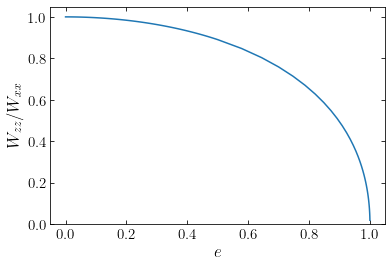
As expected, the ratio is equal to one for a spherical shell and smaller than one for flattened shells.
Equation \eqref{eq-Wzz-over-Wxx-oblateshell} furthermore demonstrates that the ratio \(W_{zz}/W_{xx}\) is only a function of the axis ratio of the oblate shell, not of its radius or mass. Another way of stating this is to say that the ratio \(W_{zz}/W_{xx}\) depends only on the shape of the oblate shell, but not on its radial structure. Remarkably, this result continues to hold for an extended density distribution that is constant on similar spheroids, as was shown by Roberts (1962) (indeed, Roberts 1962 actually showed that this holds for any extended density distribution that is constant on similar ellipsoids). Thus, the ratio \(W_{zz}/W_{xx}\) of any oblate density distribution that is constant on similar spheroids is given by Equation \eqref{eq-Wzz-over-Wxx-oblateshell}.
We can test that this is the case by computing the potential energy tensor for different, non-trivial oblate density distributions. First, we implement the calculation of the potential-energy tensor for an axisymmetric distribution using Equation \eqref{eq-potenergy-axi}
[4]:
from scipy import integrate
from galpy.potential import evaluateRforces, evaluatezforces, evaluateDensities
def potenergy_tensor_axi(pot,component='xx',Rmin=0.,Rmax=numpy.inf,zmin=lambda R: 0., zmax= lambda R: numpy.inf):
    if component[0] != component[1]:
        return 0.
    if component == 'xx' or component == 'yy':
        def integrand(z,R):
            return evaluateDensities(pot,R,z,phi=0.)*R**2.*evaluateRforces(pot,R,z,phi=0.)
    elif component == 'zz':
        def integrand(z,R):
            return 2.*evaluateDensities(pot,R,z,phi=0.)*R*z*evaluatezforces(pot,R,z,phi=0.)
    else:
        return RuntimeError('Component {} not understood'.format(component))
    return 2.*numpy.pi*integrate.dblquad(integrand,Rmin,Rmax,zmin,zmax)[0]
While for density distributions without sharp edges, we will generally integrate over all of space, we have allowed the option to specify the integration range so we can test this function against the expression for the potential-energy tensor of the homogeneous sphere in Equation \eqref{eq-potenergytensor-homogsphere}.
[75]:
from galpy.potential import HomogeneousSpherePotential
Rmax= 3.
hp= HomogeneousSpherePotential(amp=2.,R=Rmax)
print('Wxx = {:.3f}, Wzz = {:.3f}, analytic Wxx = Wzz = {:.3f}'.format(
    potenergy_tensor_axi(hp,component='xx',Rmax=Rmax,zmax=lambda R: numpy.sqrt(Rmax**2.-R**2.)),
    potenergy_tensor_axi(hp,component='zz',Rmax=Rmax,zmax=lambda R: numpy.sqrt(Rmax**2.-R**2.)),
    -3./5.*hp.mass(Rmax)**2./Rmax/3.))
Wxx = -777.600, Wzz = -777.600, analytic Wxx = Wzz = -777.600
Thus, we see that we get the correct result for the homogeneous sphere.
Next, we compute the \(W_{xx}\) and the ratio \(W_{zz}/W_{xx}\) for flattened Hernquist distributions (for which the density \(\rho(m)\) is that of the Hernquist sphere of Chapter 3.4.6). First, we define some utility functions to go back and forth between \(q\) and \(e\)
[5]:
def q_from_e(e):
    return numpy.sqrt(1.-e**2.)
def e_from_q(q):
    return numpy.sqrt(1.-q**2.)
and then we compute the tensor for \(e = 0.1\) to \(e=0.9\) in \(\delta e = 0.1\) increments. We can then compare these values to what Equation \eqref{eq-Wzz-over-Wxx-oblateshell} predicts:
[92]:
from galpy.potential import TriaxialHernquistPotential
es_hernq_a3= numpy.arange(0.1,1.0,0.1)
a= 3.
Wxx_hernq_a3= numpy.zeros_like(es_hernq_a3)
Wzz_hernq_a3= numpy.zeros_like(es_hernq_a3)
for ii,e in enumerate(es_hernq_a3):
    thp= TriaxialHernquistPotential(a=a,c=q_from_e(e))
    Wxx_hernq_a3[ii]= potenergy_tensor_axi(thp,component='xx')
    Wzz_hernq_a3[ii]= potenergy_tensor_axi(thp,component='zz')
plot(e_WzzWxx,Wzz_over_Wxx(e_WzzWxx))
plot(es_hernq_a3,Wzz_hernq_a3/Wxx_hernq_a3,'o')
xlabel(r'$e$')
ylabel(r'$W_{zz}/W_{xx}$')
ylim(0.0,1.05);
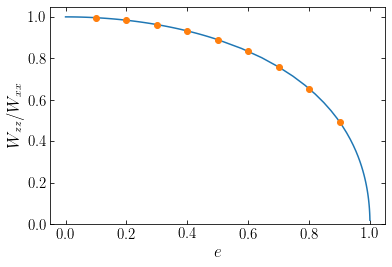
We see that they agree very well! Let’s change the radial density structure by choosing a different scale parameter \(a\) and show both these new models and the previous ones (choosing a different grid in \(e\) so they do not fully overlap):
[87]:
es_hernq_a6= numpy.arange(0.05,1.05,0.1)
a= 6.
Wxx_hernq_a6= numpy.zeros_like(es_hernq_a6)
Wzz_hernq_a6= numpy.zeros_like(es_hernq_a6)
for ii,e in enumerate(es_hernq_a6):
    thp= TriaxialHernquistPotential(a=a,c=q_from_e(e))
    Wxx_hernq_a6[ii]= potenergy_tensor_axi(thp,component='xx')
    Wzz_hernq_a6[ii]= potenergy_tensor_axi(thp,component='zz')
plot(e_WzzWxx,Wzz_over_Wxx(e_WzzWxx))
plot(es_hernq_a3,Wzz_hernq_a3/Wxx_hernq_a3,'o')
plot(es_hernq_a6,Wzz_hernq_a6/Wxx_hernq_a6,'d')
xlabel(r'$e$')
ylabel(r'$W_{zz}/W_{xx}$')
ylim(0.0,1.05);
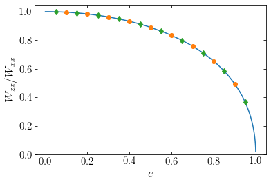
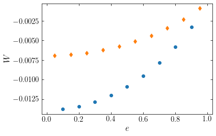
All of the points for the different models agree with the analytic prediction. Showing instead the scalar potential energy (the trace of the tensor, \(W = 2W_{xx}+W_{zz}\) in the axisymmetric case) as a function of \(e\) for the different models, we see that they are different
[90]:
plot(es_hernq_a3,2.*Wxx_hernq_a3+Wzz_hernq_a3,'o')
plot(es_hernq_a6,2.*Wxx_hernq_a6+Wzz_hernq_a6,'d')
xlabel(r'$e$')
ylabel(r'$W$')
xlim(-0.03,1.03);
To completely change the radial structure, we can also consider a completely different density profile, that of the perfect ellipsoid
[91]:
from galpy.potential import PerfectEllipsoidPotential
es_pellips_a4= numpy.arange(0.075,1.075,0.1)
a= 4.
Wxx_pellips_a4= numpy.zeros_like(es_pellips_a4)
Wzz_pellips_a4= numpy.zeros_like(es_pellips_a4)
for ii,e in enumerate(es_pellips_a4):
    thp= PerfectEllipsoidPotential(a=a,c=q_from_e(e))
    Wxx_pellips_a4[ii]= potenergy_tensor_axi(thp,component='xx')
    Wzz_pellips_a4[ii]= potenergy_tensor_axi(thp,component='zz')
plot(e_WzzWxx,Wzz_over_Wxx(e_WzzWxx))
plot(es_hernq_a3,Wzz_hernq_a3/Wxx_hernq_a3,'o')
plot(es_hernq_a6,Wzz_hernq_a6/Wxx_hernq_a6,'d')
plot(es_pellips_a4,Wzz_pellips_a4/Wxx_pellips_a4,'d')
xlabel(r'$e$')
ylabel(r'$W_{zz}/W_{xx}$')
ylim(0.0,1.05);
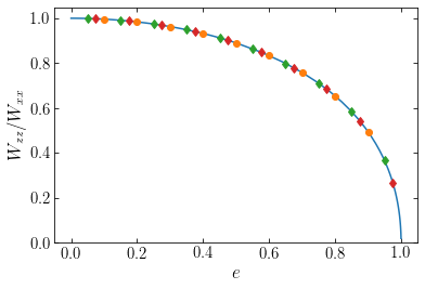
We again find good agreement, further demonstrating that the ratio \(W_{zz}/W_{xx}\) is independent of the radial structure of the oblate mass model and only depends on the distribution’s shape, that is, its axis ratio. In the next section we will exploit this property to better understand the dynamical structure of elliptical galaxies.
15.2. Are elliptical galaxies flattened by rotation?
Now that we have derived the tensor-virial theorem and now that we understand the potential-energy tensor of oblate spheroids, we can use the tensor-virial theorem to understand the basic dynamical structure of elliptical galaxies. We will focus here on axisymmetric elliptical galaxies and ask the question “Is the oblateness of such elliptical galaxies caused by rotation?”. What we mean more specifically with this question is the following. Observations of elliptical galaxies demonstrate that the velocity dispersion of stars is much larger than that of stars in disk galaxies. Unlike for disk galaxies, the dynamical support against gravitational collapse for elliptical galaxies therefore comes from their velocity dispersion rather than ordered rotation and we say that elliptical galaxies are pressure-supported systems. However, a non-rotating system with an isotropic velocity-dispersion tensor has to be spherical, as is clear from the tensor virial theorem with \(\vec{T}_{\alpha\beta} = 0\) (for zero rotation):
If \(\vec{\Pi}_{\alpha\beta} = M\,\sigma^2\,\delta^{\alpha\beta}\) then \(\vec{W}_{\alpha\beta} \propto \delta^{\alpha\beta}\) as well and this is only the case for a spherical system (see the argument following Equation \ref{eq-pot-energy-tensor-likecollisional}). There are, therefore, two ways in which a gravitational system can be flattened: (i) through rotation, such that \(\vec{T}_{\alpha\beta} \neq 0 \neq \delta^{\alpha\beta}\), or (ii) through an anisotropic velocity dispersion tensor. The question “Are elliptical galaxies flattened by rotation?” therefore specifically asks whether elliptical galaxies can be rotation alone, that is, by having the galaxy rotate while keeping the velocity dispersion isotropic.
Let’s therefore consider a model for an elliptical galaxy that is a flattened spheroid with an axis ratio \(q\) and that has an overall rotation around the \(z\) axis with a velocity \(v\) and isotropic velocity dispersion \(\sigma\). For this model,
that is, only the \(xx\) and \(yy\) diagonal elements are non-zero and the total kinetic energy in rotation is \(T_{xx}+T_{yy}=Mv^2/2\). We also have
The tensor-virial theorem then states that
If we then take the ratio of the \(xx\) and \(zz\) components of this equation, we obtain
or
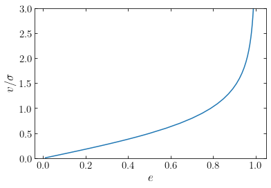
This equation makes sense in that for a spherical system, \(W_{xx}/W_{zz} = 1\), so \(v/\sigma = 0\) corresponding to the fact that a spherical, isotropic system does not rotate. For a flattened system, \(W_{xx}/W_{zz} > 1\), so \(v/\sigma > 0\).
For an oblate spheroid, we know that the ratio \(W_{xx}/W_{zz}\) only depends on the axis ratio \(q\) (Equation \ref{eq-Wzz-over-Wxx-oblateshell}), so we have that
where \(F(q) = W_{xx}/W_{zz}\) is the inverse of Equation \eqref{eq-Wzz-over-Wxx-oblateshell}, or explicitly (using the eccentricity \(e = \sqrt{1-q^2}\) instead of \(q\))
Let’s see what this function looks like
[6]:
# To better resolve the behavior near e=1, use a denser grid there
e_vsigma= numpy.hstack((numpy.linspace(1e-4,0.5,51),
                     sorted(1.-numpy.geomspace(1e-4,0.5,51))))
#Wzz_over_Wxx(.) defined in the previous section
plot(e_vsigma,numpy.sqrt(2./Wzz_over_Wxx(e_vsigma)-2.))
xlabel(r'$e$')
ylabel(r'$v/\sigma$')
ylim(0.,3.);
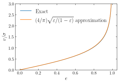
Remarkably, to an accuracy of about one percent over the entire range of axis ratios, this function can also be approximated as (Kormendy 1982)
or in terms of the ellipticity \(\varepsilon = 1-q\) (not to be confused with the eccentricity)
Comparing this approximation to the full expression from Equation \eqref{eq-tensorvirial-vsigmaellip-full}, we see that they agree very well:
[27]:
# To better resolve the behavior near e=1, use a denser grid there
e_vsigma= numpy.hstack((numpy.linspace(1e-4,0.5,51),
                     sorted(1.-numpy.geomspace(1e-4,0.5,51))))
#Wzz_over_Wxx(.) defined in the previous section
plot(e_vsigma,numpy.sqrt(2./Wzz_over_Wxx(e_vsigma)-2.),
     label=r'$\mathrm{Exact}$')
plot(e_vsigma,4./numpy.pi*numpy.sqrt((1-q_from_e(e_vsigma))/q_from_e(e_vsigma)),
    label=r'$(4/\pi)\mathrm{\sqrt{\varepsilon/(1-\varepsilon)}\ approximation}$')
xlabel(r'$e$')
ylabel(r'$v/\sigma$')
ylim(0.,3.)
legend(frameon=False,fontsize=18.);
Equation \eqref{eq-tensorvirial-vsigmaellip-full} cannot be directly used to compare to observations for a few reasons. The first is that most galaxies are not seen edge-on, but are inclined. The effect of the inclination is to reduce the observed velocity while keeping the (isotropic) velocity dispersion the same. We therefore have that
Averaging over random inclinations, we have that \(\langle \sin i \rangle = \pi/4\) (Binney 1978b), which implies that on average we expect
where we used Equation \eqref{eq-tensorvirial-vsigmaellip-ellipticity} for the final, again remarkable, approximation.
The second observational complication is how we actually measure the ‘\(v\)’ and ‘\(\sigma\)’ that appear in these expressions. They represent global averages defined through the ordered and random part of the kinetic energy tensor, but traditionally they are estimated by the peak of the rotation velocity and the centrally-averaged velocity dispersion. Equation \eqref{eq-tensorvirial-vsigmaobs-2} with these estimates is how this formalism was applied until the advent of integral-field-spectroscopy surveys (IFS) in the mid-2000s (see Chapter 17.2 and following for a detailed discussion of these). IFS observations, however, allow the mean velocity and velocity dispersion to be determined over a wide, two-dimensional area of the galaxy. This allows for a more rigorous application of the tensor-virial-theorem formalism. In particular, Binney (2005) showed that when defining ‘\(v\)’ and ‘\(\sigma\)’ as the luminosity-weighted mean line-of-sight velocity and velocity dispersion, the predicted observed value of \(v/\sigma\) for a galaxy with inclination \(i\) becomes approximately
in terms of \(F(q) = W_{xx}/W_{zz}\) introduced in Equation \eqref{eq-tensorvirial-vsigmaellip-F}, where the \(0.15\) factor is set by the shape of the luminosity profile (Cappellari et al. 2007). Another complication is that we can only determine the observed, projected ellipticity, not the intrinsic ellipticity that goes in Equation \eqref{eq-tensorvirial-vsigmaellip-ellipticity} and the ratio of intrinsic-to-observed ellipticity is typically \(\approx 2\) (Weijmans et al. 2014), although because inclinations are random, it of course has a wide variation. When plotting \(v/\sigma\) versus ellipticity, both are affected by the inclination and its effect is therfore complex. The relation between the intrinsic ellipticity \(\varepsilon\) and the projected (observed) ellipticity \(\varepsilon_{\mathrm{obs}}\) is
We can then plot the predicted observed \(v/\sigma\) for an isotropic rotator as a function of observed ellipticity for a few values of the inclination (only considering galaxies with intrinsic ellipticities \(<0.8\)).
[26]:
def eps_intrin(eps_obs,sini):
    return 1.-numpy.sqrt(1.+eps_obs*(eps_obs-2.)/sini**2.)
def vsigma_observed_ellipticity(eps_obs,sini=1):
    """Return v/sigma for a given observed ellipticity
    eps and sine(inclination)"""
    eps= eps_intrin(eps_obs,sini)
    # Don't deal with e_intrin > 0.8
    eps[eps>0.8]= numpy.nan
    e_intrin= e_from_q(1.-eps)
    out= numpy.sqrt((1./Wzz_over_Wxx(e_intrin)-1.)/(0.15/Wzz_over_Wxx(e_intrin)+1.))
    return out*sini
eps_obs= numpy.linspace(1e-4,1-1e-4,101)
plot(eps_obs,vsigma_observed_ellipticity(eps_obs,sini=1.),
     label=r'$\sin i = 1$')
plot(eps_obs,vsigma_observed_ellipticity(eps_obs,sini=numpy.pi/4.),
     label=r'$\sin i = \pi/4$')
plot(eps_obs,vsigma_observed_ellipticity(eps_obs,sini=0.6),
     label=r'$\sin i = 0.6$')
xlabel(r'$\varepsilon_\mathrm{obs}$')
ylabel(r'$\left(v/\sigma\right)_\mathrm{obs}$')
ylim(0.,1.4)
legend(frameon=False,fontsize=18.);
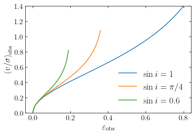
As expected, going from an edge-on to a face-on configuration increases the required \(v/\sigma\), because the intrinsic ellipticity is higher than the observed one for more face-on systems and this higher ellipticity requires higer \(v/\sigma\) to be supported. If elliptical galaxies are oblate, isotropic rotators, they should therefore lie above the blue line, with their exact predicted location depending on their inclinations.
We can compare these predictions to observations of \(v/\sigma\) and ellipticity for many elliptical galaxies, for example, the sample of galaxies from the integral-field surveys ATLAS\(^\mathrm{3D}\) and SAMI shown in the next figure:
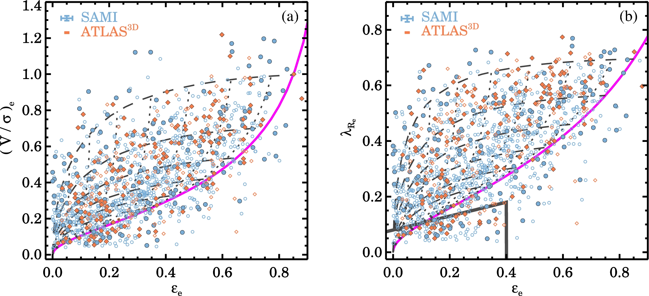
(Credit: van de Sande et al. 2017)
By comparing these observations to the curves in the previous figure, we see that many of the observed galaxies lie below the edge-on isotropic-rotator curve and almost all galaxies lie below the \(\sin i = \pi/4\) curve, which is the average inclination. Thus, most elliptical galaxies cannot be fully-isotropic rotators and anisotropy in the velocity dispersion must play a big role in the dynamical support of elliptical galaxies.
15.3. Schwarzschild modeling
Schwarzschild modeling is a powerful way to model the equilibrium structure of elliptical galaxies and triaxial mass distributions. While it is certainly possible to write down simple distribution function models for oblate elliptical galaxies much like we did for disk galaxies in Chapter 11, the complex orbital structure of many elliptical galaxies makes it difficult to create realistic models in this way. Moreover, coming up with simple triaxial models is difficult and only possible in very idealized cases. For this reason, it was unclear for a while after the first observational indications that many elliptical galaxies may be triaxial (which we discussed at the start of Chapter 13), whether stable, triaxial mass configurations are even possible in the first place. To resolve this question, Martin Schwarzschild developed a general, highly-flexible method for obtaining equilibrium models for very general mass distributions. In the 40 years since it appeared, this method has become widely used to study galactic equilibria and to interpret observational data.
The steady-state models for spherical and disk mass distributions that we have discussed in Chapters 6 and 11 have all been based on the Jeans theorem (Chapter 6.5): that any solution of the equilibrium collisionless Boltzmann equation only depends on the phase-space coordinates through the integrals of motion. Because of this theorem, we have built equilibrium models by positing that the distribution function is a function of one or more of the integrals of the motion (such as specific energy and specific angular momentum). We then either solved for such a function that corresponds to a given density profile (e.g., exactly for the case of the Eddington inversion for ergodic spherical systems of Chapter 6.6.1 or approximately for the disk distribution functions of Chapter 11.2.2) . Or we simply chose a form that seems reasonable and computed the resulting density distribution (like in the case of the isothermal sphere of Chapter 6.6.2). Another way of phrasing the Jeans theorem, however, is that the distribution function cannot depend on the phase along the orbit of a body, it can only change from orbit to orbit. Therefore, we can phrase the Jeans theorem in terms of orbits as
Orbit-based Jeans theorem: Any function that is constant along orbits is a solution of the equilibrium collisionless Boltzmann equation. Furthermore, any solution of the equilibrium collisionless Boltzmann equation is constant along orbits.
The first part of this theorem results from Liouville’s theorem (Equation 6.37): the distribution function does not change as a phase-space position orbits; therefore, if the distribution function is constant along the orbit at \(t=0\), it will be constant along the orbit at all times. The second part follows from the regular Jeans theorem: the regular Jeans theorem demonstrates that the distribution function is itself an integral of the motion; therefore, it is constant along orbits.
The orbit-based Jeans theorem therefore suggest another way of constructing equilibrium mass models: rather than positing a function of the integrals of motion (which are difficult to compute for general mass models), we can posit a function of the orbits themselves. This is a much more flexible way to create equilibrium mass models, because even when integrals of the motion are difficult to obtain (e.g., for a triaxial distribution), it is straightforward to numerically obtain orbits in any gravitational potential. This fundamental insight was first proposed by Schwarzschild (1979), who used it to obtain the first model for a triaxial stellar system in dynamical equilibrium (appropriately, the title of his paper!).
In this second part of the chapter, we discuss the general approach of Schwarzschild modeling, illustrate its use in a simple one-dimensional problem, and then discuss more detailed aspects of its application to full three-dimensional equilibrium models of real galaxies. Applications of Schwarzschild modeling are discussed further in Chapter 17.
15.3.1. General approach
Schwarzschild modeling was first used to create a dynamical model for a given general (e.g., triaxial) density distribution and we will describe this type of modeling first before describing how to incorporate constraints on the solution beyond the density. Given an equilibrium mass distribution \(\rho(\vec{x})\), we can obtain the gravitational potential \(\Phi(\vec{x})\) by solving the Poisson equation (e.g., for a triaxial system using the approach described in Chapter 13) . We then integrate a large number \(N\) of orbits \(i\) in this gravitational potential; each orbit is a time series of phase-space coordinates \(\vec{w}_i(t_k) = [\vec{x}_i(t_k),\vec{v}_i(t_k)]\) sampled at \(K\) regularly-spaced times \(t_k\). Given the time series, we can then determine each orbit’s contribution to the density at \(L\) points \(j\) \(\vec{x}_j\), for example, by making a histogram \(n_{ij}\) of the set of \(K\) \(\vec{x}_i(t_k)\) (approximating the density as the number of points \(k\) where \(\vec{x}_i(t_k)\) falls within a small volume \(\delta V_j\) around \(\vec{x}_ij\)).
We built a distribution function out of the \(N\) orbits by giving each orbit a weight \(w_i\); the total mass associated with a given orbit is then \(m_i = w_i\,M\), where \(M\) is the total mass of the galaxy. The total density at point \(\vec{x}_j\) corresponding to a set of weights \(w_i\) is then given by \(\tilde{\rho}_j = \sum_i w_i\,{n_{ij} \over K}\,{M \over\delta V_j}\). With \(p_{ij} \equiv n_{ij} / K\), the fraction of time an orbit spends in the volume near \(\vec{x}_j\), and \(\delta \rho_j \equiv M / \delta V_j\), the basic density discretization, this becomes
This model density can then be compared to the true density \(\rho(\vec{x}_j)\) and a perfect match is obtained when
For a given target density profile and a given set of orbits, this is a set of \(L\) linear equations in the unknown weights \(w_i\) that could be solved through standard techniques for solving linear sets of equations. In principle, it is therefore possible to use \(N = L\) orbits and solve this equation. However, a further constraint is necessary to obtain a physical distribution function, namely, that \(\forall i: w_i \geq 0\); all weights have to be positive or zero. This constraint will typically not be satisfied when \(N = L\): to exactly match the density at \(L\) points with \(L\) orbits, it will be necessary to include some negatively-weighted orbits and these are not physical configurations. It is therefore necessary to use \(N \gg L\) orbits, in which case the system of equations \(\eqref{eq-basic-schwarzschild-constraint}\) becomes underdetermined and an infinite \(N-L\) dimensional subspace of solutions is obtained. As long as this subspace overlaps with the part of space where \(\forall i: w_i \geq 0\), a physical solution is possible, but now we have infinitely many such solutions! To pick a specific solution requires specifying another constraint on the set of weights that corresponds to a desirable property of the solution: we specify some additional objective function \(S(\vec{w})\) that we want to maximize. Therefore, solving for the distribution function requires us to find the set of weights \(\vec{w} = w_i\) that solves
When the mass of the galaxy is known, an additional constraint is that \(\sum_i w_i = 1\).
While mass modeling of complex galactic distributions is a very esoteric subject, optimization problems of the sort \eqref{eq-schwarzschild-basicprogramming} are very commonly encountered throughout science and engineering and, in particular, in many business settings (for example, Fedex and other courier services need to solve instances of this problem daily to figure out the optimal delivery schedule for packages). Because of this, highly efficient open-source and commercial software packages exist to solve this class of problem (some quite pricey!) and even very large systems can be solved quickly. Depending on the form of the objective function. In general, the class of optimization problems \eqref{eq-schwarzschild-basicprogramming} is known as non-linear programming, with linear and quadratic programming corresponding to objective functions \(S(\vec{w})\) that are linear or quadratic, respectively, in the weights and for which special solution methods exist.
When Schwarzschild (1979) first proposed this method, he applied it to find a steady-state dynamical model for a triaxial version of a modified Hubble profile, which in the spherical case has \(\rho(r) \propto (1+r^2)^{-3/2}\). Because Schwarzschild only wanted to demonstrate the existence of any equilibrium distribution function for this triaxial system, he did not care greatly about the properties of the weights and therefore chose a simple linear objective function \(S(\vec{w})\), for which the solution of the problem \(\eqref{eq-schwarzschild-basicprogramming}\) is simple. However, using a linear objective function tends to lead to solutions with very spiky behavior, that is, where many weights are zero while only a small subset is non-zero, and the resulting distribution function is therefore not very smooth (and, thus, likely not very realistic for a real galaxy). The reason for this is that in many cases, minimizing a linear objective function over the weights is equivalent to minimizing the number of non-zero weights (Candes et al. 2006), an insight that has turned out to be highly productive in signal processing and many other modeling contexts (including in astrophysics), because it allows one to find solutions of underdetermined problems that are sparse in the number of coefficients (this field is known as “compressed sensing”, because it allows for significant compression of signals). However, for Schwarzschild modeling of galaxies, this is not a desirable property (an example is shown in the next section).
Non-linear objective functions are therefore preferred to create smoother distribution functions. Because quadratic objective functions lead to their own class of efficient solutions of the optimization problem \eqref{eq-schwarzschild-basicprogramming}, a quadratic objective function can be used. For example, \(S(\vec{w}) = -\sum_i w_i^2/W_i\) (optimizing this under the constraint \(\sum_i w_i = 1\) for a galaxy with known mass leads to \(w_i \propto W_i\) and the \(W_i\) are therefore a sort of prior assumption about what the weights should be). A popular, but fully non-linear objective function is the entropy, \(S(\vec{w}) = -\sum_i w_i\,\ln w_i\), which will tend to create smoother distribution functions. However, fully non-linear programming problems are harder to solve. An example of this is also shown below.
So far, we have only required that the density resulting from the weighted combination of orbits reproduces a target density. However, we can also incorporate constraints on the velocity structure of the model, because we have access to the velocities along each orbit. We can use the velocities, for example, to compute the mean velocity or the velocity dispersion in a volume around \(\vec{x}_j\), using moments computed using the orbit weights. For instance, we could attempt to create a model that is as close to isotropy as possible by including an objective function of the form
with the velocity dispersions computed at a set of points \(\vec{x}_l\), because minimizing this function would minimize differences between the velocity dispersions (the first term is the anisotropy for spherical systems that we defined in Equation 6.51). Similar objective functions could be used to obtain a certain anisotropy profile, to add overall rotation to the model, or to include constraints on higher-order moments of the velocity distribution. Because these are highly non-linear objective functions, solving the optimization problem becomes harder.
A second class of velocity constraints comes is observational. When Schwarzschild modeling is used to interpret observational data on the surface density and velocity structure of galaxies, the model’s velocity structure is matched to the observed structure using a chi-squared or likelihood-based objective function, \(S(\vec{w}) = -\chi^2\) or \(S(\vec{w}) = \ln \mathcal{L}\), where \(\chi^2\) or \(\ln \mathcal{L}\) is an expression that depends on the exact data obtained and its uncertainties. We discuss this in more detail in Section 15.3.3 below.
15.3.2. A worked example in one dimension
To illustrate the general concept of Schwarzschild modeling and its main ingredients, and to demonstrate how well it works, we apply it in this section to a simple one-dimensional problem. In particular, we consider the problem of determining the equilibrium distribution function of a constant density slab of matter, for which the gravitational potential is that of a harmonic oscillator. This makes for a great example, because orbit integration in this potential is analytic (see, e.g., Chapter 5.2.1) . As for any one-dimensional system, the correct distribution function for this density profile is easy to compute analytically (see Chapter 11.4.3 and below) and we can therefore straightforwardly check whether Schwarzschild modeling recovers the correct distribution function. Because the system is only one-dimensional, in practice running the Schwarzschild modeling procedure is very fast and can easily be done on any modern computer. However, keep in mind that one-dimensional modeling differs qualitatively from three-dimensional modeling, in that many of the practical issues with Schwarzschild modeling in three dimensional systems that we will discuss below, do not occur in one dimension or are easy to solve (such as, finding all the orbits, deciding how long to integrate, chaotic orbits, etc.).
We consider orbits in a one-dimensional harmonic-oscillator potential
where \(\omega\) is the frequency of the oscillator. All orbits in this potential are analytic and given by
where \(A_0\) and \(\phi_0\) are the amplitude and initial phase of the orbit that are given by the initial conditions. The amplitude \(A_0\) is related to the specific energy as
Thus, an orbit with specific energy \(E=0\) remains motionless at the bottom of the potential well and all non-trivial orbits have positive, non-zero specific energy and a period of \(T = 2\pi/\omega\). Orbits are labeled by \(A_0\) or, equivalently, \(E\) and form a one-dimensional sequence, as expected. By applying the Poisson equation, it is easy to see that a harmonic-oscillator potential corresponds to a constant density, with the relation between the constant density \(\rho_0\) and the oscillation frequency given by
Our goal is to find a self-consistent phase-space distribution function that produces a finite-width, constant density slab. That is, we want to find the distribution function that creates the density
where \(T\) is the thickness of the slab centered around \(x=0\). This problem can be solved analytically using the tools described in Chapter 11.4, and we will do that below, but let us determine this distribution using Schwarzschild modeling. We first implement a function that returns an entire orbit for a given specific energy \(E\), frequency \(\omega\), and number of times along the orbit:
[166]:
def harmOsc_orbit(E,omega,nt=101):
    """Return the orbit with specific energy E covering a single
    period of the harmonic oscillator potential with frequency omega;
    nt= number times along the orbit to return"""
    A0= numpy.sqrt(2.*E)/omega
    # Make sure not to double count t=0,period
    ts= numpy.linspace(0.,2*numpy.pi/omega,nt+1)[:-1]
    return (A0*numpy.cos(omega*ts),-A0*omega*numpy.sin(omega*ts))
To test this function, we plot the orbit with \(E=0.1\) in a potential with \(\omega=1.1\):
[167]:
plot(*harmOsc_orbit(0.1,1.1))
xlabel(r'$x$')
ylabel(r'$y$');
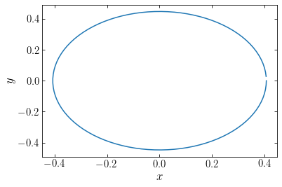
This orbit is the expected ellipse. Note that the plotted orbit doesn’t close, because in anticipation of using this function in Schwarzschild modeling, we have made sure to not have points along the orbit at the same orbital phase. Such points would be double-counted in using this orbit as a building block for the distribution function.
In Schwarzschild modeling we build the distribution function by weighting orbits such as the one that are used as building blocks of the galaxy. Uniformly sampling along the orbit above gives its contribution to the total density. The more points along the orbit that we evaluate, the better we approximate the orbit’s contribution to the total density. Here we compute an orbit’s contribution to the density simply by building a histogram of the orbit’s \(x\) values:
[168]:
hist(harmOsc_orbit(0.1,1.1)[0],bins=21,
     density=True,histtype='step')
hist(harmOsc_orbit(0.1,1.1,nt=1001)[0],bins=21,
     density=True,histtype='step')
xlabel(r'$x$');
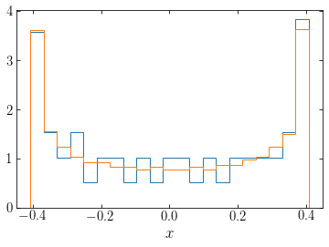
The orange curve uses ten times more points along the orbit than the blue curve and, as a result, it much smoother.
Combining the contributions of different orbits, we can build up the total density. As an example, we plot the contribution to the density from orbits with \(E=0.1, 0.2\) and \(0.3\) weighted equally:
[169]:
hist(numpy.array([harmOsc_orbit(0.1,1.1,nt=1001)[0]]).flatten(),
                  bins=21,histtype='step')
hist(numpy.array([harmOsc_orbit(0.1,1.1,nt=1001)[0],
                  harmOsc_orbit(0.2,1.1,nt=1001)[0]]).flatten(),
                  bins=21,histtype='step')
hist(numpy.array([harmOsc_orbit(0.1,1.1,nt=1001)[0],
                  harmOsc_orbit(0.2,1.1,nt=1001)[0],
                  harmOsc_orbit(0.3,1.1,nt=1001)[0]]).flatten(),
                  bins=21,histtype='step',lw=2.)
xlabel(r'$x$');
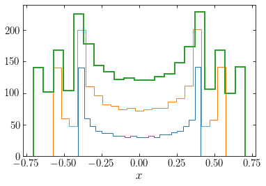
Each additional curve above the previous one shows the addition of one orbit, starting with the lowest specific energy one. We can write a general function that computes the total density for a set of orbits with energies \(\vec{E}\) and weights \(\vec{w}\):
[170]:
def harmOsc_dens(E,w,omega,nt=101,
                range=[-2.5,2.5],bins=51):
    """Return the combined density from orbits with
    specific energies E and weights w, with individual
    orbits sampled at nt times; compute the density as
    a histogram over 'range' in 'bins' bins"""
    return numpy.histogram(numpy.array([harmOsc_orbit(Ei,omega,nt=nt)[0]
                                        for Ei in E]).flatten(),
                           weights=numpy.tile(w,(nt,1)).T.flatten()
                                       *bins/(range[1]-range[0])/nt,
                           range=range,bins=bins)
For example, the total density if we weight all orbits with energies \(0 \leq E \leq 1\) equally is:
[171]:
hy,hx= harmOsc_dens(numpy.linspace(1e-10,1.,101),
                    numpy.ones(101)/101,1.1)
plot((numpy.roll(hx,-1)+hx)[:-1]/2.,hy,ds='steps-mid')
xlabel(r'$x$');
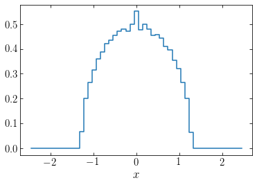
We now want to set the weights \(\vec{w}\) such that the resulting density distribution is that which sources the gravitational potential, that is, a constant density over the slab as in Equation \(\eqref{eq-slab-density}\). For this we will evaluate the density corresponding to a given orbit sampling represented by a set of energies \(\vec{E}\) and a set of orbit weights \(\vec{w}\) in bins like above and require that the density in each bin equals that of \(\eqref{eq-slab-density}\); that is, the resulting density should equal \(\rho_0\) within the slab and be zero outside. The only constraint on the weights is that they are positive, \(w_i \geq 0\,\forall i\).
To get a first sense of how this works, consider the interactive example below. On the left, you see a histogram of orbit weights for 10 energies spanning 0 to the maximum specific energy orbit. On the right, you see the resulting density histogram from combining all of the 10 orbits’ \(x\) values using their orbit weights. You can drag the top of the weight bins to change the orbit weights and watch how the resulting density changes. Try finding the combination of orbit weights that gives the correct constant density, given as the orange line!
To obtain a first quantitative solution, we follow the original procedure used by Schwarzschild (1979) and use the linear programming version of the optimization problem \eqref{eq-schwarzschild-basicprogramming}. However, the basic Schwarzschild modeling problem, of matching the density (Equation \ref{eq-basic-schwarzschild-constraint}) with positive weights, does not have a linear-programming loss function directly associated with it, so following
Schwarzschild, we can make up one at random. So to obtain a first solution, we will simply use the objective function \(\phi(\vec{w}) = \sum_i w_i\). We can solve the linear-programming problem using scipy.optimize’s linprog function, which allows one to solve very general linear-programming problems. The following function sets up the constraints in a way that linprog understands and then returns the result. We define the weights such that each orbit’s weight is the total mass
contributed by the orbit. Note that we do not enforce that the total mass of all the orbits is the known total mass of the system, as is commonly done in Schwarzschild modeling.
[172]:
from scipy import optimize
def optimize_weights_linprog(E,omega,nt=101,T=3.,
                            range=[-2.5,2.5],bins=51):
    """Determine the Schwarzschild modeling solution using
    linear programming using orbits with specific energies E,
    in a harmonic oscillator with frequency omega for a target
    slab with thickness T. Compute the model density as a
    histogram over 'range' in 'bins' bins.
    Returns the optimal weights of the orbits"""
    rho0= omega**2./(4.*numpy.pi)
    # Define constraints, integrate all orbits
    orbs= numpy.array([harmOsc_orbit(Ei,omega,nt=nt)[0] for Ei in E])
    # Compute density for each orbit
    orbhists= numpy.apply_along_axis(\
                lambda x: numpy.histogram(x,range=range,bins=bins,
                                          density=True)[0],1,orbs).T
    # orbhists is now the matrix A in the constraint equation
    # Density to match:
    dens_match= rho0*numpy.ones(bins)
    xbins= (numpy.roll(numpy.linspace(range[0],range[1],bins+1),-1)
            +numpy.linspace(range[0],range[1],bins+1))[:-1]/2.
    dens_match[(xbins < -T/2.)+(xbins > T/2)]= 0.
    # dens_match is now the vector b in the constraint equation
    # Random objective function: minimize sum of weights
    c= numpy.ones(len(E))
    # default in linprog is for all parameters to be positive,
    # so don't need to specify that
    return optimize.linprog(c,A_eq=orbhists,b_eq=dens_match)
We run the code for an example where \(\omega = 1.1\) and \(T = 3\). We attempt to match the density over the range \([-1.75,1.75]\) (the density should only be non-zero over \([-1.5,1.5]\) in this case, for \(T=3\)) using orbits with energies up to 120% of what we know the maximum specific energy to be, because the maximum specific energy is for an orbit that turns around at \(x = T/2\): \(E_{\mathrm{max}} = \omega^2 T^2/8\). We use 1001 orbits, evaluating 3001 points along each orbit to get an accurate sampling of the density contributed by each orbit:
[173]:
omega= 1.1
T= 3.
Emax= omega**2.*T**2./8.
xrange= [-1.75,1.75]
nE= 1001
nt= 3001
bins= 101
E= numpy.linspace(0.,Emax*1.2,nE)
dE= E[1]-E[0]
opt= optimize_weights_linprog(E,omega,T=T,
                              bins=bins,range=xrange,nt=nt)
The weights specify how much mass is contributed to the system by orbits with different energies. In the following, we plot the differential specific energy distribution \(N(E)\), which is the amount of mass per unit specific energy:
[174]:
plot(E,opt['x']/dE)
xlabel(r'$E$')
ylabel(r'$N(E)$');
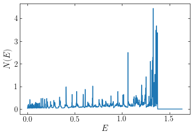
We see that the distribution of energies is very spiky, with only a few orbits dominating the distribution. This is because we chose a loss function that does not penalize non-smooth distribution and that in fact maximizes spikiness (see the discussion in the previous section). Nevertheless, the density distribution resulting from this set of weights matches the target density very well:
[175]:
hy,hx= harmOsc_dens(E,opt['x'],omega,nt=nt,range=xrange)
plot((numpy.roll(hx,-1)+hx)[:-1]/2.,hy,ds='steps-mid')
plot(numpy.linspace(-T/2,T/2,101),
     omega**2./(4.*numpy.pi)*numpy.ones(101))
ylim(0.,omega**2./(4.*numpy.pi)*1.5)
xlabel(r'$x$');
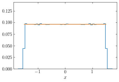
The target density is shown in orange over the range where it is non-zero and as we can see, the density distribution corresponding to the optimized weights (blue curve) matches this constant density and its range very well. The non-smoothness of the weight distribution is such that if we slightly change the set of orbits used, we can get quite different weights for orbits that are otherwise similar. For example, in the following, we use 2001 orbits using a slightly different specific energy sampling:
[176]:
omega= 1.1
T= 3.
Emax= omega**2.*T**2./8.
xrange= [-1.75,1.75]
nE= 2001
nt= 3001
bins= 101
E2= numpy.linspace(0,Emax*1.1,nE)
dE2= E2[1]-E2[0]
opt2= optimize_weights_linprog(E2,omega,T=T,
                               bins=bins,range=xrange,nt=nt)
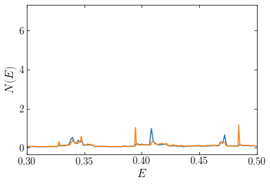
Comparing the differential specific energy distribution, we see overall okay agreement:
[177]:
plot(E,opt['x']/dE)
plot(E2,opt2['x']/dE2)
xlabel(r'$E$')
ylabel(r'$N(E)$');
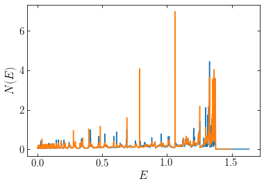
but zooming in, we see that the spikes in the weight distribution can be quite different heights:
[178]:
plot(E,opt['x']/dE)
plot(E2,opt2['x']/dE2)
xlim(0.3,.5)
xlabel(r'$E$')
ylabel(r'$N(E)$');
To obtain a smoother, and thus more realistic distribution, we need to use a loss function that penalizes non-smoothness. For the sake of this demonstration, we will use the entropy loss function and make use of scipy’s constrained optimization routines. The following function implements the entropy loss function and collects the constraints on the weights in a way that they can be given to the scipy.optimize.minimize function:
[179]:
from scipy import optimize
def optimize_weights_entropy(E,omega,nt=101,T=3.,
                             range=[-2.5,2.5],bins=51):
    rho0= omega**2./(4.*numpy.pi)
    # Initial value
    init_w= numpy.ones_like(E)/len(E)
    # Define loss function and its Jacobian: minimize minus the entropy
    def loss(w):
        return numpy.sum(w*numpy.log(w))
    def jac(w):
        return numpy.log(w)+1.
    # Define the constraint equation:
    # Integrate all orbits
    orbs= numpy.array([harmOsc_orbit(Ei,omega,nt=nt)[0] for Ei in E])
    # Compute density for each orbit
    orbhists= numpy.apply_along_axis(\
                    lambda x: numpy.histogram(x,range=range,bins=bins,
                                              density=True)[0],1,orbs).T
    # Density to match:
    dens_match= rho0*numpy.ones(bins)
    xbins= (numpy.roll(numpy.linspace(range[0],range[1],bins+1),-1)
            +numpy.linspace(range[0],range[1],bins+1))[:-1]/2.
    dens_match[(xbins < -T/2.)+(xbins > T/2)]= 0.
    constraints= [{'type':'eq',
                   'fun':lambda w: numpy.dot(orbhists,w)-dens_match,
                   'jac':lambda w: orbhists},
                  {'type':'ineq',
                   'fun': lambda w: w}]
    return optimize.minimize(loss,
                             numpy.copy(init_w)\
                                 *(1.+numpy.random.normal(size=len(init_w))/10.),
                             jac=jac,constraints=constraints,
                             method='SLSQP',options={'maxiter':1001})
We apply this method to the same problem as above, now using only 201 orbits for 31 density bins. Constrained, non-linear optimization is a difficult problem and going to larger numbers of bins fails to produce a solution in this case, but the setup below should work:
[180]:
omega= 1.1
T= 3.
Emax= omega**2.*T**2./8.
xrange= [-1.75,1.75]
nE= 201
nt= 3001
bins= 31
E_ent= numpy.linspace(1e-10,Emax*1.2,nE)
dE_ent= E_ent[1]-E_ent[0]
opt_ent= optimize_weights_entropy(E_ent,omega,T=T,
                                  bins=bins,range=xrange,nt=nt)
We now again plot the differential specific energy distribution and it looks much smoother than before:
[181]:
plot(E_ent,opt_ent['x']/dE_ent,
     label=r'$\mathrm{entropy}$',zorder=2,lw=2.)
plot(E,opt['x']/dE,label=r'$\mathrm{linear}$',zorder=1)
xlabel(r'$E$')
ylabel(r'$f(E)$')
legend(fontsize=18,frameon=False);
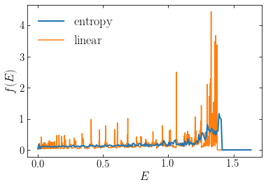
We see that the entropy-based solution is much less spiky than the solution using the linear loss function that we obtained above. The match of the density corresponding to the orbital weights with the target density is equally good as above:
[182]:
hy,hx= harmOsc_dens(E_ent,opt_ent['x'],omega,
                    nt=nt,range=xrange)
plot((numpy.roll(hx,-1)+hx)[:-1]/2.,hy,
     ds='steps-mid',label=r'$\mathrm{entropy}$',
     zorder=2,lw=2.)
hy,hx= harmOsc_dens(E,opt['x'],omega,
                    nt=nt,range=xrange)
plot((numpy.roll(hx,-1)+hx)[:-1]/2.,hy,
     ds='steps-mid',label=r'$\mathrm{linear}$',
     zorder=1)
plot(numpy.linspace(-T/2,T/2,101),
     omega**2./(4.*numpy.pi)*numpy.ones(101))
ylim(0.,omega**2./(4.*numpy.pi)*1.5)
xlabel(r'$x$')
legend(fontsize=18,frameon=False);
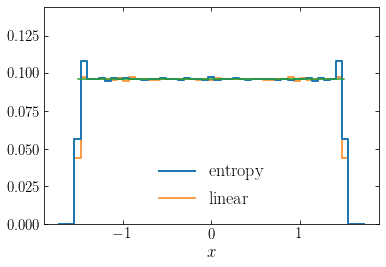
Thus, both are good solution, but the entropy one is obviously to be preferred as it is smoother.
Because we can compute the steady-state distribution function for a one-dimensional system directly, we can compare the numerical solution above to the true solution. To compute the homogeneous slab’s equilibrium distribution function directly, we use the approach from Chapter 11.4.3. There we derived that the equilibrium distribution function \(f(E)\) corresponding to a given density proflie \(\nu(x)\) in a potential \(\Phi(x\)) is given by
To apply this equation, we require the derivative of the density with respect to the potential. Because the density is everywhere constant, except where it drops to zero at the edge of the slab, it is clear that we have to have that
because the derivative of the unit step function is the delta function. Plugging this into Equation \(\eqref{eq-oned-eq-df-abel}\), we can work out that
Defining
we can also write this as
Using the Poisson equation for the slab \(\eqref{eq-slab-poisson}\), we can also relate the thickness \(T\) to \(\sigma\) as
We define a function that computes \(f(E)\) for a given \(\omega\), \(T\), and \(\rho_0\).
[183]:
def harmOsc_df_analytic(E,omega,T=3.):
    """Equilibrium distribution function for a harmonic
    oscillator with frequency omega and a constant-density
    slab of thickness T as a function of specific energy E."""
    sigma2= omega**2.*T**2./8.
    rho0= omega**2./(4.*numpy.pi)
    out= rho0/numpy.sqrt(2*sigma2*(1.-E/sigma2))/numpy.pi
    out[E >= sigma2]= 0.
    return out
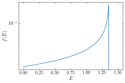
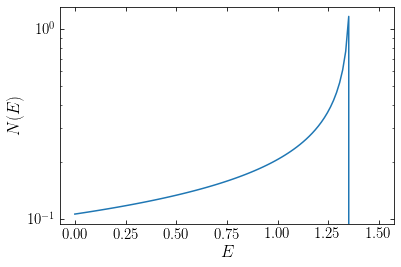
The distribution function \(f(E)\) looks as follows:
[184]:
Es= numpy.linspace(1e-10,1.5,101)
semilogy(Es,harmOsc_df_analytic(Es,omega))
xlabel(r'$E$')
ylabel(r'$f(E)$');
However, we cannot directly compare this \(f(E)\) to the orbital weights, because \(f(E)\) gives the value of the distribution function at a given \((x,v)\), which in a steady state is only a function of integrals of the motion like the specific energy. That is, \(f(E)\) is the value of the probability distribution \(f(x,v)\) rather than a probability distribution in specific-energy space itself, which is what the distribution of orbital weights is (see the discussion in Chapter 6.5). To get the theoretical differential specific-energy distribution \(N(E)\), we need to multiply \(f(E)\) with the volume of phase-space \(g(E)\) occupied by orbits with specific energy \(E\). This function \(g(E)\) is called the density of states and it can be computed as
where \(H[x,v]\) is the Hamiltonian. For the harmonic oscillator with non-zero density over the slab with width \(T\), this becomes
where we have used the transformations \(\xi = v^2/2\) and \(y = \omega x / \sqrt{2E}\) to simplify the integrals. Thus, we see that for the one-dimensional harmonic oscillator potential, the density of states is actually a constant equal to the period of the orbit. For the sake of generality, we nevertheless implement a function that returns the density of states \(g(E) = 2\pi/\omega\):
[185]:
def harmOsc_density_states(E,omega,T=3.):
    """The density of states for a harmonic
    oscillator with frequency omega over a
    constant-density slab with thickness T
    as a function of the specific energy E"""
    return 2.*numpy.pi/omega*numpy.ones_like(E)
The theoretically expected differential specific-energy distribution for the one-dimensional slab is therefore given by:
[186]:
Es= numpy.linspace(1e-10,1.5,101)
semilogy(Es,harmOsc_df_analytic(Es,omega)*harmOsc_density_states(Es,omega))
xlabel(r'$E$')
ylabel(r'$N(E)$');
Now we can compare the expected differential specific-energy distribution with the one obtained by optimizing the orbital weights using Schwarzschild modeling:
[187]:
plot(E_ent,opt_ent['x']/dE_ent)
plot(Es,harmOsc_df_analytic(Es,omega,T=T)
         *harmOsc_density_states(Es,omega))
xlabel(r'$E$')
ylabel(r'$N(E)$');
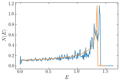
We see that the agreement is excellent: the shape and amplitude of the differential specific-energy distributions almost exactly matches. The Schwarzschild-modeled weights extend to somewhat larger energies, which is because of the coarse density grid that we employed when matching the density, but otherwise the two functions are very similar. Schwarzschild modeling with a loss function that penalizes spiky distribution functions therefore returns the correct distribution function for this one-dimensional system.
15.3.3. Studying observed galaxies using Schwarzschild modeling
The one-dimensional example above is useful for showing how Schwarzschild modeling works in principle and in demonstrating that it recovers the correct distribution function. But being in one dimension, it is a highly idealized example that does not suffer from the complexities that plague three-dimensional Schwarzschild modeling (including such seemingly simple questions as “How long should I integrate orbits for?”). It also does not illustrate how Schwarzschild modeling is used for building dynamical models of observed galaxy photometry and kinematics. This section provides an introduction into the practice of Schwarzschild modeling of observed, external galaxies.
Observational Schwarzschild modeling generally proceeds in the manner schematically shown in the following flowchart from Cretton et al. (1999):
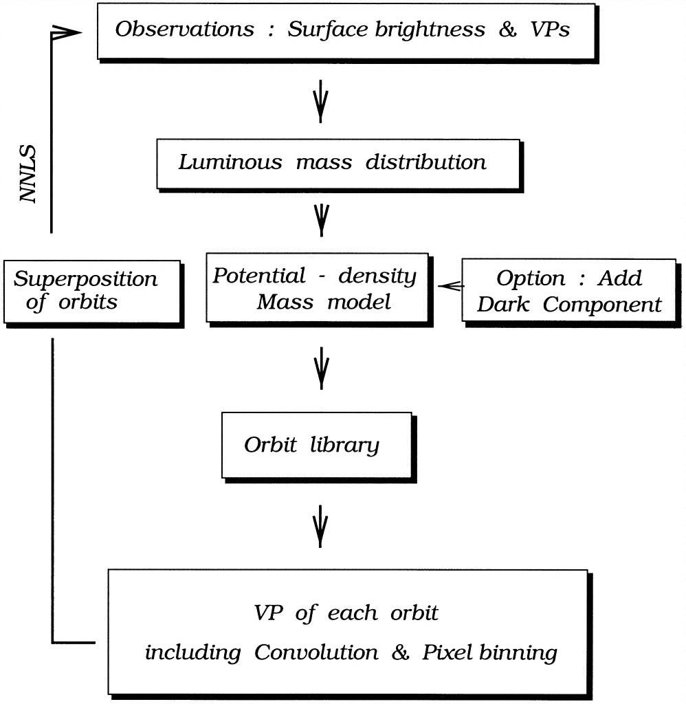
(Credit: Cretton et al. 1999)
At the top of this flowchart are the typical observables available for observational Schwarzschild modeling: photometric measurements of the surface brightness of the galaxy and information on the velocity distribution (“velocity profile”; VP) in the galaxy. This velocity information typically exists in the form of constraints on the moments of the line-of-sight velocity distribution obtained from long-slit spectroscopy along the major and minor axis of the galaxy (e.g., Franx et al. 1989; Bender et al. 1994) or, nowadays, from integral-field spectroscopy (IFS) over a two-dimensional area with various ground-based instruments (e.g., SAURON: Bacon et al. 2001; MUSE: Bacon et al. 2010). The extracted moments typically go up to the fourth moment: mean velocity, velocity dispersion, and the third and fourth moments expressed as Gauss-Hermite moments \(h_3\) and \(h_4\) (van der Marel & Franx 1993); however, the details of this do not concern us here.
Rather than blindly proposing mass models, using them to integrate orbits, and match the observed surface brightness and kinematic information (which would be extremely expensive to do!), the observed surface brightness is used to build a mass model for the luminous component(s) of the galaxy. Because the surface brightness corresponds to the two-dimensional projection of the underlying, three-dimensional luminosity density, assumptions about the underlying density have to be made in order to deproject it, and values for the orientation of the galaxy with respect to the line of sight need to be chosen (the inclination, but for triaxial models there is an additional angle as well). We discuss this deprojection further below. Next, one has to convert luminosity (“light”) to mass, which is generally done by assuming a constant mass-to-light ratio \(M/L\), although this could depend on position in the galaxy or vary between different components; this conversion then gives a mass model for the luminous component. To this one can add dark components—in elliptical galaxies either a dark-matter halo or a central, supermassive black hole—to obtain the full gravitational potential.
Once one has a model for the full gravitational potential, this potential is then used to create an orbit library that contains the building blocks (the orbits) of a Schwarzschild model. For a given set of orbit weights, one can then predict both the surface brightness and whatever kinematic information is available (e.g., the mean velocity and velocity dispersion profile along the major axis, or over the face of the galaxy for IFS data), and the weights are optimized using non-linear programming (Equation \ref{eq-schwarzschild-basicprogramming}), with the the equality constraint corresponding to the requirement that the dynamical model should match the input luminous mass profile and the kinematic information included as a minus-chi-squared (or log likelihood) contribution to the objective function to be maximized. By running many instances of this basic Schwarzschild modeling procedure for different settings of the assumed parameters (inclination, mass-to-light ratio[s], mass of a supermassive black hole, properties of the dark-matter halo, etc.) and comparing the objective function for the best-fit orbital-weight distribution for each model, one can determine the overall best model.
This is a complicated procedure! And what’s worse, each individual part of it has its own set of complexities that make them highly non-trivial. So let’s walk through some of the steps in more detail in the context of a real, observed galaxy (but we won’t attempt to do the full Schwarzschild modeling, that would take us too long!). As the example, we consider NGC 4342, a low-luminosity lenticular galaxy in the Virgo cluster that has a supermassive black hole at its center (Cretton & van den Bosch 1999). The following images from SDSS and HST observations show what NGC 4342 looks like:
|
|
|
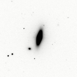
(Credit: SDSS \(i\) image from Baillard et al. 2011; HST WFPC2/F814W images [middle, zoomed on the right] from Cappellari 2002)
It is clear that NGC 4342 has a complex structure: as can be seen in the HST image, the isophotes are strongly flattened in the inner arcsecond, indicating the presence of a nuclear disk. A popular semi-parametric—meaning a model that has so many parameters that it is highly flexible—method for fitting the surface brightness profile and deprojecting it to a three-dimensional profile is that of a multi-Gaussian expansion (MGE). Such a model is easy to deal with: it can be de-projected straightforwardly under various assumptions about the underlying three-dimensional density (axisymmetric, or triaxial) and the gravitational potential can be easily computed using the methods of Chapter 13.2 (Emsellem et al. 1994). Efficient algorithms also exist to fit the MGE to observed surface photometry (Cappellari 2002; Shajib 2019).
Using similar notation as in Chapter 9.1.2, in the MGE, the observed surface brightness (in linear units of, e.g., \(L_\odot\,\mathrm{pc}^{-2}\)) \(\Sigma(r,\phi)\) is decomposed into \(N\) Gaussians as
where \((x'_j,y'_j)\) is the rectangular coordinate system on the sky in which the major axis falls along the \(x'_j\) axis
The parameters \((L_j,\sigma'_j,q'_j,\psi'_j)\) characterize each Gaussian: they are the total luminosity, the dispersion (in angular units) along the major axis, the axis ratio \(q'_j \leq 1\), and the position angle \(\psi'_j\); we use primed variables to indicate those that are specific to the sky projection. When not all \(\psi'_j\) are equal, then the galaxy has to be triaxial (this indicates the isophote twists discussed in Chapter 13) . The MGE surface brightness can be deprojected to a three-dimensional Gaussian expansion of the luminosity density (again working on coordinates aligned with the major axes)
The \(p_j\) parameters are necessary when the deprojection is triaxial (necessary when not all \(\psi'_j\) are equal), but to keep things simple, we will only consider axisymmetric deprojections, with \(p_j = 1\). The only angle necessary for the deprojection is then the inclination \(i\) (defined such that an inclination of \(i = 90^\circ\) indicates an edge-on galaxy) and we have that
for an oblate deprojection and \(q_j = \sqrt{\sin^2 i / (1/q'^2_j - \cos^2 i)}\) for a prolate deprojection. See Cappellari (2002) for expressions for triaxial deprojections. The mass density \(\rho(x,y,z)\) can then be obtained by multiplying the luminosity density \(j(x,y,z)\) from Equation \eqref{eq-mge-3dlumdens} by the mass-to-light ratio \(M/L\) (which could be taken to be different for different Gaussians without complicating the calculation of the gravitational potential).
We will use the decomposition obtained using the code of Cappellari (2002) to fit the HST images shown above, to create a three-dimensional model of NGC 4342. Note that NGC 4342 is conveniently oriented almost edge-on and an axisymmetric deprojection is therefore almost unambiguous. The output from the Cappellari (2002) code is the total number of counts (as the Gaussians are fit to the raw photon count map), standard deviation in pixel units, and the flattening of the profile for each Gaussian. We load the output from the code in the following cell:
[2]:
ngc4342_counts= numpy.array([8656.99,29881.7,134271,48555.8,266390,
                             258099,138127,346805,103864,894409,
                             742665,266803])
ngc4342_sigpix= numpy.array([0.605197,2.12643,6.43766,7.38899,13.3541,
                             24.5162,44.5134,57.7564,86.9258,144.783,
                             260.711,260.711])
ngc4342_qprojs= numpy.array([0.805036,0.896834,0.713238,0.178244,
                             0.758412,0.878234,1,0.366929,1,0.26115,
                             0.294149,0.677718])
ngc4342_pixscale= 0.0455 # arcsec/pixel
ngc4342_exptime= 200 # s exposure time
ngc4342_distance= 16.*u.Mpc
ngc4342_inclination= 83.*u.degree
ngc4342_sky_pa= 35.8*u.degree
ngc4342_extinction= 0.031 # from NED
where we have also defined the pixel scale for the HST WFPC2/F814W observations used in the fit and the exposure time of the image (200 seconds), and we have assumed a value for the distance, inclination (almost edge-on, but not exactly to keep things more interesting), the position angle on the sky, and extinction. We can then convert these counts to the total surface brightness in \(L_\odot\,\mathrm{pc}^{-2}\), luminosity in \(L_\odot\), and after assuming a mass-to-light ration, mass in \(M_\odot\). The details of this transformation are somewhat complex and specific to the HST WFPC2/F814W observations, so we simply use them here without providing further details and obtain the total mass associated with each Gaussian component:
[3]:
def counts_to_surfdens(counts,sigpix,qproj,
                       pixscale,exptime,distance,
                       extinction=0.):
    C0= counts/(2.*numpy.pi*sigpix**2.*qproj)
    surfbright= 20.84+0.1+5.*numpy.log10(pixscale)\
        +2.5*numpy.log10(exptime)-2.5*numpy.log10(C0)-extinction
    return (64800./numpy.pi)**2.*10.**(0.4*(4.08-surfbright))*u.Lsun/u.pc**2.
def counts_to_luminosity(counts,sigpix,qproj,
                         pixscale,exptime,distance,
                         extinction=0.):
    surfdens= counts_to_surfdens(counts,sigpix,qproj,
                                 pixscale,exptime,distance,
                                 extinction=extinction)
    return 2.*numpy.pi*surfdens\
        *(sigpix*pixscale*(u.arcsec/u.rad).to(u.dimensionless_unscaled)\
          *distance)**2.*qproj
ngc4342_ml= 4.*u.Msun/u.Lsun
ngc4342_masses= ngc4342_ml*counts_to_luminosity(ngc4342_counts,ngc4342_sigpix,
                                                ngc4342_qprojs,ngc4342_pixscale,
                                                ngc4342_exptime,ngc4342_distance,
                                                extinction=ngc4342_extinction)
We also implement and apply the deprojection of the axis ratio from Equation \eqref{eq-ellipequil-mge-qjdproject}:
[4]:
def qproj_to_q(qproj,inclination):
    return numpy.sqrt(qproj**2.-numpy.cos(inclination)**2.)/numpy.sin(inclination)
ngc4342_qs= qproj_to_q(ngc4342_qprojs,ngc4342_inclination)
and finally we compute the dispersion \(\sigma_j\) in physical units (of distance):
[5]:
ngc4342_sigmas= (ngc4342_sigpix*ngc4342_pixscale*u.arcsec*ngc4342_distance)\
    .to(u.kpc,equivalencies=u.dimensionless_angles())
We can then define a function that sets up a three-dimensional MGE model for a given set of parameters (we also allow it to rotate the model such that the \(x-y\) plane is parallel to the sky):
[6]:
from galpy.potential import TriaxialGaussianPotential
from galpy.util import _rotate_to_arbitrary_vector
def multi_gaussian_potential(masses,sigmas,qs,
                             inclination=None,sky_pa=None):
    """Set up an MGE mass model in galpy given a
    set of deprojected (masses,dispersions,axis ratios)
    Set the inclination and sky-position angle if you want
    to be able to show the model on the sky"""
    # Deal with inclination and sky position angle if given
    if not inclination is None:
        if sky_pa is None: sky_pa= 0.
        zvec_rot= numpy.dot(numpy.array([[numpy.sin(sky_pa),numpy.cos(sky_pa),0.],
                                         [-numpy.cos(sky_pa),numpy.sin(sky_pa),0.],
                                         [0.,0.,1]]),
                            numpy.array([[1.,0.,0.],
                                         [0.,-numpy.cos(inclination),-numpy.sin(inclination)],
                                         [0.,-numpy.sin(inclination),numpy.cos(inclination)]]))
        zvec= numpy.dot(zvec_rot,numpy.array([0.,0.,1.]))
        int_rot= _rotate_to_arbitrary_vector(numpy.array([[0.,0.,1.]]),
                                             zvec,inv=False)[0]
        pa= numpy.dot(int_rot,numpy.dot(zvec_rot,[1.,0.,0.]))
        pa= numpy.arctan2(pa[1],pa[0])
    else:
        zvec, pa= None, None
    # Now set up the sum of Gaussians, simply a list
    out= []
    for mass,sigma,q in zip(masses,sigmas,qs):
        out.append(TriaxialGaussianPotential(amp=mass,sigma=sigma,
                                             c=q.to_value(u.dimensionless_unscaled),
                                             zvec=zvec,pa=pa))
    return out
We first initialize a model rotated such that the \(z\) axis is the line-of-sight and such that the galaxy in the \(x-y\) plane should lie where the observed galaxy is:
[7]:
ngc4342_mge_pot_sky= multi_gaussian_potential(ngc4342_masses,
                                              ngc4342_sigmas,
                                              ngc4342_qs,
                                              inclination=ngc4342_inclination,
                                              sky_pa=ngc4342_sky_pa)
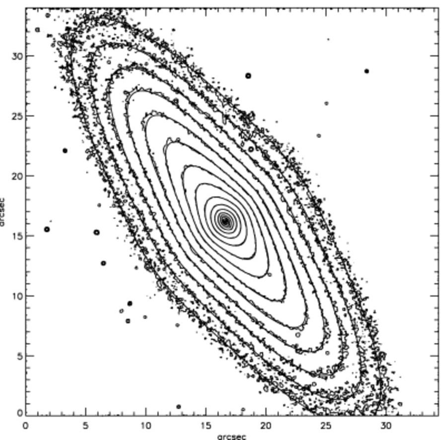
The surface density of the model over \(35^{\prime\prime}\) (similar to the middle panel above is):
[28]:
from galpy.potential import plotSurfaceDensities
figsize(5,5)
xmax= ((35./2.*u.arcsec)*ngc4342_distance).to(u.kpc,equivalencies=u.dimensionless_angles())
plotSurfaceDensities(ngc4342_mge_pot_sky,log=True,
                     xmin=-xmax,xmax=xmax,ymin=-xmax,ymax=xmax,
                     nxs=40,nys=40,
                     justcontours=True,ncontours=13)
gca().set_aspect('equal');
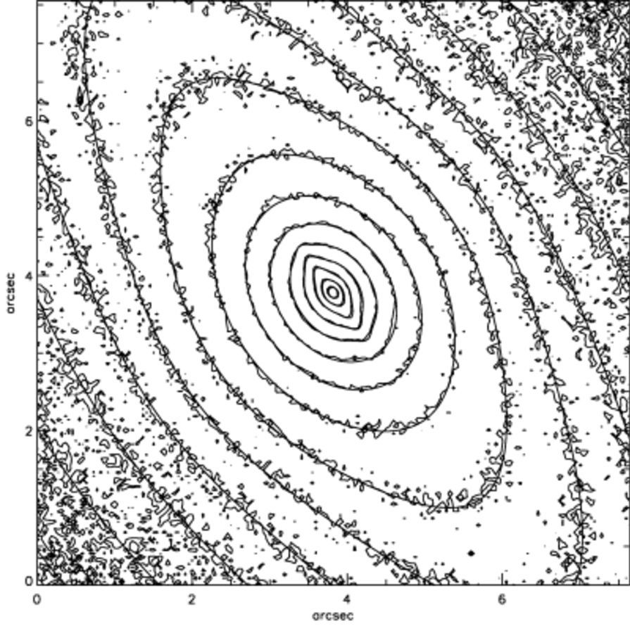
and zoomed in on the central \(\approx 7^{\prime\prime}\):
[29]:
from galpy.potential import plotSurfaceDensities
figsize(5,5)
xmax= ((7.5/2.*u.arcsec)*ngc4342_distance).to(u.kpc,equivalencies=u.dimensionless_angles())
plotSurfaceDensities(ngc4342_mge_pot_sky,log=True,
                     xmin=-xmax,xmax=xmax,ymin=-xmax,ymax=xmax,
                     nxs=40,nys=40,
                     justcontours=True,ncontours=13)
gca().set_aspect('equal');
where we see the narrowing of the isophotes near the center of the galaxy. Comparing these surface-density contours to the observations above, we can see that the model is a good match (the smooth contours in the observed pictures is approximately the same MGE). Now that we are happy with the model we set up a version that has the major and minor axes aligned with the coordinate axes:
[7]:
ngc4342_mge_pot= multi_gaussian_potential(ngc4342_masses,
                                              ngc4342_sigmas,
                                              ngc4342_qs)
Then we can, for example, plot the rotation curve in the inner kpc:
[8]:
from galpy.potential import plotRotcurve
figsize(5,5)
plotRotcurve(ngc4342_mge_pot,Rrange=[0.,1.*u.kpc]);
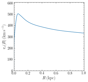
In building a Schwarzschild model of NGC4342, the next step is to integrate orbits in this potential (assuming that we do not need to add any additional dark component) and build an orbit library. To build an orbit library for an axisymmetric model, we can use the specific energy and the \(z\)-component of the specific angular momentum as two grid axes, because these are integrals of the motion. But as we saw in Chapter 14.1, most orbits in an axisymmetric potential have a third integral for which, however, no explicit expression is known. We therefore need a third dimension to build the full orbit grid, but there is no a priori obvious way to build this third dimension from an integral of motion.
One way to tackle this problem is to use the potential’s zero-velocity curve (see Chapter 10.1): the locus of points for a given \(E\) and \(L_z\) for which \(\Phi(R,z) + L_z^2/[2\,R^2] = E\) (equivalent to \(v_R = v_z = 0\)). This is a useful place to start, because almost all orbits intersect the zero-velocity curve in two points at \(z \geq 0\) (the thin tube orbit only has a single intersection point and certain periodic orbits do not intersect at all; Ollongren (1962)). For example, let’s consider orbits with specific energy equal to the specific energy of a circular orbit at \(500\) pc and \(z\)c-component of the specific angular momentum half of that of the circular orbit; we start orbits along the zero-velocity curve on a grid in \(R\) and plot their resulting surface of section (using our surface-of-section function from Chapter 14.1):
[59]:
from galpy.potential import (evaluatePotentials, vcirc,
                             zvc, zvc_range)
from galpy.orbit import Orbit
def surface_section(Rs,zs,vRs):
    # Find points where the orbit crosses z from - to +
    shiftzs= numpy.roll(zs,-1)
    indx= (zs[:-1] < 0.)*(shiftzs[:-1] > 0.)
    return (Rs[:-1][indx],vRs[:-1][indx])
def orbit_zvcELz(R,E,Lz,pot=None):
    """Returns Orbit initialized at zero-velocity curve at R with given (E,Lz)"""
    return Orbit([R,0.*u.km/u.s,Lz/R,zvc(pot,R,E,Lz),0.*u.km/u.s,0.*u.rad],ro=8.,vo=220.)
Rc= 500.*u.pc
E= evaluatePotentials(ngc4342_mge_pot,Rc,0.)+vcirc(ngc4342_mge_pot,Rc)**2./2.
Lz= Rc*vcirc(ngc4342_mge_pot,Rc)/2.
zvc_Rmin, zvc_Rmax= zvc_range(ngc4342_mge_pot,E,Lz)
ts= numpy.linspace(0.,1.,1001)
sect_ts= numpy.linspace(0.,100.,100001) # Longer for SOS
figsize(10,5)
orbs= []
for Rstart in numpy.linspace(zvc_Rmin*1.01,zvc_Rmax*0.99,5):
    o= orbit_zvcELz(Rstart,E,Lz,pot=ngc4342_mge_pot)
    o.integrate(ts,ngc4342_mge_pot)
    subplot(1,2,1)
    o.plot(gcf=True)
    subplot(1,2,2)
    o.integrate(sect_ts,ngc4342_mge_pot)
    sect1Rs,sect1vRs=surface_section(o.R(sect_ts),o.z(sect_ts),o.vR(sect_ts))
    plot(sect1Rs,sect1vRs,'o',mec='none')
    orbs.append(o)
subplot(1,2,1)
Rs= numpy.linspace(*zvc_range(ngc4342_mge_pot,E,Lz),101)
plot(Rs,numpy.array([zvc(ngc4342_mge_pot,R,E,Lz).to_value(u.kpc) for R in Rs])*u.kpc,
     color='k',lw=2.,zorder=0)
plot(Rs,-numpy.array([zvc(ngc4342_mge_pot,R,E,Lz).to_value(u.kpc) for R in Rs])*u.kpc,
     color='k',lw=2.,zorder=0)
subplot(1,2,2)
xlabel(r'$R\,(\mathrm{kpc})$')
ylabel(r'$v_R\,(\mathrm{km\,s}^{-1})$')
tight_layout();
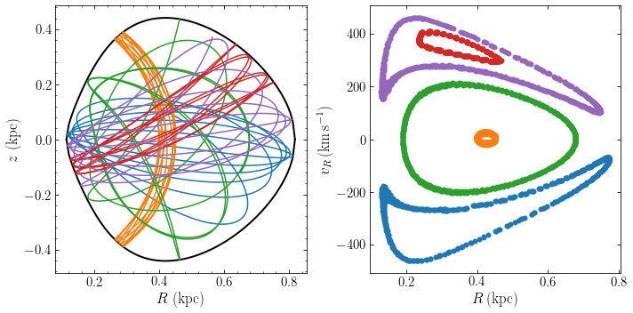
The left panel of the above figure shows a small part of the orbit (so the figure does not become too much of a mess), while the right shows the surface of section resulting from a long orbit integration. It’s clear that by simply scanning along the zero-velocity curve, we can efficiently explore the different types of orbits for a given specific energy and specific angular momentum (indeed, we immediately stumbled upon a bunch or resonant orbits and got close to the thin tube orbit).
We can then combine the orbits with weights and see what density distribution they lead to. For example, the orbits from above plotted in the \(x-z\) plane are
[98]:
figsize(11,4)
for ii,o in enumerate(orbs):
    subplot(1,len(orbs),ii+1)
    plot(o.x(sect_ts[:len(sect_ts)//20:10]),o.z(sect_ts[:len(sect_ts)//20:10]),
         '-',color=rcParams['axes.prop_cycle'].by_key()['color'][ii])
    xlim(-0.83,0.83)
    ylim(-0.49,0.49)
    xlabel(r'$x\,(\mathrm{kpc})$')
    if ii == 0: ylabel(r'$z\,(\mathrm{kpc})$')
    else: tick_params(axis='y',which='both',labelleft=False)
tight_layout();
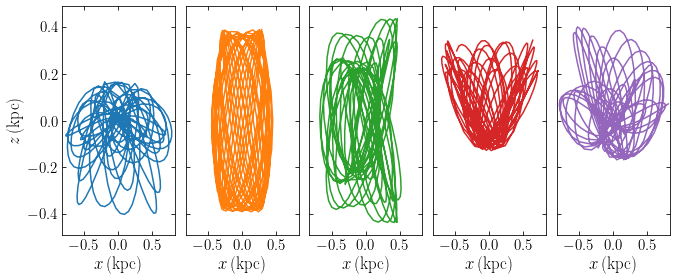
and we can, for example, predict the surface density by binning, e.g., using equal weighting of the orbits:
[60]:
orbital_weights= [1.,1.,1.,1.,1.]
hexbin(numpy.array([o.x(sect_ts) for o in orbs]).flatten(),
       numpy.array([o.z(sect_ts) for o in orbs]).flatten(),
       C=numpy.array([w*numpy.ones_like(o.x(sect_ts))
                      for (w,o) in zip(orbital_weights,orbs)]).flatten(),
       gridsize=31,reduce_C_function=numpy.sum)
colorbar()
xlabel(r'$x\,(\mathrm{kpc})$')
ylabel(r'$z\,(\mathrm{kpc})$');
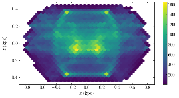
Like in the one-dimensional example from the previous section, we very much see the turning points of the individual orbits here. Attempting to get a flatter distribution by giving more weight to those orbits that remain closer to the \(x-y\) plane, we obtain
[61]:
orbital_weights= [1.,0.3,0.1,0.3,1.]
hexbin(numpy.array([o.x(sect_ts) for o in orbs]).flatten(),
       numpy.array([o.z(sect_ts) for o in orbs]).flatten(),
       C=numpy.array([w*numpy.ones_like(o.x(sect_ts))
                      for (w,o) in zip(orbital_weights,orbs)]).flatten(),
       gridsize=31,reduce_C_function=numpy.sum)
colorbar()
xlabel(r'$x\,(\mathrm{kpc})$')
ylabel(r'$z\,(\mathrm{kpc})$');
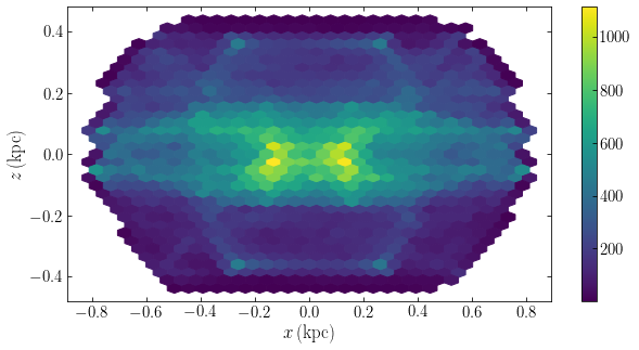
This is starting to look more like a real galaxy, but to fully match the input density profile, we have to build the full orbit library, consisting of such grids as above for each combination of specific energy and specific angular momentum. One simple way to create the specific energy–angular-momentum grid is to first choose a grid of radii and use the energies of circular orbits at those radii as the specific energy grid; at each specific energy, the specific angular momentum can range between minus and positive the specific angular momentum of that circular orbit and the specific angular-momentum grid can thus be made between these two values (note that negative specific angular momentum orbits can be obtain simply by reversing the positive specific angular momentum orbits). We won’t attempt this here, because it would take far too much computational power, but it is a straightforward continuation of what we have implemented so far.
Going through this example, some of the practical issues when running Schwarzschild modeling should start becoming clear. For example, we integrated for a fixed amount of time, but because the radial, vertical, and rotational frequencies of most orbits are incommensurate, it would take infinitely long to actually fully sample the orbit. We therefore have to make a choice and demonstrate that the resulting phase-space distribution function does not change when integrating the orbits for longer. Sampling the orbits is also difficult because of the lack of a full set of integrals of the motion for realistic models of galaxies. Starting from the zero-velocity curve works well for axisymmetric potentials, but for triaxial mass models, the issue more complicated (e.g., van den Bosch et al. 2008). In more complex cases, such as when modeling a barred galaxy, our actual understanding of the types of orbits that occur is still incomplete and properly sampling the orbits is therefore essentially impossible using current methods. Even when we have a way of finding all of the orbits, deciding how to build the grid in this space comes with its own set of difficulties, because we want to build the grid in as natural of a way as possible and avoid sampling the same orbit more than once to reduce the degeneracies in the problem (e.g., Thomas et al. 2004). Because we cannot realistically build a very fine grid, the resulting density distribution is often far from smooth and various techniques exist to alleviate this problem (like “dithering”, running a bunch of orbits near each grid point and averaging their predictions rather than just using a single one). Chaotic orbits can present difficulties as well, e.g., because they can take a very long time to mix if their Lyapunov timescale is large. Because all of the orbits need to be stored, Schwarzschild modeling also exacts heavy memory requirements on the computer system used in the modeling. Made-to-measure modeling (Syer & Tremaine 1996) is an alternative to Schwarzschild modeling where the orbital weights are optimized during orbit integration using a gradient-descent algorithm that overcomes some of these issues (especially that of the memory requirements and of sampling the orbits in complex systems, because it can be initialized using an \(N\)-body simulation). Made-to-measure modeling is equivalent to Schwarzschild modeling in the limit of a large orbit library and short time steps in the orbit integration (Malvido & Sellwood 2015).