
13. Gravitation in elliptical galaxies and dark matter halos
We have so far only considered mass distributions that are either spherical (Chapter 3 and following) or highly flattened into a disk (Chapter 8 and following). However, the mass distributions of two important types of galactic structures fall somewhere in between these two extremes: elliptical galaxies and dark matter halos. Observations of elliptical galaxies show them to be flattened spheroids or ellipsoids and dark matter halos—which we can simulate but not directly observe—are believed to be qualitatively similar to this. The following figure shows an example elliptical galaxy and a simulated Milky-Way-like dark-matter halo:
|
|
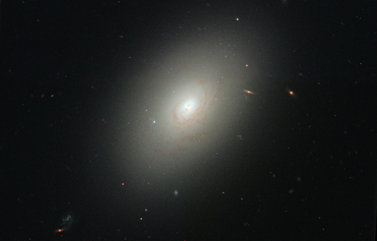
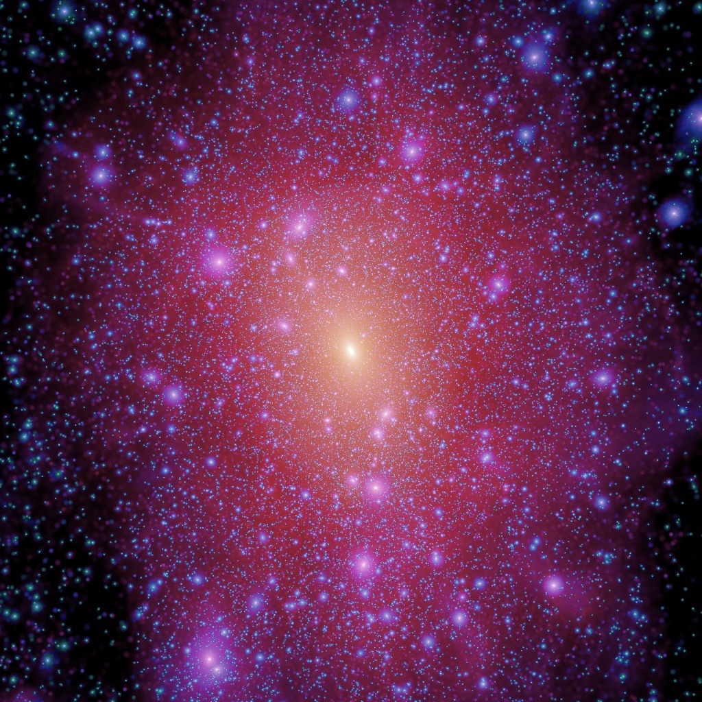
(Credit: left: NASA/ESA Hubble Space telescope; right: Springel et al. 2008a)
The elliptical galaxy NGC 4150 on the let conforms to the expectation for an elliptical galaxy, being a largely featurless blob of light (however, there are some dust lanes indicative of recent star formation). What is of course most striking about the simulated dark-matter halo on the right is the large amount of small-scale structure in the mass distribution (known as subhalos), but most of the mass is in fact contained in a smooth ellipsoidal distribution.
As we will discuss in this chapter, elliptical galaxies and dark-matter halos are either mildly flattened along a single axis, in which case they are axisymmetric with the consequential conservation of the angular momentum along this axis, or along two axes, when they are generally referred to as triaxial. In this part, we discuss how to compute the gravitational potential due to such mass distributions, the properties of orbits in these potentials, and general methods for studying the equilibrium of triaxial models.
13.1. The three-dimensional structure of elliptical galaxies and dark-matter halos
We briefly discussed the radial structure of elliptical galaxies and dark-matter halos in Chapter 2.2.1 and Chapter 3.4.6, but to motivate the somewhat complex methods necessary to study the mass distributions of realistic elliptical galaxies and dark-matter halos, we will start this chapter by taking a closer look at their three-dimensional structure.
The equivalent of Freeman (1970)‘s discovery of the exponential nature of disk galaxies’ radial brightness profile (see Chapter 8.1), is de Vaucouleurs (1948)’s finding that the surface brightness profile of elliptical galaxies drops approximately as \(R^{1/4}\), as shown beautifully for three elliptical galaxies in Figure 21 of de Vaucouleurs (1948)’s paper:
|
|
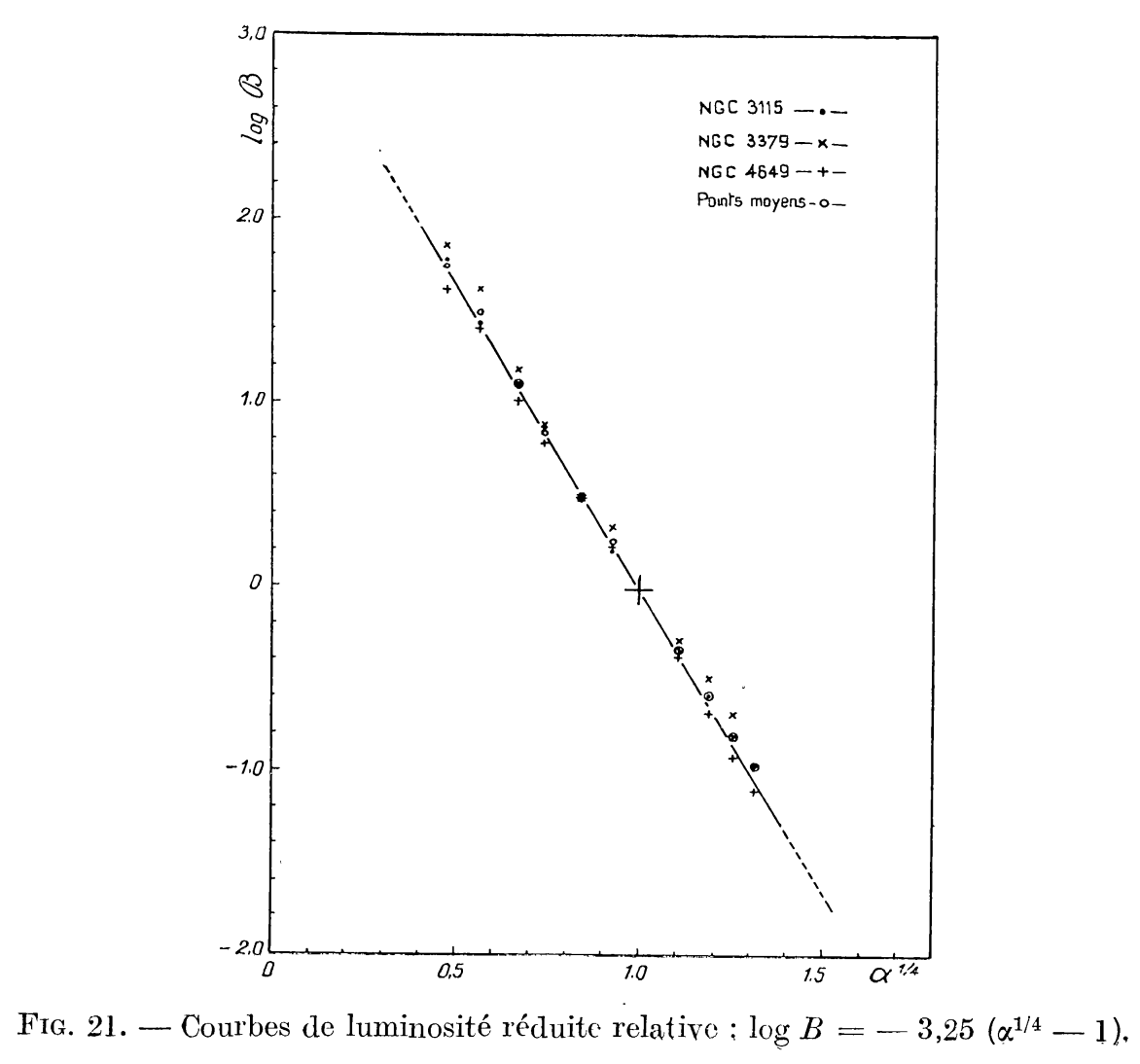
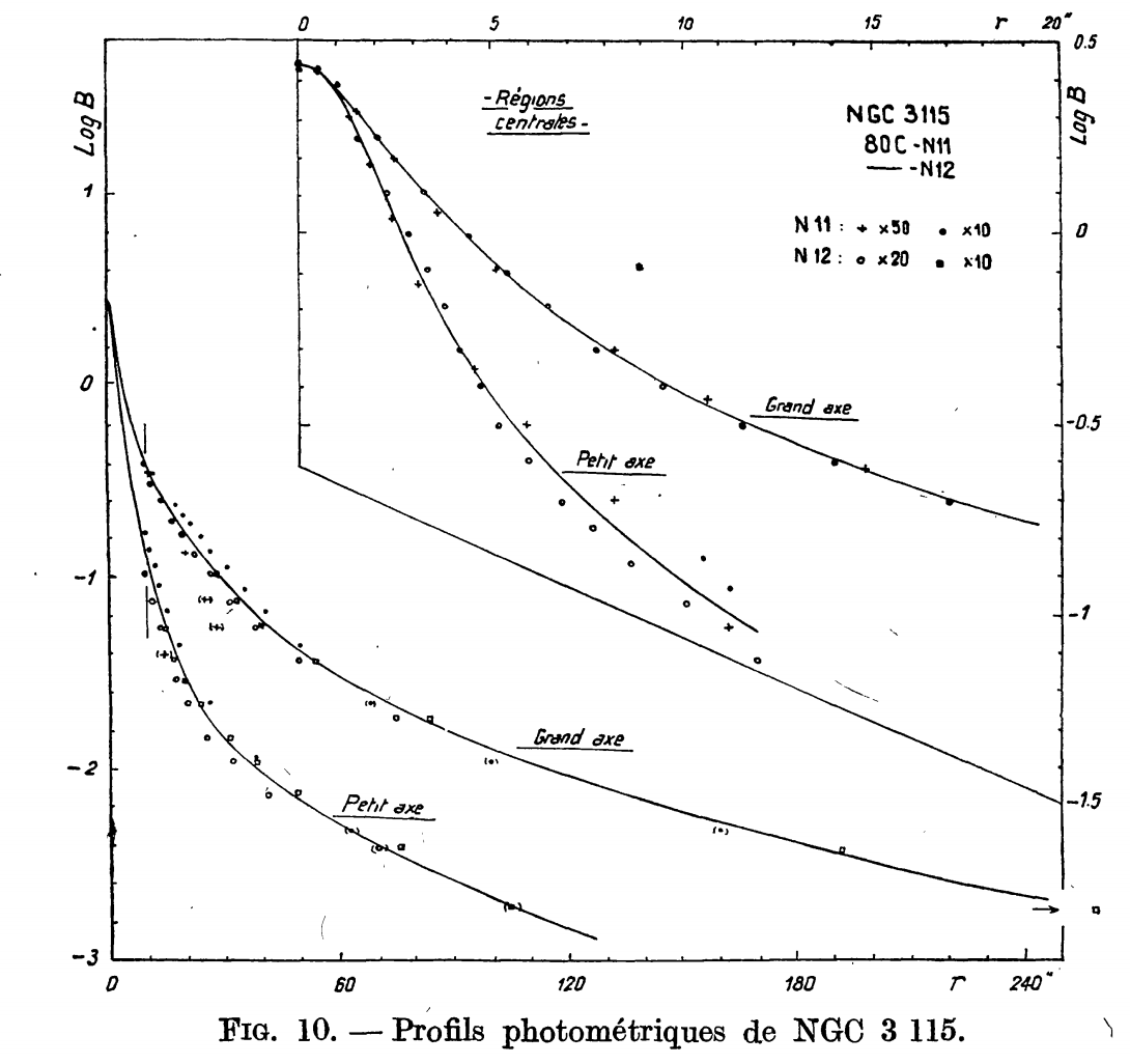
(Credit: de Vaucouleurs 1948: left radial surface brightness profile for three elliptical galaxies (NGC 3115, NGC 3379, and NGC 4549); right: surface brightness profile along the major and minor axis for NGC 3315)
This radial profile, now known as the de Vaucouleurs profile (and even generally referred to as a “law”, even though it’s simply an observation) is given by
where the “3.33” is chosen such that half of the total luminosity is contained with \(R_e\), the effective radius. Thus, the effective radius is equal to the half-light radius, although this is only exactly true if the isophotes are circularly symmetric. It’s often more convenient to express the de Vaucouleurs profile in the form
The de Vaucouleurs profile works well for the larger elliptical galaxies, but for smaller elliptical galaxies, a generalization known as the Sérsic profile is useful (Sersic 1968)
The constant \(b_n\) is again determined such that half of the light is within \(R_e\) and it is approximately given by \(b_n = 2\,n-0.324\) (e.g., \(b_4 = 7.676\) for the de Vaucouleurs profile; Ciotti 1991; see also Ciotti & Bertin 1999 for an improved approximation). Because the Sérsic profile becomes a pure exponential profile for \(n=1\), Sérsic profiles are able to fit photometry of disk and elliptical galaxies and smoothly interpolate between the two.
As discussed in part I, even when a galaxy or dark-matter halo is not spherical, much insight about its structure and dynamics can be gleaned from treating it as such. Because the de Vaucouleurs and Sérsic profiles provide an excellent representation of the observed surface photometry of elliptical galaxies, they are an obvious choice for building a simple spherical model for elliptical galaxies, assuming a constant mass-to-light ratio to turn the surface brightness into a surface mass density. However, the simplicity disappears once one realizes that to build a three-dimensional spherical model, one needs to de-project the two-dimensional surface mass density (e.g., using the Abel integral inversion of Equation 7.16) and, to obtain the gravitational potential and/or field, integrate over the three-dimensional density. While they are straightforward numerically, none of these operations can easily be performed analytically for either the Sérsic profile or its special de Vaucouleurs case (they can all be expressed using the “Fox H function”, a special function so special that it does not appear to be implemented in any programming language!; Baes & Gentile 2011; Baes & van Hese 2011). While precise numerical approximations for the de-projected density and mass profile exist (e.g., Vitral & Mamon 2020), often it is more convenient to approximate the surface density using a form for which the gravitational potential, field, density, and perhaps other properties such as the ergodic distribution function (to, e.g., allow \(N\)-body initialization) is simple.
There are various simple spherical models whose surface brightness approximately follows a de Vaucouleurs profile or, more generally, a Sérsic profile, but some of the most useful are members of the two-power density profiles that we discussed in Chapter 3.4.6. Especially useful in this family are the \(\gamma\) models (Dehnen 1993; Tremaine et al. 1994), because the de-projected de Vaucouleurs density drops approximately as \(r^{-4}\) (at least for \(R \lesssim 8\,R_e\)) as do all \(\gamma\) models. At small radii, the de-projected de Vaucouleurs profile behaves as \(r^{-\gamma}\) with \(1 \lesssim \gamma \lesssim 2\). This range includes the Hernquist profile (\(\gamma = 1\); see Chapter 3.4.6) and the more cuspy Jaffe profile (\(\gamma = 2\)), with the latter being somewhat closer to the de Vaucouleurs profile. These models are useful, because the surface density can be expressed using elementary functions and the ergodic distribution function only contains elementary or common special functions (e.g., Equation 6.80 for the Hernquist profile). An even better approximation is the model with \(\gamma = 3/2\)
where \(M\) is the total mass. For this profile we have that the isotropic velocity dispersion (\(\beta = 0\); see Chapter 6.4.2) and the ergodic and Osipkov-Merritt distribution functions (see Chapter 6.6.1 and 6.6.4.2) can all be expressed using elementary functions and the surface density only involves elliptic integrals (see Appendix B.1.3; Dehnen 1993). Sérsic profiles with \(3 \lesssim n \lesssim 8\) all similarly drop as \(r^{-4}\) out to about ten effective radii and can therefore be well represented by \(\gamma\) profiles, with the \(n=3\) model resembling the Hernquist profile and the \(n = 8\) being close to the Jaffe profile (larger \(n\) implying a stronger cusp). For smaller \(n\), the Sérsic profiles start to drop more precipitously, while the inner profile flattens (Vitral & Mamon 2020).
The de Vaucouleurs profile fits most larger elliptical galaxies well over most of their radial range, but detailed observations of the core regions of ellipticals demonstrates that they deviate from the de Vaucouleurs profile in their central regions. The first detailed observations of the centers of large ellipticals showed that their surface-brightness profiles flatten at small radii and reach a constant value (King 1978). This core region could be well-represented using the King models that we discussed in Chapter 6.6.3, which in this context are known as “isothermal cores”. However, atmospheric blurring affected these observations and because significant blurring causes even a steep central rise to appear as a core, no definite conclusion could be drawn from these early observations (Schweizer 1979). Improved observations culiminating in high-resolution studies with the Hubble Space Telescope soon after its launch cleared up this situation: the cores of elliptical galaxies appear to come in two different classes, with core galaxies showing near-isothermal cores and power-law galaxies a clear power-law behavior (e.g., Kormendy 1985; Crane et al. 1993; Ferrarese et al. 1994; Lauer et al. 1995). The first indication of these two basic types of behavior is shown in this figure from Kormendy (1985)
|
|
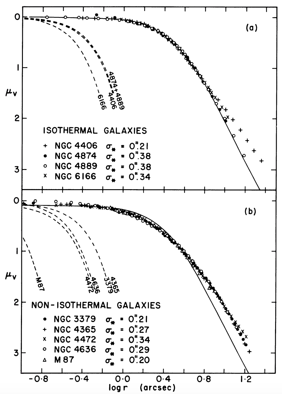
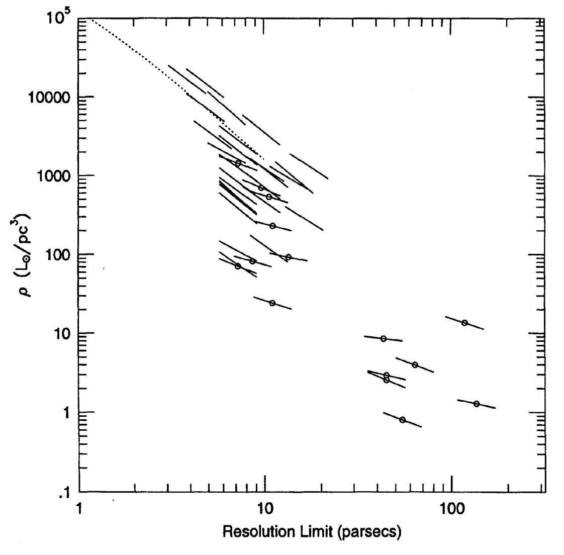
(Credit: left: Kormendy 1985; right: Lauer et al. 1995. The left panel shows surface brightness profiles for the cores of the elliptical galaxies NGC 4406, NGC 4874, NGC 4889, NGC 6166, NGC 3379, NGC 4365, NGC 4636, and M87; these surface brightness profiles fall in two classes: (near-)isothermal cores and non-isothermal (power-law) galaxies. The right panel shows the luminosity density at the innermost resolved point from the comprehensive study of Lauer et al. (1995), which demonstrates that the luminosity density keeps increasing steeply as close as 10 pc from the centers of many elliptical galaxies. Galaxies with near-isothermal cores are marked with a dot in the right panel.)
This figure shows galaxies that are well represented as isothermal cores (King profiles) and galaxies that deviate slightly, but significantly from the isothermal behavior. HST observations showed that even the isothermal galaxies do not reach a constant surface brightness at any resolved radius and keep increasing as close as 10 pc from the center (see the figure from Lauer et al. 1995 above); despite this behavior, the near-isothermal galaxies are referred to as cored galaxies. The near-isothermal galaxies have power-law slopes \(\gamma\) of their surface brightness \(I(R) \propto R^{-\gamma}\) that lie in the range \(0 \lesssim \gamma \lesssim 0.3\), while the power-law galaxies have \(\gamma \approx 1\). Which class an elliptical galaxy falls in correlates with their luminosity: more luminous ellipticals are near-isothermal (core) galaxies, while less luminous ellipticals display a \(\gamma \approx 1\) power-law (Kormendy 1985). The power-law behavior discussed here is that of the surface brightness, which is a projection of the 3D luminosity density. We can de-project it using the Abel inversion of Equation (7.16), which can be difficult. Roughly speaking, near-isothermal galaxies have inner luminosity density slopes \(\alpha\) in \(L(r) \propto r^{-\alpha}\) that are \(0 \lesssim \alpha \lesssim 1\) and thus shallow cusps, while the power-law galaxies with \(\gamma \approx 1\) have steeper cusps with \(1 \lesssim \alpha \lesssim 2\). To represent the surface-brightness profiles of the centers of ellipticals, an often-used form is the so-called “Nuker profile” (Lauer et al. 1995; Byun et al. 1996; named after the team that proposed it)
This profile is such that at \(R \ll R_b\) the surface brightness is approximately \(I(R) \propto R^{-\gamma}\), while at \(R \gg R_b\), approximately \(I(R) \propto R^{-\beta}\); the parameter \(\alpha\) sets how sharply the profile transitions between these two behaviors at \(R \approx R_b\). This profile is similar to the two-power density profiles of Chapter 3.4.6, but note that the Nuker profile is for the surface-brightness. To obtain the three-dimensional density, one has to de-project the Nuker profile using the Abel inversion of Equation (7.16). This, however, cannot be done using elementary or simple special functions (again, instead, requiring the dreaded “Fox H function” ; Baes 2020) and using the Nuker profile for dynamical studies is therefore difficult. Approximating the surface-brightness with a suitable two-power density profile of Chapter 3.4.6 is therefore again a useful strategy for dynamical studies of the inner regions of elliptical galaxies.
The isophotes of elliptical galaxies are, as their name implies, generally elliptical. Contours of the projected shape of elliptical galaxies are typically well-represented as a set of eccentric ellipses with axis ratio \(b/a\) and ellipticity \(\varepsilon = 1-b/a\). For example, in the Hubble classfication scheme (Hubble 1926), elliptical galaxies are arranged by ellipticity starting from \(\varepsilon=0\) to \(\varepsilon = 0.7\), which is about as elliptical as any observed elliptical galaxy ever gets; the Hubble classification explicitly uses this projected ellipticity as part of its name, as \(\mathrm{E}[10\varepsilon]\), where \([\cdot]\) rounds to the nearest integer (e.g., E2 indicates a galaxy with ellipticity 0.2). Some examples are shown in Hubble (1926)’s original paper:
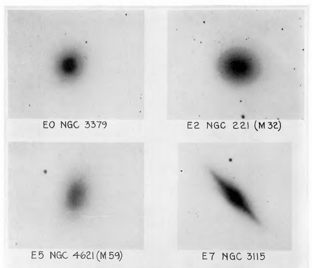
(Credit: adapted from Hubble 1926; see Figure 10 from de Vaucouleurs 1948 for more detailed photometry along the major and minor axis for NGC 3115)
For any external elliptical galaxy, we can only measure its projected shape on the sky and it is therefore not immediately clear that elliptical galaxies cannot be represented as axisymmetric distributions seen from a random viewpoint. The simplest interpretation of the projected elliptical shape was therefore that the intrinsic shape of elliptical galaxies was axisymmetric with an intrinsic axis ratio \(q\) that satisfies \(q < 1-\varepsilon\). Axisymmetric models were therefore the starting point for interpreting observations of elliptical galaxies (e.g., Wilson 1975). However, various lines of evidence argue against axisymmetric models for elliptical galaxies. Photometrically, the distribution of observed shapes is inconsistent with that resulting from projecting an intrinsically axisymmetric distribution with a range of axis ratios (Ryden 1996). Additionally, the projected major axis of many elliptical galaxies twists on the sky (known as isophotal twists; King 1978), which could be due to an actual twist of the major axis of axisymmetric shells or, more naturally, result from a smooth change in the axis ratios of a triaxial model (Binney 1978a); in both cases, the overall mass distribution is non-axisymmetric. Kinematically, flattened axisymmetric models are expected to rotate significantly (Binney 1978b; see Chapter 15.2), while early observations indicated only mild rotation in many ellipticals (Bertola & Capaccioli 1975; Illingworth 1977). Triaxial bodies typically contain stable orbits that circulate around the major axis (in addition to orbits that circulate around the minor axis, which also exist in axisymmetric mass distributions), which gives rise to observed rotation along the projected minor-axis (Contopoulos 1956; Binney 1985); small amounts of such minor-axis rotation have been observed (Franx et al. 1991). All of these observations indicate that there is at least some triaxiality in the mass distributions of elliptical galaxies. Modern observational campaigns that measure two-dimensional kinematics of many elliptical galaxies separate ellipticals into two classes based on their mean rotation: slow rotators and fast rotators (e.g., Cappellari 2016). The lower-mass fast rotators have kinematics that aligns with their observed photometry; this lack of minor-axis rotation indicates that they are close to axisymmetric and their orbital structure is therefore not so different from that of disks. Slow rotators, which are typically more massive, are likely mildly triaxial (e.g., Weijmans et al. 2014).
One final aspect of the shape of elliptical galaxies that is important is that their isophotes systematically deviate from being pure ellipses in a manner that is correlated with other galaxy properties. Deviations from pure elliptical isophotes are typically measured by first finding the best-fit pure ellipse for a given isophote and then expanding the radial differences \(\Delta r\) between the observed isophote and the ellipse model as a function of azimuthal angle \(\theta\), in coordinates where the ellipse’s major axis is at \(y=0\), as (e.g., Bender & Moellenhoff 1987)
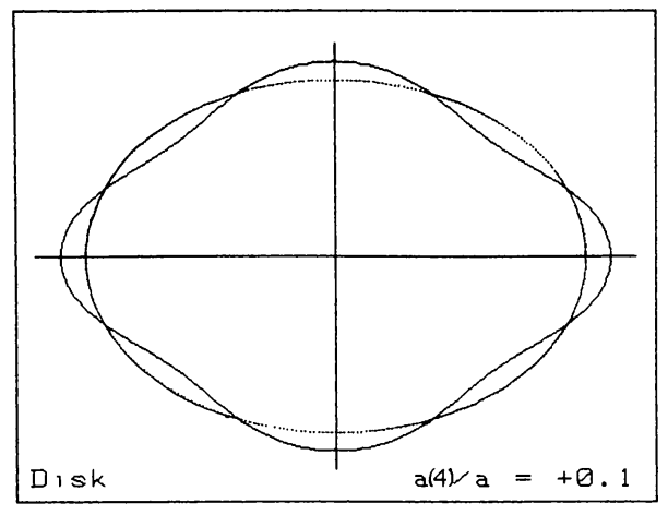
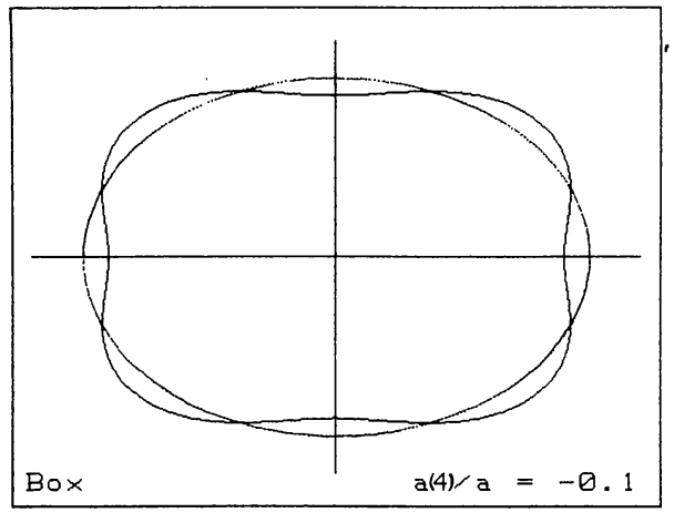
Because the deviations are measured with respect to the best-fitting ellipse, the coefficients \(a_0\), \(a_1\), \(b_1\), \(a_2\), and \(b_2\) are all \(\approx 0\) and the higher-order coefficients then measure deviations from ellipticity. Among the coefficients with \(n \leq 5\), the \(a_4\) cofficient is the only one that describes deviations that are symmetric with respect to both the major and minor axis of the ellipse, which is generally what is observed. Therefore, the \(a_4\) coefficient is typically the only non-zero \(n\leq5\) coefficient. Its importance is that it describes deviations from ellipticity that are either disky, for \(a_4 > 0\), or boxy, for \(a_4 < 0\). The strength of the diskyness or boxyness is determined by the ratio \(a_4/a\) of the \(a_4\) coefficient to the semi-major axis of the ellipse \(a\). The following figure displays two archetypical examples from the original disky-vs-boxy analysis of Bender et al. (1988) as well as an exaggerated illustration of the effect of disky or boxy \(a_4\) coefficients on an isophote’s shape:
|
|
|
|
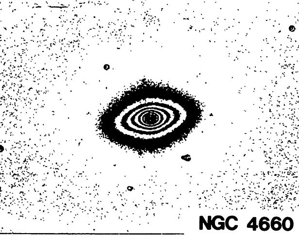
(Credit: Bender et al. 1988)
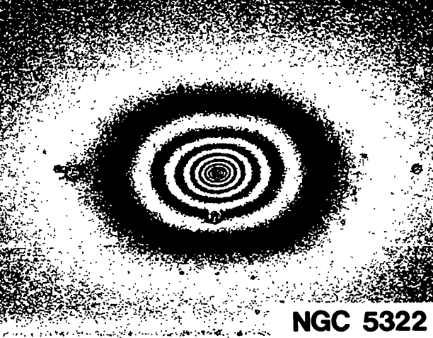
We see that even a small disky \(a_4\) coefficient (\(a_4/a \approx 0.03\) for NGC 4660) makes a galaxy’s isophotes resemble those of a disk galaxy (see, for example, the isophotes of NGC 4244 in Chapter 8.1). A small boxy \(a_4\) coefficient (\(a_4/a\approx -0.01\) for NGC 5322) makes a galaxy almost look like a rectangle with rounded corners. The importance of disky vs. boxy isophotes is that this property is correlated with other galaxy properties and, in particular, the slow rotators discussed above generally have boxy isophotes, while the fast rotators have disky isophotes. We will discuss the relations between the different observational properties of elliptical galaxies discussed in this section in more detail in Chapter 17, in particular in Section 17.4.
The second class of mass distributions that we study in this part are dark-matter halos. Observational constraints of the shape of dark-matter halos are scant, but they have been studied in detail in numerical simulations. Dissipationless simulations—also known as dark-matter only simulations—create galactic dark-matter halos that are strongly triaxial and highly flattened (e.g., Frenk et al. 1988; Dubinski & Carlberg 1991; Jing & Suto 2002). Moreover, compared to elliptical galaxies, dark matter halos are much more flattened. Labeling the relative lengths of the major, intermediate, and minor axis as \(a > b > c\), dissipationless dark-matter halos have typical values of \(b/a \approx 0.7\) and \(c/a \approx 0.5\). Some of these results are illustrated in the following figures:
|
|
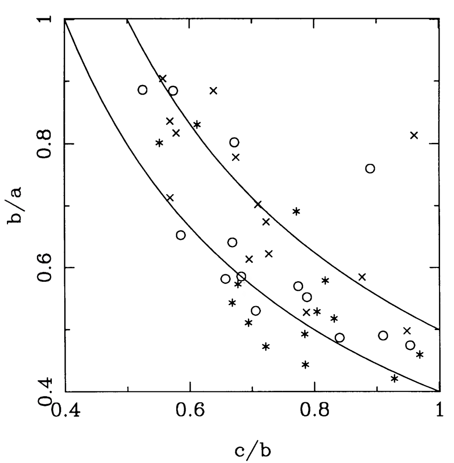
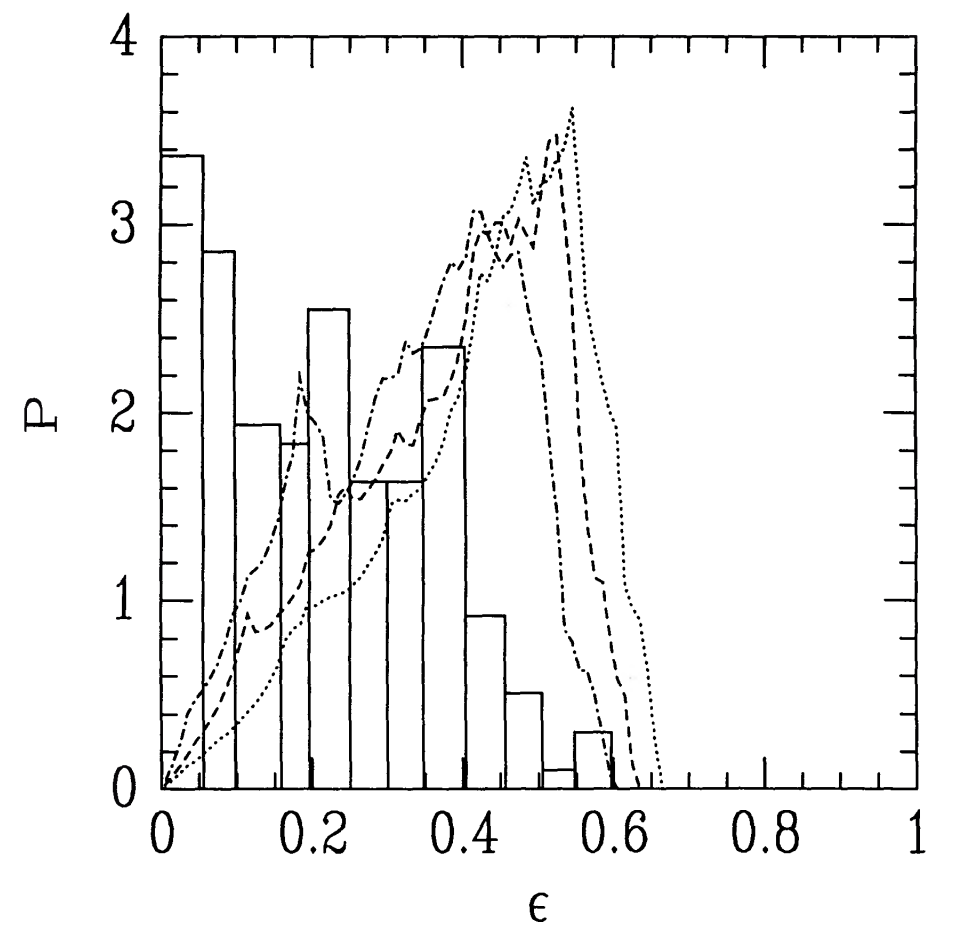
(Credit: Dubinski & Carlberg 1991; left panel shows axis ratios of simulated dark matter halos at different radii (25 kpc [asterisks], 50 kpc [circles], and 100 kpc [crosses]); right panel displays the distribution of observed ellipticities in the sample of elliptical galaxies of Binney & de Vaucouleurs 1981 compared the projected ellipticities of simulated dark matter halos).
The shape of a triaxial density is also often summarized using the triaxiality parameter \(T\) defined as
From the definition of \(T\), it is clear that oblate (\(a = b > c\)) and prolate (\(a > b = c\)) distributions have \(T=0\) and \(T=1\), respectively. Mass distributions with \(T = 0.5\) are then maximally-triaxial. For the canonical \(b/a \approx 0.7\), \(c/a \approx 0.5\) mentioned above, we get \(T \approx 0.7\). Generally, dissipationless dark-matter halos are more prolate than oblate (\(T > 0.5\)). The shape parameters \(b/a\), \(c/a\), and \(T\) depend on radius, with a generally more axisymmetric, prolate shape within a tenth of a virial radius (\(T \approx 1\)) deforming to a strongly triaxial shape near the virial radius (\(T \approx 0.5\); e.g., Chua et al. 2019). We discuss the effect of the central galaxy on the shape of the dark matter in Chapter 14.4.3.
Numerical studies of the orbital structure of such triaxial distributions show that they are stable over the age of the Universe (e.g., Aarseth & Binney 1978; Schwarzschild 1979; van Albada 1982). The dissipational growth of a baryonic component in galaxies has the effect of making the inner parts of dark-matter halos axisymmetric (e.g., Dubinski 1994), but the outer regions of halos remain triaxial. Aside from affecting the dynamics of stars, clusters, satellites, and everything else embedded within the dark matter halos that host galaxies, the shape of dark matter halos also holds valuable clues about the nature of dark matter, because, for example, strong self-interactions between dark matter particles would tend to sphericalize it (e.g., Spergel & Steinhardt 2000).
Therefore, to fully understand the structure of elliptical galaxies and dark matter halos, we need to investigate the gravitational potential, orbits, and equilibrium states of triaxial mass distributions. We will start by discussing simple models for flattened-axisymmetric and triaxial distributions, which have shapes and orientations that are constant with radius. However, it is clear from the discussion above that realistic galaxies and dark-matter halos have shapes that change with radius: Elliptical galaxies with isophote twists either require the orientation or the shape to change with radius (and perhaps both!); dark-matter halos are likely axisymmetric and only mildly flattened in their inner parts due to the growth of the baryonic component, while they are expected to be strongly triaxial in their outer parts. To handle this complexity, we will present several general, yet practical, approaches to solving the Poisson equation for any mass distribution.
13.2. Gravitational potentials for mildly-flattened and triaxial mass distributions
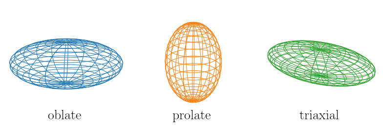
Calculating the gravitational potential for a general, triaxial mass distribution is a difficult problem. In this section, we first tackle the simpler problem of how to compute the potential for an oblate spheroidal (axisymmetric) shell and generalize it to a mass distribution where the density is constant on oblate spheroids—the shape obtained when rotating an ellipse around its major or minor axis. We then discuss the more general case where the density is constant on (triaxial) ellipsoids. The three qualitatively different geometries that we consider are shown in the following figure. They are (a) oblate or flattened spheroids, (b) prolate or elongated spheroids, and (c) triaxial ellipsoids:
[13]:
from mpl_toolkits.mplot3d import Axes3D
# we fiddle with the aspect ratio here
# to make the axes line up more tightly
# (adjusted for at the bottom)
stretch= 1.5
fig= figure(figsize=(11,11))
coeffs_sets = [(1.,1.,0.5),
               (1.,1.,2.),
               (1.,2.,.75)]# Coefficients in (x/a)**2 + (y/b)**2 + (z/c)**2 = 1
labels= ['oblate','prolate','triaxial']
# Spherical angle grid for parametric ellipsoids
phi= numpy.linspace(0.,2.*numpy.pi,101)
theta= numpy.linspace(0.,numpy.pi,101)
for ii,coeffs in enumerate(coeffs_sets):
    ax= fig.add_subplot(1,3,ii+1,projection='3d')
    # Radii in x,y,z
    rx, ry, rz= coeffs
    # Convert to cartesian coordinates
    x= rx*numpy.outer(numpy.cos(phi),numpy.sin(theta))
    y= ry*numpy.outer(numpy.sin(phi),numpy.sin(theta))
    z= rz*numpy.outer(numpy.ones_like(phi),numpy.cos(theta))
    # Plot as wireframe
    ax.plot_wireframe(x, y, z,rstride=5,cstride=6,lw=1.,
                      color=rcParams['axes.prop_cycle'].by_key()['color'][ii])
    maxr= max(rx,ry,rz)
    for axis in 'xy':
        getattr(ax,'set_{}lim'.format(axis))((-maxr/stretch,maxr/stretch))
    getattr(ax,'set_zlim'.format(axis))((-maxr/stretch,maxr/stretch))
    ax.view_init(15+ii*10,20.)
    ax._axis3don = False
    annotate(r'$\mathrm{{{label}}}$'.format(label=labels[ii]),
             (0.5,0.05),xycoords='axes fraction',
             horizontalalignment='center',size=28.)
tight_layout();
13.2.1. The potential of a spheroidal shell
We start by computing the gravitational potential of mass distributions that are axisymmetric and constant on ellipses in the \((R,z)\) plane that all have the same center and the same axis ratio. The density is then a function only of the quantity \(m\) that is related to \((R,z)\) as
with \(q > 0\). When \(q < 1\), this is the equation of an ellipse with its major axis along \(z=0\) and with eccentricity \(e = \sqrt{1-q^2}\); the three-dimensional surface corresponding to this is an oblate spheroid. When \(q > 1\) we get a prolate spheroid instead, with Equation \(\eqref{eq-oblate-prolate-mq}\) the equation of an ellipse with its major axis along \(R=0\) and eccentricity \(e = \sqrt{1-1/q^2}\).
Oblate and prolate spheroids require a similar, but different treatment, and we start by computing the gravitational potential of a thin oblate shell of matter with total mass \(M_\mathrm{shell}\) and \(\rho \propto \delta(m-m_0)\) with \(m_0\) the location of the shell and where \(m\) and \(m_0\) are computed with the same, constant \(q < 1\). Because the Laplace equation \(\nabla^2 \Phi =0\) can be solved using the separation-of-variables technique in oblate spheroidal coordinates (see below) in which, for the correct definition of the coordinate system, we can also express the density as being a function of only a single coordinate, we switch to this coordinate system. Oblate spheroidal coordinates are defined by a focal length \(\Delta\) and form a transformation of the \((R,z)\) coordinates of the cylindrical coordinate system (the azimuthal angle \(\phi\) is unchanged)
where \(u \geq 0\) and \(0 \leq v \leq \pi\) and \(\Delta\) is the constant focal length. For completeness, the full transformation between oblate spheroidal and cartesian coordinates is given by
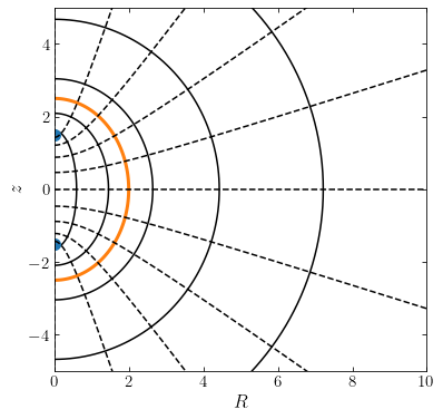
In the \((R,z)\) plane, curves of constant \(u\) are (half-) ellipses centered on the origin with focus at \((R,z) = (\Delta,0)\) and eccentricity \(1/\cosh u\), while curves of constant \(v\) are hyperbolae which are the normals to the ellipses. This is illustrated in the following figure, which displays curves of constant \(u\) as solid lines and curves of constant \(v\) as dashed lines, with the focus \((\Delta,0)\) shown as a large dot:
[16]:
figsize(6,6)
from galpy.util import coords
delta= 1.5 # Focal length
# First plot curves of constant u
us= numpy.linspace(0.3,1.75,5)
vs= numpy.linspace(0.,numpy.pi,101)
for tu in us:
    Rs,zs= coords.uv_to_Rz(tu*numpy.ones_like(vs),vs,
                           delta=delta,oblate=True)
    plot(Rs,zs,'k-')
# Plot the focus
plot([delta],[0.],'o',ms=10.)
# Also plot a shell with m_0 = 2
m0= 2.
u0,v0= coords.Rz_to_uv(m0,0.,delta=delta,oblate=True)
Rs,zs= coords.uv_to_Rz(u0*numpy.ones_like(vs),vs,
                       delta=delta,oblate=True)
plot(Rs,zs,'-',lw=3.)
# Then plot curves of constant v
us= numpy.linspace(0.,10.,101)
vs= numpy.linspace(0.,numpy.pi,11)
for tv in vs:
    Rs,zs= coords.uv_to_Rz(us,tv*numpy.ones_like(us),
                           delta=delta,oblate=True)
    plot(Rs,zs,'k--')
xlim(0.,5.)
ylim(-2.5,2.5)
xlabel(r'$R$')
ylabel(r'$z$');
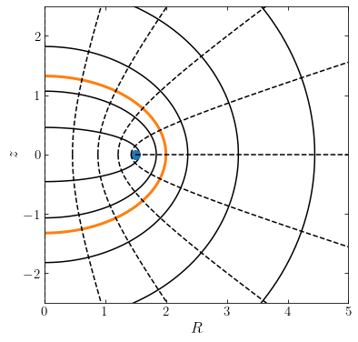
A shell with \(m = m_0\) corresponds to a shell with constant \(u = u_0\) if we set
The coordinate \(u_0\) of the shell can be found from \(\tanh u_0 = q\) or from \(\cosh u_0 = m_0/\Delta = 1/e\). As an example, the thick shell highlighted in the above figure has \(m_0 = 2\) and \(q \approx 0.66\) with \(\Delta = 1.5\).
Thus, in the oblate spheroidal coordinate system with focus set by Equation \(\eqref{eq-oblate-shell-focus}\), the shell with constant density \(\rho(m) \propto \delta(m-m_0)\) and axis ratio \(q\) corresponds to a density \(\rho(u,\phi,v) \propto \delta(u-u_0)\). Inside and outside of the shell with \(m=m_0\), the Poisson equation becomes the Laplace equation \(\nabla^2 \Phi = 0\) and we can solve for the potential of the shell by solving the Laplace equation inside and outside of the shell and connect the two solutions at the location of the shell. As already mentioned above, oblate spheroidal coordinates is one of a small number of coordinate systems for which the Laplace equation can be solved using the method of separation of variables. In this method, solutions to the Laplace equation of the form \(\Phi_{mn}(u,\phi,v) = U_{mn}(u)\,\Pi_n(\phi)\,V_{mn}(v)\) can be found, the functions \(U_{mn}\), \(\Pi_n\), and \(V_{mn}\) are orthogonal (when integrating over the full volume) and form a basis for all smooth functions, and general solutions can be expressed as the sum over the basis functions \(\Phi_{mn}(u,\phi,v)\). A direct consequence of this is that if the density of the thin shell that forms the boundary condition for solving the Laplace equation is only a function of a single coordinate, in this case \(u\), then the solution of the Laplace equation can only depend on the same coordinate. Thus, the potential \(\Phi\) corresponding to the shell with \(\rho(u,\phi,v) \propto \delta(u-u_0)\) can only be a function of \(u\): \(\Phi \equiv \Phi(u)\).
Before working out what the potential \(\Phi(u)\) of the shell is, we can determine the behavior of the potential at \(r \gg m_0\) simply by considering the properties of the oblate spheroidal coordinate system. As we have discussed above, contours of constant \(u\) in the \((R,z)\) plane are ellipses with the focus at \((R,z) = (\Delta,0)\) and axis ratio \(\tanh u\). As is clear from the above figure and from the behavior of the hyperbolic tangent function at large values of its argument (\(\tanh u \rightarrow 1\) as \(u \rightarrow \infty\); e.g., \(\tanh(2.65) = 0.99\)), these ellipses becomes more and more circular as \(u\) increases. This implies that the potential far from the shell becomes spherical: no matter how flattened the oblate shell is, at large distances from it the shell gives rise to a spherical gravitational potential. Because the shell has a finite mass \(M_\mathrm{shell}\), the radial behavior of the potential approaches that of a point-mass potential, \(\Phi(r) = -GM/r\) at large \(r\). Thus, without doing any calculation, we have determined the asymptotic behavior of the potential of an oblate shell.
To work out the Laplace equation and the gravitational field in the oblate spheroidal coordinate system, we need the expressions for the gradient \(\nabla\) and Laplacian \(\nabla^2\) in this coordinate system. The gradient is given by
and the Laplacian is given by
Because the potential only depends on \(u\) for a shell with constant density in \((\phi,v)\), the Laplace equation for the potential outside of the shell luckily simplifies significantly, because we only need to keep derivatives with respect to \(u\). After dropping an unnecessary pre-factor, we are left with
The general solution to this equation is
Therefore, the potential of the shell at \(u < u_0\) is given by
while that outside of the shell is
This general solution has four constants \((A_\mathrm{in},B_\mathrm{in},A_\mathrm{out},B_\mathrm{out})\) that we need to determine from boundary conditions at \(u=\infty\), \(u=0\), and \(u=u_0\). We set \(B_\mathrm{out}\) such that \(\lim_{u\rightarrow\infty} \Phi(u) = 0\); because \(\sin^{-1}(1/\cosh u)\) goes to zero as \(u\rightarrow\infty\), this means that we set \(B_\mathrm{out} = 0\). The \(u\) component of the gravitational field is given by
At the center of the shell, \((u,v) = (0,0)\), this field is equal to \(-A_\mathrm{in}/\Delta\). However, from symmetry we know that the field at the center of the shell must vanish and therefore \(A_\mathrm{in} = 0\). Continuity of the potential at \(u=u_0\) then leaves us with the following potential with a single free parameter
Similar to how we determined a relation between the surface density and the gradient of the potential for a razor-thin disk in Chapter 8.2.1 by integrating the Poisson equation over a small volume around the disk and using the divergence theorem, we can integrate the Poisson equation over a volume that encompasses the entire shell in \((\phi,v)\) in a small range of \(u\) around \(u_0\). To do this integration, we need the surface element in \((\phi,v)\) which is \(\Delta^2\,\cosh u\,\sin v\,\sqrt{\sinh^2u+\cos^2v}\)). This leads to a relation between the surface integral over the gradient given in Equation \(\eqref{eq-oblate-shell-force}\) and the total mass
or
which gives the following relation between \(A\) and \(M_\mathrm{shell}\)
The gravitational potential of an oblate shell of mass \(M_\mathrm{shell}\) is therefore
As \(u \rightarrow \infty\), the transformations in Equations \(\eqref{eq-oblate-coords-1}\) and \(\eqref{eq-oblate-coords-2}\) approach
because \(\tanh u \rightarrow 1\). The oblate coordinate system approaches the spherical coordinate system, with \(u\) a different representation of the radial coordinate \(r\): \(\Delta \cosh u = r\). Because \(\sin^{-1}(1/\cosh u) \rightarrow 1/\cosh u\) when \(u \rightarrow \infty\), the potential then approaches \(\Phi(u) \rightarrow -GM_\mathrm{shell}/\Delta/\cosh u =-GM_\mathrm{shell}/r\), the point-mass potential.
The following figure shows the potential \(\Phi(u)\) for the shell highlighted in the figure above as a function of \(u\). This potential is compared to the potential along \(z=0\) for a spherical shell with radius \(r_0 = m_0\) and one with radius \(r_0 = q\,m_0\) (which are the spherical shells that touch the spheroical shell on the inside and outside):
[15]:
figsize(7,5)
xs= numpy.linspace(0.,10.,1001)
delta= 1.5
m0= 2.
u0,v0= coords.Rz_to_uv(m0,0.,delta=delta,oblate=True)
q= numpy.tanh(u0)
us= numpy.linspace(0.,u0,101)
line_oblate= plot(us,
                  -1/delta*numpy.arcsin(1./numpy.cosh(u0*numpy.ones_like(us))),
                 label=r'$\mathrm{Oblate\ shell}$',zorder=2)
us= numpy.linspace(u0,5.,101)
plot(us,-1/delta*numpy.arcsin(1./numpy.cosh(us)),
     color=line_oblate[0].get_color())
# If spherical with r_0 = m_0
us= numpy.linspace(0.,u0,101)
line_sphere= plot(us,-1./delta/numpy.cosh(u0)*numpy.ones_like(us),zorder=1,
                 label=r'$\mathrm{Spherical\ shell\ with}\ r_0 = m_0$')
us= numpy.linspace(u0,5.,101)
plot(us,-1./delta/numpy.cosh(us),color=line_sphere[0].get_color())
# If spherical with r_0 = m_0*q
us= numpy.linspace(0.,u0,101)
line_sphere2= plot(us,-1./q/delta/numpy.cosh(u0)*numpy.ones_like(us),
                   zorder=0,
                   label=r'$\mathrm{Spherical\ shell\ with}\ r_0 = q\,m_0$')
us= numpy.linspace(u0,5.,101)
plot(us,-1./delta/q/numpy.cosh(us),color=line_sphere2[0].get_color())
ylim(-1.,0.05)
xlabel(r'$u$')
ylabel(r'$\Phi(u)$')
legend(handles=[line_oblate[0],line_sphere[0],line_sphere2[0]],
       fontsize=18.,loc='lower right',frameon=False);
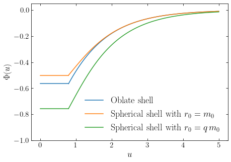
The oblate shell creates a potential well that is somewhere between that of the enclosing spherical shells with the same mass: shallower than the inscribed spherical shell, but deeper than that of the spherical shell that is outside of the spheroidal shell. At \(u \gg u_0\) all of the potential converge to the same \(1/r\) behavior.
The potential of a prolate shell of matter (Equation \(\eqref{eq-oblate-prolate-mq}\) with \(q>1\)) can be obtained using a similar procedure as that we followed for an oblate shell, but working instead in prolate spheroidal coordinates, which are defined in a similar manner to the oblate spheroidal coordinates in Equations \(\eqref{eq-prolate-coords-1}\) and \(\eqref{eq-prolate-coords-2}\)
In the \((R,z)\) plane, curves of constant \(u\) are again (half-) ellipses centered on the origin, but they now have two foci \((R,z) = (0,\pm\Delta)\) and their major axis lies along \(R=0\); curves of constant \(v\) are again hyperbolae which are the normals to the ellipses. This is again illustrated in the following figure, which displays contours of constant \(u\) and \(v\) in the same way as in the figure above for oblate spheroidal coordinates
[17]:
figsize(6,6)
from galpy.util import coords
delta= 1.5 # Focal length
# First plot curves of constant u
us= numpy.linspace(0.3,1.75,5)*1.3
vs= numpy.linspace(0.,numpy.pi,101)
for tu in us:
    Rs,zs= coords.uv_to_Rz(tu*numpy.ones_like(vs),vs,
                           delta=delta)
    plot(Rs,zs,'k-')
# Plot the foci
plot([0.,0.],[delta,-delta],'o',ms=10.)
# Also plot a shell with m_0 = 2
m0= 2.
u0,v0= coords.Rz_to_uv(m0,0.,delta=delta)
Rs,zs= coords.uv_to_Rz(u0*numpy.ones_like(vs),vs,
                       delta=delta)
plot(Rs,zs,'-',lw=3.)
# Then plot curves of constant v
us= numpy.linspace(0.,10.,101)
vs= numpy.linspace(0.,numpy.pi,11)
for tv in vs:
    Rs,zs= coords.uv_to_Rz(us,tv*numpy.ones_like(us),
                           delta=delta)
    plot(Rs,zs,'k--')
xlim(0.,10.)
ylim(-5.,5.)
xlabel(r'$R$')
ylabel(r'$z$');
Similar to the oblate shell, a prolate shell’s gravitational potential is constant inside of the shell. We do not derive the full expression for the potential of a prolate shell here.
13.2.2. Potentials of ellipsoidal systems
Just like we derived Equation (3.28) for the potential for any spherical density distribution by splitting the density into shells and adding the contribution from all of these shells, we can derive the potential for an spheroidal density distribution that is constant on similar ellipsoids (ellipses with the same axis ratio \(q\)) such that the density is a function of \(m\): \(\rho \equiv \rho(m)\). We will work this out for an oblate spheroid before generalizing to the general triaxial case. This is not quite as simple as it was for spherical densities, because the foci of each of these similar ellipsoids differ and this needs to be taken into account. The first order of business is to split the density \(\rho(m)\) into a set of infinitesimal spheroids with mass \(\mathrm{d}M(m)\), such that we can obtain the potential by summing over the potentials of all these thin shells. The volume of an oblate spheroid with major axis \(m\) and flattening \(q\) is \(V = 4\pi\,m^3\,q/3\)—which reduces to the volume of a sphere for \(q=1\)—so the amount of mass \(\mathrm{d}M(m)\) that lies between the shells with coordinates \(m\) and \(m+\mathrm{d}m\) is
because \(\mathrm{d}m\) is infinitesimal. We then have to add the potential from a sequence of thin shells with masses \(\mathrm{d}M(m)\) and we first re-write the potential of a thin shell from Equation \eqref{eq-triaxialgrav-potoblateshell} to be a function of its semi-major axis \(m\) as much as possible. For a shell with mass \(\mathrm{d} M(m)\) we have that
To obtain the potential at a point \((R,z)\) that corresponds to the shell indexed by \(\tilde{m} = \sqrt{R^2+z^2/q^2}\), we sum over the contributions to the potential interior and exterior to this shell. The contribution from shells exterior to the shell with \(m = \tilde{m}\) is from Equations \eqref{eq-triaxialgrav-dM} and \eqref{eq-triaxialgrav-potoblateshell2}
As will become clear below, it is convenient to write this in terms of the function \(\psi(m)\) defined as
for which \(\Phi_{\mathrm{ext}}\) becomes
Similarly, the contribution from shells interior to the shell with \(m=\tilde m\) is
In this equation, \(u\) is a function of \(m\), \(R\), and \(z\) through the requirement that \(u\) is the coordinate of \((R,z)\) in the oblate coordinate frame defined using \(\Delta = m e\) (and which is therefore different for each \(m\) in the integral). From Equations \eqref{eq-oblate-coords-1} and \eqref{eq-oblate-coords-2}, it is clear that
To get rid of the inverse sine function in Equation \eqref{eq-triaxialgrav-phiint-1}, we can integrate by parts and use the properties of hyperbolic functions to obtain
From Equation \eqref{eq-triaxialgrav-umRz}, it is clear that \(m=0\) requires \(1/\cosh u = 0\) and \(\sinh u = \infty\), while \(m=\tilde{m}\) has \(1/\cosh u = e\) and \(\sinh u = q/e = \sqrt{1-e^2}/e\), such that we can simplify the first term and properly write the integration limits as
where \(m\) in the integral is implicitly defined by Equation \eqref{eq-triaxialgrav-umRz} written solely in terms of \(\sinh u\) as
Adding up the contribution from shells exterior to \((R,z)\) from Equation \eqref{eq-triaxialgrav-phiext} and that from shells interior from Equation \eqref{eq-triaxialgrav-phiint-3}, we therefore get the potential
Standard practice is to re-write the integral further by defining a new integration variable \(\tau\) defined as
where \(a_0\) is an arbitrary constant. Then \(\tau\) is a function of \((m,R,z)\) by the transformed Equation \eqref{eq-triaxialgrav-umRz-2}
and the potential becomes
As \((R,z) \rightarrow \infty\), this potential approaches zero (because \(\int_0^\infty\mathrm{d}\tau \big/\left[(\tau+a_0^2)\,\sqrt{\tau+q^2\,a_0^2}\right] = 2\,\sin^{-1} e / e\)).
The right-hand side of Equation \eqref{eq-triaxialgrav-pot-oblate} is a function of \((R,z)\) through Equation \eqref{eq-triaxialgrav-mtau-Rz-oblate}. The \(\psi(m)\) function in Equation \(\eqref{eq-psi-triaxial}\) can be computed analytically for many density profiles of interest and the potential can then be obtained efficiently using a one-dimensional quadrature. Moreover, expressions for the gravitational field, which we will give below after generalizing this result to triaxial ellipsoids, only involve the derivative of \(\psi(m)\), which is simply proportional to the density and the gravitational field can thus be computed using a one-dimensional quadrature for any spheroidal mass distribution.
Ellipsoidal systems are the triaxial generalization of the oblate and prolate spheroids that we have considered above. They have densities that are constant on similar ellipsoids defined by
The systems of oblate and prolate spheroidal coordinates can be generalized to the ellipsoidal coordinate system \((\lambda,\mu,\nu)\) and a density \(\rho \equiv \rho(m)\) can be expressed as a density \(\rho \equiv \rho(\lambda)\). The Laplace equation can be solved using the method of separation of variables in the general ellipsoidal coordinate system. Thus, it again immediately follows that the potential of a thin ellipsoidal shell \(\rho \propto \delta(\lambda - \lambda_0)\) is a function of \(\lambda\) only and we can derive the potential of this shell using similar methods as those used for the oblate spheroidal shell above. We do not go through this level of detail here.
We can calculate the gravitational potential for a density that is stratified on similar ellipsoids, \(\rho \equiv \rho(m)\), in a similar way as how this is done for the more restricted oblate case above. The math to do this, however, is far more difficult and requires a specialized framework that is not all that useful in other contexts. Therefore, we will simply state the result (e.g., Chandrasekhar 1969) without proof. We again use the function \(\psi(m)\) defined in Equation \(\eqref{eq-psi-triaxial}\). The potential at a point \((x,y,z)\) is then given by
where the relation between \(\tau\) and \(m\) is now given by
In the oblate case (\(b = c\)), Equation \eqref{eq-triaxialgrav-pot-triaxial} reduces to Equation \eqref{eq-triaxialgrav-pot-oblate} that we derived above. As an example of these formulae, we can compare the gravitational potential for oblate, spherical, and prolate versions of the Milky-Way-like NFW halo that we used in Chapter 6.4.2, along \(z=0\):
[18]:
from galpy.potential import TriaxialNFWPotential, NFWPotential
from matplotlib.ticker import FuncFormatter
# Base spherical NFW Potential
np= NFWPotential(mvir=1,conc=8.37,
                   H=67.1,overdens=200.,wrtcrit=True,
                   ro=8.,vo=220.)
# We will need to define the oblate versions using the amp parameter
# of the NfW profile in galpy, so we need to figure that out in
# internal coordinates
base_amp= 16.*numpy.pi*np.a**3.*np.dens(np.a,0)*np._ro**3.*u.kpc**3.
# Now we set up oblate and prolate versions with the same enclosed mass profile
oblate_q= 0.5
oblate_np= TriaxialNFWPotential(amp=base_amp/oblate_q,
                                a=np.a,c=oblate_q,ro=8.,vo=220.)
prolate_q= 2.
prolate_np= TriaxialNFWPotential(amp=base_amp/prolate_q,
                                 a=np.a,c=prolate_q,ro=8.,vo=220.)
rs= numpy.geomspace(0.1*u.kpc,1000.*u.kpc,101)
figsize(13,5)
subplot(1,2,1)
line_oblate= semilogx(rs,u.Quantity([oblate_np(r,0.) for r in rs]),
                 label=r'$\mathrm{{Oblate\ NFW\ w/}}\ q={}$'\
                  .format(oblate_q),zorder=2)
line_sphere= plot(rs,np(rs,0.),
                 label=r'$\mathrm{Spherical\ NFW}$',zorder=2)
line_prolate= plot(rs,u.Quantity([prolate_np(r,0.) for r in rs]),
                 label=r'$\mathrm{{Prolate\ NFW\ w/}}\ q={}$'\
                   .format(prolate_q),zorder=2)
xlabel(r'$r\,(\mathrm{kpc})$')
ylabel(r'$\Phi(r)\,(\mathrm{km}^2\,\mathrm{s}^{-2})$')
gca().xaxis.set_major_formatter(FuncFormatter(
                lambda y,pos: (r'${{:.{:1d}f}}$'.format(int(\
                    numpy.maximum(-numpy.log10(y),0)))).format(y)))
legend(handles=[line_oblate[0],line_sphere[0],line_prolate[0]],
       fontsize=18.,loc='upper left',frameon=False);
subplot(1,2,2)
line_oblate= semilogx(rs,-u.Quantity([oblate_np(r,0.) for r in rs])/oblate_np(0,0.),
                 label=r'$\mathrm{{Oblate\ NFW\ w/}}\ q={}$'\
                  .format(oblate_q),zorder=2)
line_sphere= plot(rs,-np(rs,0.)/np(0,0),
                 label=r'$\mathrm{Spherical\ NFW}$',zorder=2)
line_prolate= plot(rs,-u.Quantity([prolate_np(r,0.) for r in rs])/prolate_np(0,0.),
                 label=r'$\mathrm{{Prolate\ NFW\ w/}}\ q={}$'\
                   .format(prolate_q),zorder=2)
xlabel(r'$r\,(\mathrm{kpc})$')
ylabel(r'$\Phi(r)/|\Phi(0)|\,(\mathrm{km}^2\,\mathrm{s}^{-2})$')
gca().xaxis.set_major_formatter(FuncFormatter(
                lambda y,pos: (r'${{:.{:1d}f}}$'.format(int(\
                    numpy.maximum(-numpy.log10(y),0)))).format(y)))
legend(handles=[line_oblate[0],line_sphere[0],line_prolate[0]],
       fontsize=18.,loc='upper left',frameon=False)
tight_layout();
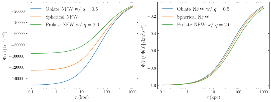
We have normalized the different profiles such that they contain the same mass within a sphere or spheroid with semi-major axis \(r\). Wee see that for the same enclosed mass, a flattened (oblate) profile gives a deeper potential well, while a prolate profile gives a shallower potential well. The right panel shows that once we normalize by the central potential, the shape of all three potentials is very similar.
As always, the gravitational field \(\vec{g} = -\nabla \Phi\) and is therefore given by
where
For axisymmetric spheroids, we obtain somewhat simpler similar expressions. E.g., for the oblate spheroids of Equation \eqref{eq-triaxialgrav-pot-oblate}, we have that
where we have set the arbitrary constant \(a_0\) to zero and we now have that
Thus, it is clear that for any density distribution that is constant on similar triaxial ellipsoids, we can compute the gravitational field using a simple one-dimensional quadrature.
From the radial component of the gravitational field at \(z=0\), we can then also determine the circular velocity curve
because \(m = R/\sqrt{\tau+1}\) in this case. We can also write this as an integral over \(m\) instead of \(\tau\) as
It is easy to see that this reduces to \(v_c^2 = GM(<r)/r\) for a spherical distribution (\(e = 0\) and \(q=1\)). For mildly-flattened systems with \(e \ll 1\) we have that \(me \ll R\) and we can Taylor expand the integrand in Equation \eqref{eq-triaxialgrav-vcirc-oblate-2} as
where \(M(<R)= 4\pi\,q\,\int_0^R\mathrm{d}m\,m^2\,\rho(m)\) is the mass within the spheroid with semi-major axis \(R\). We can also write this as
where the dimensionless function \(X(R)\) is given by
This is manifestly positive for any density distribution, so we arrive at the general result that the circular velocity at a given radius increases when we flatten any spherical mass distribution by squashing it down (i.e., conserving mass from a sphere with radius \(R\) to a spheroid of semi-major axis \(R\)). To get a better sense of \(X(R)\), we can compute it for a few example density distributions. The simplest case is for a constant density, for which
while for any power-law \(\rho(m) \propto m^{-\alpha}\)
For more complex distributions such as the Hernquist profile from Chapter 3.4.6
or the NFW profile
where in both expressions \(\tilde{R} \equiv R/a\), with \(a\) the profile’s scale radius. The following figure shows \(X(R)\) for a few different density profiles:
[19]:
figsize(7,5)
Rs= numpy.linspace(0.,12,101)
def XR_power(R,alpha=0):
    return (3.-alpha)/(5.-alpha)*R**0
def XR_Hernquist(R):
    return (2*(1.+R)**2.*(2.5+R-(5.+6.*R)/(2.*(1.+R)**2)-3.*numpy.log(1.+R)))/R**4.
def XR_NFW(R):
    return ((R-3)*R**2-6*R+6*(1+R)*numpy.log(1+R))/(2*R**2*((1+R)*numpy.log(1+R)-R))
plot(Rs,XR_power(Rs,alpha=0.),label=r'$\rho(m) \propto \mathrm{constant}$')
plot(Rs,XR_power(Rs,alpha=2.),label=r'$\rho(m) \propto m^{-2}$')
plot(Rs,XR_Hernquist(Rs),label=r'$\rho(m) = \mathrm{Hernquist}$')
plot(Rs,XR_NFW(Rs),label=r'$\rho(m) = \mathrm{NFW}$')
ylim(0.,.7)
xlabel(r'$R$')
ylabel(r'$X(R)$')
legend(frameon=True,fontsize=17.,facecolor='w',framealpha=0.75,edgecolor='None');
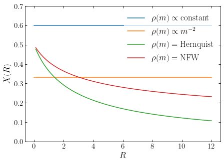
A reasonable value for many galactic density profiles is therefore \(X(R) \approx 1/3\), so we have that approximately
where \(v_{c,\mathrm{sphere}}(R)\) is the circular velocity if the mass were distributed spherically and \(R\) is the coordinate along the major axis. As an example of this approximation, we can compare it to the exact calculation for a flattened NFW profile for a Milky-Way-like NFW halo at three different radii (the same example halo that we used above):
[20]:
from galpy.potential import TriaxialNFWPotential, NFWPotential
# Base spherical NFW Potential
np= NFWPotential(mvir=1,conc=8.37,
                   H=67.1,overdens=200.,wrtcrit=True,
                   ro=8.,vo=220.)
# We will need to define the oblate versions using the amp parameter
# of the NfW profile in galpy, so we need to figure that out in
# internal coordinates
base_amp= 16.*numpy.pi*np.a**3.*np.dens(np.a,0)*np._ro**3.*u.kpc**3.
es= numpy.linspace(0.,1,41)
qs= numpy.sqrt(1-es**2.)
Rs= numpy.array([0.25,1.,10.])
vcs= numpy.zeros((len(es),len(Rs)))*u.km/u.s
for ii,e in enumerate(es):
    # to conserve mass, need to divide base_amp by q
    tp= TriaxialNFWPotential(amp=base_amp/qs[ii],a=np.a,c=qs[ii],
                            ro=8.,vo=220.)
    vcs[ii]= [tp.vcirc(R*np.a) for R in Rs]
figsize(11,4.75)
lines= []
for ii, color in enumerate(['#1f77b4','#ff7f0e','#2ca02c']):
    subplot(1,2,1)
    lines.append(plot(es,vcs[:,ii],color=color,
                      label=r'$R = {:g}\,a$'.format(Rs[ii]) if ii != 1 else r'$R = a$')[0])
    plot(es,np.vcirc(Rs[ii]*np.a)*(1.+es**2./12./qs),'--',color=color)
    subplot(1,2,2)
    plot(qs,vcs[:,ii],color=color)
    plot(qs,np.vcirc(Rs[ii]*np.a)*(1.+es**2./12./qs),'--',color=color)
subplot(1,2,1)
xlabel(r'$e$')
ylabel(r'$v_c$')
legend(handles=lines,
       fontsize=18.,loc='upper left',frameon=False)
subplot(1,2,2)
xlabel(r'$q$')
ylabel(r'$v_c$')
from matplotlib.lines import Line2D
legend_lines= [Line2D([0],[0],color='k',),
               Line2D([0],[0],color='k',ls='--')]
legend(legend_lines,
       [r'$\mathrm{exact}$',r'$v_{c,\mathrm{sphere}}(R)\left(1+{e^2 \over 12q}\right)$'],
       fontsize=18.,loc='upper right',frameon=False)
tight_layout();
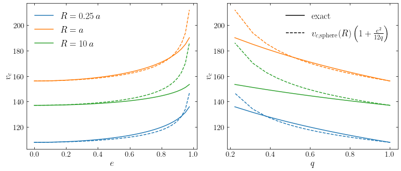
We plot the circular velocity as a function of \(e\) in the left-hand panel and of \(q\) in the right-hand panel.
For many spheroidal density profiles, we can also calculate the circular velocity using Equation \eqref{eq-triaxialgrav-vcirc-oblate-2} analytically. For example, for the NFW profile (see Chapter 3.4.6) we find that
At \(R^2 < a^2e^2\), the argument of the inverse hyperbolic tangent function is imaginary, for which we can use \(\mathrm{tanh}^{-1}(z) = \tan^{-1}(iz)/i\); the square root in the denominator of this term is also imaginary in this case and the result is a real number. Codes that implement operations on complex numbers can directly use Equation \eqref{eq-triaxialgrav-vcirc-nfw}. We can use this result to compare the rotation curves of oblate and prolate NFW halos if they contain the same amount of mass as a function of semi-major axis, using the same Milky-Way-like NFW halo as above:
[91]:
from galpy.potential import NFWPotential
def vcirc_NFW(R,q,amp=1.,a=1.):
    """Circular velocity for a spheroidal NFW profile"""
    e2= 1.-q**2.
    R2a2e2= (R**2.-a**2.*e2)*(1.+0J) # Make use of complex arithmetic!
    return numpy.sqrt(4.*numpy.pi*amp*a**3*q*R/R2a2e2\
         *((numpy.arctanh(R/numpy.sqrt(R2a2e2))
            -numpy.arctanh((R+a*e2)/q/numpy.sqrt(R2a2e2)))*R/R2a2e2**0.5
           +(a*(q-1.)-R)/(R+a)))
# Base spherical NFW Potential
np= NFWPotential(mvir=1,conc=8.37,
                   H=67.1,overdens=200.,wrtcrit=True,
                   ro=8.,vo=220.)
# We will need to define the oblate/prolate versions using the amp
# parameter of the NfW profile in galpy, so we need to figure that
# out in internal coordinates
base_amp= np.dens(np.a,0,use_physical=False)*4.
qs= [1e-16,0.1,0.5,0.9999,2.,4.]
Rs= numpy.linspace(0.01,250.,101)*u.kpc
figsize(10,5)
for q in qs:
    #amp = amp/q to keep mass within spheroids constant
    plot(Rs,vcirc_NFW((Rs/np._ro/u.kpc).to_value(u.dimensionless_unscaled),
                      q,amp=base_amp/q,a=np.a)*np._vo*u.km/u.s,
        label=r'$q = {}$'.format(q) if numpy.fabs(1.-q) > 0.1 and q > 0.01
         else r'$q = 0$' if numpy.fabs(1.-q) > 0.1 else r'$\mathrm{spherical}$')
xlabel(r'$R\,(\mathrm{kpc}$)')
ylabel(r'$v_c(R)\,(\mathrm{km\,s}^{-1})$')
xlim(0.,350.)
legend(fontsize=18.,frameon=False,loc=(0.73,0.3));
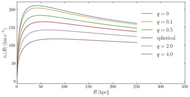
Thus, we see the expected result that flattening the mass distribution increases the rotation curve, while stretching the mass distribution along the \(z\) axis reduces it. We can in fact flatten the NFW profile all the way into a disk as shown by the \(q=0\) curve!
Further worked out expressions for the gravitational potential and field for the triaxial generalizations of the NFW and Hernquist profiles from Chapter 3.4.6 are given by Merritt & Fridman (1996).
13.2.3. The perfect ellipsoid
We have shown above that it is straightforward to compute the gravitational potential, field, and rotation curve for any ellipsoidal mass distribution using a simple one-dimensional quadrature that is easy to perform numerically. Therefore, there is little reason to use less realistic, but more tractable density distributions when studying the properties of spheroidal and ellipsoidal density distributions. However, an exception has to be made for the perfect ellipsoid (de Zeeuw 1985). Not only can the gravitational potential from Equation \eqref{eq-triaxialgrav-pot-triaxial} be worked out in terms of incomplete elliptical integrals for any combination of axis ratios \(b/a\) and \(c/a\) and the gravitational field can therefore also be obtained analytically. But the potential is also separable in ellipsoidal coordinates in such a way that the Hamilton-Jacobi equation (Chapter 4.4.3) separates and we can compute orbital actions and angles using simple one-dimensional quadratures (the potential is of so-called Staeckel form). This implies that all orbits in the perfect ellipsoid are regular (that is, non-chaotic; see Chapter 14) and that we can easily explore all of the orbits in the perfect ellipsoid because we can use the action labels to go through them. We will make use of this in Chapter 14.4 to explore orbits in triaxial potentials.
The perfect ellipsoid is defined by the density distribution on similar ellipsoids
for \(m\) given by Equation \eqref{eq-triaxial-m}. The parameter \(M\) is the total mass of the system. While the gravitational potential can be worked out in terms of incomplete elliptic integrals, the expression is quite cumbersome and we won’t give it here (see de Zeeuw 1985 for full details). At \(m \ll 1\), the density is cored, while at large \(m\), the density drops as \(m \propto m^{-4}\), leading to the finite mass. Interesting edge cases can be obtained by setting one or more of the shape parameters \((a,b,c)\) to zero. For example, for \(a=b\) and \(c=0\), the perfect ellipsoid becomes the Kuzmin disk that we discussed as a simple razor-thin disk model in Chapter 8.2.1.
We can derive the rotation curve for the perfect spheroid (i.e., \(a=b\)) using Equation \eqref{eq-triaxialgrav-vcirc-oblate-2}. First we write the density in this case as
The circular velocity is then given by
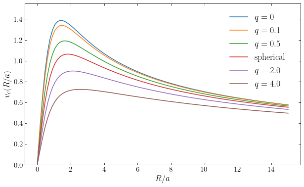
When \(q\rightarrow 0\) (and \(e \rightarrow 1\)), this becomes the circular velocity of the Kuzmin disk (Equation 8.16). Computing the rotation curve for different values of \(q\), we again see the expected trend, that more flattened distribution provide more rotational support:
[111]:
def vcirc_perfect(R,q,mass=1.,a=1.):
    """Circular velocity for a spheroidal perfect ellipsoid"""
    e2= (1.-q**2.)*(1.+0J) # Make use of complex arithmetic!
    return numpy.sqrt(2*mass*a/numpy.pi*R**2./(R**2.+a**2.*e2)**2.
                      *(numpy.sqrt(R**2./a**2.+e2)
                            *numpy.arcsin(numpy.sqrt((R**2.+a**2.*e2)/(R**2.+a**2.)))
                        -q*(R**2.+a**2.*e2)/(R**2.+a**2.)))
mass= 5
a= 1.
qs= [1e-16,0.1,0.5,0.9999,2.,4.]
Rs= numpy.linspace(0.01,15*a,101)
figsize(10,6)
for q in qs:
    plot(Rs/a,vcirc_perfect(Rs,q,mass=mass,a=a),
        label=r'$q = {}$'.format(q) if numpy.fabs(1.-q) > 0.1 and q > 0.01
         else r'$q = 0$' if numpy.fabs(1.-q) > 0.1 else r'$\mathrm{spherical}$')
xlabel(r'$R/a$')
ylabel(r'$v_c(R/a)$')
ylim(0.,1.55)
legend(fontsize=18.,frameon=False,loc=(0.73,0.45));
13.3. Multipole and basis-function expansions
In the previous section, we demonstrated that it is in fact quite straightforward to compute the gravitational potential, field, and rotation curve for any spheroidal or ellipsoidal mass distribution. However, as we saw in Section 13.1, many elliptical galaxies and likely all dark-matter halos have shapes and/or orientations that change with radius. To model such systems, we need more general methods for solving the Poisson equation than we have discussed so far. We already discussed one such solution in Chapter 8.3.5 that works best for disky mass distributions, but it involves difficult-to-work with Bessel functions. As such, this solution is not that useful in practice except for models with additional symmetries or constraints that simplify the expression substantially. In this section, we will look at a few different ways to solve the Poisson equation in full generality that are also useful in practice. For full numerical N-body work, we will discuss the solution of the Poisson equation in Chapter 19.1.
Because the Poisson equation (3.2) is linear, a general approach—which we have already taken many times!—is to break up the density into a (possibly infinite) sum of additive contributions, solve for the potential of each contribution, and add up all of the resulting potentials to obtain the full gravitational potential. We followed this approach in the previous section to determine the potential of an oblate spheroid by decomposing it into an infinite sequence of thin oblate shells. But the density constituents do not have to be simple shells, we simply want the density decomposition to be general and easy to compute, and for the Poisson equation to be easily solvable for each density contribution. For example, in Chapter 8.3.2, we determined the gravitational potential of an axisymmetric, razor-thin disk by breaking the surface density up into contributions proportional to \(k\,J_0(kR)\), which is general because of the Fourier-Bessel theorem.
In all of the methods that we discuss in this section, we will obtain the gravitational potential \(\Phi(\vec{x})\) by expanding the density \(\rho(\vec{x})\) into a complete set of basis functions \(\rho_{\vec{n}}(\vec{x})\) as
where each basis function has a solution \(\Phi_{\vec{n}}(\vec{x})\) of the Poisson equation
Using the linearity of the Poisson equation, we then obtain the gravitational potential corresponding to \(\rho(\vec{x})\) as
Note that while we write a summation sign here, one or more of the dimensions may be integrated over instead of summed if a continuous basis-function set is used. For example, in the multipole-expansion method that we discuss in Section 13.3.1 below, the radial part of the density and potential is an integral over infinitesimally-thin shells.
The Poisson equation is a partial differential equation that is particularly suited to solving by a basis function approach, because:
The Lapace operator \(\nabla^2\) is Hermitian (see below for proof); this implies that eigenfunctions of the operator—functions \(f(\vec{x})\) for which \(\nabla^2 f(\vec{x}) \propto f(\vec{x})\) analogous to eigenvectors in linear algebra—are orthogonal (see proof below). Typically, the eigenfunctions are a manifestly complete basis set for the space of functions under consideration—smooth functions that are well-behaved on the boundary of the volume being considered. In the methods described in this section, completeness is guaranteed by Sturm-Liouville theory.
The Poisson equation can be solved using the separation-of-variables technique in a variety of different coordinate systems (e.g., cartesian, cylindrical, spherical, oblate/prolate spheroidal, ellipsoidal; see Section 13.2). This provides a convenient way to obtain eigenfunctions of the Laplace operator (or other orthogonal sets of complete basis functions).
To prove the statements in the first bullet point above, we define the inner product \(\langle f,g\rangle\) of two functions \(f\) and \(g\) on \(\mathbb{R}^k\) as \(\langle f,g\rangle = \int\mathrm{d} \vec{x}\, f^*(\vec{x})\,g(\vec{x})\), where \(f^*(\vec{x})\) denotes the complex conjugate of \(f(\vec{x})\). We can then show that the Laplacian is Hermitian (at least if the functions and their gradients go to zero at infinity), that is, that \(\langle f,\nabla^2 g\rangle = \langle \nabla^2 f, g\rangle\), because
where we have used the definition of the Laplacian \(\nabla^2 = \mathrm{div}\,\vec{\nabla}\) twice and used multi-dimensional integration by parts to obtain the third and fourth lines. Good sets of basis functions can then be found as eigenfunctions of the Laplacian, that is, functions \(f_{\vec{n}}(\vec{x})\) that satisfy \(\nabla^2 f_{\vec{n}} = \lambda_{\vec{n}}\,f_{\vec{n}}\) (this equation is also known as the Helmholtz equation). Because the Laplacian is Hermitian, these basis functions are orthogonal, since then
and therefore \(\langle f_{\vec{n}},g_{\vec{n}'}\rangle =0\) if \(\lambda_{\vec{n}} \neq\lambda_{\vec{n}'}\); if an eigenvalue has a multiplicity larger than one, then the eigenfunctions for that eigenvalue can be orthogonalized using Gram-Schmidt orthogonalization. We can always define the eigenfunctions such that \(\langle f_{\vec{n}},f_{\vec{n}}\rangle = 1\) and the eigenfunctions are then orthonormal; let’s denote them as \(\rho_{\vec{n}}\) in that case. Eigenfunctions provide a convenient basis set, because the density can then be decomposed in the form of Equation \(\eqref{eq-dens-basis-expansion}\) by computing
To demonstrate that the set of eigenfunctions forms a complete basis function set requires details about the ordinary differential equations obtained using the separation-of-variables approach. Often, these differential equations will be of the Sturm-Liouville type and we can apply Sturm-Liouville theory (Courant & Hilbert 1953; Zettl 2010): this theory states that the eigenfunctions of Sturm-Liouville-type differential equations form a complete basis.
13.3.1. Multipole expansions
As a first application of the basis-function-expansion approach, we work out the standard multipole-expansion method of decomposing any density field into an infinite sequence of spherical shells with non-uniform densities. It’s obvious that any density distribution can be decomposed in this way and for elliptical galaxies and dark matter halos that are not too far from spherical it works quite well. Similar to how we proceeded in the Section 13.2, we first solve for the potential of a single thin, non-uniform shell and then compute the full potential by integrating over all shells. Everywhere outside of the shell, the Poisson equation reduces to the Laplace equation \(\nabla^2 \Phi = 0\) and we can therefore again obtain the full potential by solving the Laplace equation inside and outside of the shell in question and matching them at the radius of the shell using the appropriate boundary conditions.
The thin spherial shell with non-uniform density has a density in spherical coordinates \(\rho(r,\phi,\theta) = \delta(r-a)\,\sigma(\phi,\theta)\), where \(\sigma(\phi,\theta)\) is the surface density of the shell. To solve the Poisson equation for this density, we can follow the approach introduced above, but on the sphere rather than in three dimensions: we decompose \(\sigma(\phi,\theta)\) into basis functions, which we will suggestively denote as \(Y_l^m(\theta,\phi)\) and then solve the Poisson equation \(\nabla^2 \Phi = 4\pi G\,\sigma_{lm}\,\delta(r-a)\,Y_l^m(\theta,\phi)\) for each basis-function contribution, where \(\sigma_{lm}\) are expansion coefficients. To obtain a suitable set of basis functions \(Y_l^m(\theta,\phi)\) on the sphere, we look for eigenfunctions of the Laplace operator on the sphere using the separation-of-variables approach, that is functions \(\Phi(\phi,\theta) = F_{\vec{n}}(\phi)\,T_{\vec{n}}(\theta)\) that satisfy (using the Laplacian from Equation A.12 without the radial first term and with \(r=1\) in the other terms)
where \(\vec{n}\) is a vector indexing the eigenfunctions that we will determine as part of the solution. Substituting \(\Phi(\phi,\theta) = F_{\vec{n}}(\phi)\,T_{\vec{n}}(\theta)\) and bringing all of the \(\phi\) dependence to the right-hand side of the equation, we find
Because the left-hand side only depends on \(\theta\) and the right-hand side only depends on \(\phi\), both sides must equal a constant, say \(m^2\). The right-hand side then leads to the following equation
with solutions
Because \(F_{\vec{n}}(\phi+2\pi)= F_{\vec{n}}(\phi)\), we have that \(e^{i2\pi\,m} = 1\), and therefore \(m\) needs to be an integer: \(m = 0,\pm1,\pm2,\ldots\).
The left-hand side of Equation \(\eqref{eq-poisson-separate-spherical-firststep}\) becomes
If we write this equation in terms of \(x = \cos \theta\), we obtain
If we write \(\lambda_{\vec{n}} = -l(l+1)\), this is the Legendre differential equation. The solutions are given by the associated Legendre polynomials of the first kind \(P_l^m(x)\) and those of the second kind \(Q_l^m(x)\). For a physically-reasonable solution, we require that the solution remains finite at the poles \(\theta = 0,\pi\) or \(x=\pm1\). All Legendre functions of the second kind and all Legendre functions of the first kind with non-integer \(l\) diverge at at least one of \(x=-1\) or \(x=+1\). Therefore, physically-reasonable solutions are given by \(P_l^m(x)\), where \(l\) is an integer. These solutions further only exist if \(l \geq |m|\), which further restricts the solutions \(F_{\vec{n}}(\phi)\) to those satisfying this constraint. Finally, the Legendre differential equation is invariant under the transformation \(l \rightarrow -l-1\); therefore we only need to consider non-negative \(l\) to build a basis set (\(P_{-l}^m[x] = P_{l-1}^m[x]\)). Thus, we have that \(T_{\vec{n}}(\theta) = P_l^m(\cos \theta)\) with \(l\geq 0\) and \(|m| \leq l\).
This set of solutions \(T_{\vec{n}}(\theta)\,F_{\vec{n}}(\phi)\) often gets written in terms of a single two-dimensional function \(Y_l^m(\theta,\phi)\) known as spherical harmonics defined as
The normalization of these is chosen such that these functions are orthonormal, that is
and as we have shown, they are eigenfunctions of the two-dimensional, spherical Laplacian that satisfy
Because of the orthonormality of spherical harmonics, we can then easily decompose a shell’s non-uniform surface density \(\sigma(\phi,\theta)\) as
where the coefficients \(\sigma_{lm}\) are given by
Because the differential equations \eqref{eq-triaxialgrav-sphereFphi-diffeq} and \eqref{eq-triaxialgrav-sphereTtheta-diffeq} are of the Sturm-Liouville type, their set of solutions forms a complete basis for all smooth functions on the sphere and we can therefore decompose any smooth surface density in terms of spherical harmonics.
Now that we have decomposed the surface density of the non-uniform shell, we can return to solving the three-dimensional Poisson equation and we solve it for each \((l,m)\) component of the shell separately before summing over all \((l,m)\) contributions. That is, we solve
Because the \(Y_l^m(\theta,\phi)\) are eigenfunctions of the Laplacian that satisfy \(\nabla^2 Y_l^m(\theta,\phi) = -l(l+1) Y_l^m(\theta,\phi)\), we can find the solution of this equation as \(\Phi = R(r)\,Y_l^m(\theta,\phi)\), where \(R(r)\) satisfies (using the Laplacian in spherical coordinates from Equation A.12)
We can solve this equation by solving it at \(r < a\) and \(r > a\) and applying the appropriate boundary condition at \(r=a\). At \(r \neq a\), we have that
which has the general solution
Thus, inside the shell, we have that \(R(r) = A_{\mathrm{in}}\,r^l + B_{\mathrm{in}}\,r^{-(l+1)}\), while outside the shell \(R(r) = A_{\mathrm{out}}\,r^l + B_{\mathrm{out}}\,r^{-(l+1)}\). We set \(A_{\mathrm{out}} = 0\) such that \(R(r) \rightarrow 0\) (and thus \(\Phi(r,\phi,\theta) \rightarrow 0\)) when \(r \rightarrow \infty\). The radial component of the gravitational field is \(-Y_l^m(\theta,\phi)\,\mathrm{d} R / \mathrm{d} r\) and Gauss’s theorem (Chapter 3.2) then states that
where \(M(<r)\) is the enclosed mass within a radius \(r\). When \(r < a\), \(M(<r) = 0\) and the right-hand side of this equation should therefore vanish. The first term in the integrand always does, because \(l\,\int_0^\pi\mathrm{d}\theta\,\sin\theta\,\int_0^{2\pi}\mathrm{d}\phi\,Y_l^{m}=0\) for all \((l,m)\). The second term doesn’t, because it diverges as \(r^{-l}\) as \(r \rightarrow 0\). Therefore, we must set \(B_{\mathrm{in}}=0\) to satisfy Gauss’s theorem. Because no work is done when passing through an infinitesimally-thin shell, the potential at \(r=a\) needs to be continuous and therefore \(A_{\mathrm{in}}\,a^l = B_{\mathrm{out}}\,a^{-(l+1)}\) or \(B_{\mathrm{out}} = A_{\mathrm{in}}\,a^{2l+1}\). Finally, to determine \(A_{\mathrm{in}}\) we integrate the Poisson equation over an infinitesimal volume that encompasses a part of the spherical shell; similar to the derivation of Equation (8.12) that relates the vertical field and the surface-density for a razor-thin disk, we have in this case that
Multiplying this equation by \(Y_l^{m *}(\theta,\phi)\) and integrating over \((\phi,\theta)\) using \(\Phi_{\mathrm{in/out}} = R(r)_{\mathrm{in/out}}\,Y_l^m(\theta,\phi)\) and the orthonormality condition from Equation \eqref{eq-triaxialgrav-spherharm-ortho}, we find that
or using that \(B_{\mathrm{out}} = A_{\mathrm{in}}\,a^{2l+1}\)
Thus, the potential of a spherical shell with radius \(a\) and with non-uniform surface density \(\sigma_{lm}\,Y_l^{m}(\theta,\phi)\) is given by
For a uniform shell, we recover Newton’s shell theorems from Chapter 3.2: \(\sigma_{00}\,Y_0^{0}(\theta,\phi) = M/(4\pi\,a^2)\) in this case and therefore (a) the potential within the shell is constant and equal to \(-4\pi G\,a\,M/(4\pi\,a^2) = -GM/a\) and (b) outside of the shell, the potential is \(-4\pi G\,a\,M/(4\pi\,a^2)\,(a/r) = -GM/r\).
Using the decomposition from Equation \eqref{eq-triaxialgrav-shell-decompose-1}, we then immediately arrive at the gravitational potential of a spherical shell with an arbitrary surface density \(\sigma(\phi,\theta)\)
At large distances from the shell, the monopole (\(l=0\)) always dominates and higher-order multipoles decay faster than lower-order ones. This makes physical sense because far away from a shell, its detailed structure should become unimportant and the potential should approach that of a point mass.
For an extended body, we can decompose the density \(\rho(r,\phi,\theta)\) into a set of shells as (using \(a\) to denote the \(r\) coordinate)
where the coefficients \(\rho_{lm}(a)\) are given by
This corresponds to an infinite series of shells with surface density expressed in spherical harmonics \(\sigma_{lm} = \rho_{lm}\mathrm{d}a\) and we can thus obtain the full potential by integrating over all shells. This gives
For a spherical density we have that \(\rho_{00}(a)\,Y^0_0(\theta,\phi) = \rho(a)\) and therefore the expression simplifies to that for the potential of a spherical density (Equation 3.28). Equation \eqref{eq-triaxialgrav-multipole-potential} is the multipole expansion of the gravitational potential, with the \((l,m) = (0,0)\) term the monopole, the \(l=1\) terms are dipole terms, the \(l=2\) terms are quadrupole terms, \(l=3\) terms are octupole terms, \(l=4\) terms are hexadecapole terms, and so on. If we put everything together, computing the gravitational potential through this multipole expansion is quite complicated, because it involves a triple integral and a double sum. However, the situation is not as bad as it sounds because (i) we generally do not need to go to very high multipole orders (large \(l\) and \(|m|\)) to get a close match to the density, (ii) for tasks like orbit integration, the multipole coefficient functions \(\rho_{lm}(a)\) only need to be computed once, and (iii) because spherical harmonic decompositions are so common in many areas of science, fast numerical codes exist to efficiently perform the integrals over \((\phi,\theta)\) and sums over \((l,m)\).
We have worked out the multipole expansion here in terms of spherical harmonics and an expansion in terms of non-uniform, spherical shells. However, we could have similary expanded the density in terms of a different set of orthogonal functions, for example, as a set of non-uniform spheroidal or ellipsoidal shells (using, e.g., oblate or prolate spheroidal harmonics). For galaxies or dark-matter halos that are close to having a constant shape or orientation, this could create a more compact representation of the gravitational potential as fewer multipole terms would be needed to attain a given accuracy in the density representation. But in practice these methods are not used in galactic astrophysics, largely because the generalizations of the spherical harmonics that are required are not a standard part of an astrophysicist’s toolbox. These methods are used in situations where very high-precision in the gravitational field is required, for example, for the Earth’s gravitational field, and planets and asteroids in the solar system that one wants to, for example, land spacecraft on (e.g., Hofmann-Wellenhof & Moritz 2005; Maus 2010; Fukushima 2014).
13.3.2. Basis-function expansions
In the multipole-expansion method from the previous section, we expand densities and potentials using a countable set of basis-functions in two dimensions combined with a continuous set in the third dimension. However, for smooth density distributions, we can replace the continuous set with a countable set of complete basis functions in the third dimension as well and obtain the potential as a three-dimensional sum. This is what we will refer to as a basis-function expansion, even though the multipole expansion described above also uses basis functions.
Following the approach we have followed in the previous section to derive spherical harmonics as a complete, orthonormal basis set of smooth functions on the sphere, the obvious way to create a three-dimensional set of basis functions is to look for eigenfunctions of the three-dimensional Laplace operator using the separation of variables approach. Similar to what we did above, we look for functions functions \(\Phi(r,\phi,\theta) = R_{\vec{n}}(r)\,F_{\vec{n}}(\phi)\,T_{\vec{n}}(\theta)\) that satisfy
where \(\vec{n}\) is again a vector indexing the eigenfunctions that we will determine as part of the solution and where \(\lambda_{\vec{n}}\) are to-be-determined eigenvalues. Because it will be useful later on, to work out this equation we generalize it to \(\Phi(r,\phi,\theta) = U_{\vec{n}}(r)\,F_{\vec{n}}(\phi)\,T_{\vec{n}}(\theta)\) and work out \(\nabla^2 \left[U_{\vec{n}}(r)\,F_{\vec{n}}(\phi)\,T_{\vec{n}}(\theta)\right] = \lambda_{\vec{n}}\,R_{\vec{n}}(r)\,F_{\vec{n}}(\phi)\,T_{\vec{n}}(\theta)\); eigenfunctions are then obtained by additionally requiring that \(U_{\vec{n}}(r) \equiv R_{\vec{n}}(r)\). Using the Laplacian in spherical coordinates from Equation (A.12), we can work out Equation \eqref{eq-triaxialgrav-3dlaplace-eigenfunctions} as
This equation is similar to Equation \eqref{eq-poisson-separate-spherical-zerothstep} above and we can follow the usual approach of bringing all dependence on a single coordinate dimension on one side and the remaining coordinate dimensions to the other side. Similar to how we handled Equation \eqref{eq-poisson-separate-spherical-zerothstep}, we can bring all \(\phi\) dependence to the right-hand side and all \((r,\theta)\) dependence to the left hand-side and both sides have to then equal a constant that we again call \(m^2\). This again leads to Equation \eqref{eq-triaxialgrav-sphereFphi-diffeq} for \(F(\phi)\) with the solution of Equation \eqref{eq-triaxialgrav-sphereFphi-solution}. Following the same approach of separating coordinate dimensions for the \((r,\theta)\) part of the separated equation leads to
Again, because the left-hand side only depends on \(r\) and the right-hand side only depends on \(\theta\), both sides need to be equal to a constant, say \(l(l+1)\). The right-hand side then gives the following equation for \(T_{\vec{n}}(\theta)\)
This is the same differential equation as Equation \eqref{eq-triaxialgrav-sphereTtheta-diffeq-0} from the previous section if we set \(\lambda_{\vec{n}} = -l(l+1)\) in that equation and the solution is therefore again given in terms of associated Legendre polynomials. The combination \(T_{\vec{n}}(\theta)\,F_{\vec{n}}(\phi)\) is therefore again equal to the spherical harmonics \(Y_l^m(\theta,\phi)\) and two dimensions of the eigenvalue vector \(\lambda_{\vec{n}}\) are therefore given by the integers \((l,m)\) that satisfy \(l \leq 0\) and \(|m| \leq l\). Finally, we turn to the left-hand side of Equation \(\eqref{eq-poisson-separate-spherical-secondstep}\), which gives an ordinary differential equation for the radial part of the basis
If we require \(U_{\vec{n}}(r) \equiv R_{\vec{n}}(r)\) such that we find eigenfunctions, this equation is a form of the defining equation (B.25) of spherical Bessel functions (see Appendix B.1.2) and the basis functions can therefore be written in terms of spherical Bessel functions (e.g., Weinberg 1999). While spherical Bessel functions provide a complete basis (their defining differential equation is of the Sturm-Liouville type), these are oscillating functions that on their own do not well represent a galactic mass distribution.
If we were to use Bessel functions, we would require a large number of expansion coefficients to represent the density. Without requiring that \(U_{\vec{n}}(r)\) is an eigenfunction, however, we have much greater flexibility in finding a complete set of functions that solves Equation \(\eqref{eq-poisson-separate-spherical-radial-basis}\). A general approach is to find solutions where the lowest-order basis-function is a realistic galactic potential–density pair \([\Phi_0(r),\rho_0(r)]\), positing a general solution of the form
(e.g., Weinberg 1999; Hernquist & Ostriker 1992), where the factor of \(\sqrt{4\pi}\) is introduced to cancel \(Y_0^0 = 1/\sqrt{4\pi}\) in order to make the lowest-order function the \([\Phi_0(r),\rho_0(r)]\) pair. Plugging the radial part of this form into Equation \(\eqref{eq-poisson-separate-spherical-radial-basis}\), we get
For any choice of \([\Phi_0(r),\rho_0(r)]\), this equation can be written in Sturm-Liouville form and the solutions \(U_{nl}(r)\) therefore always provide a complete, orthogonal basis for the space of functions under consideration. Because of this orthogonality, decomposing any density \(\rho(r,\phi,\theta)\) into \(\rho_{nlm}(r,\phi,\theta)\) components is straightforward
where the expansion coefficients are given by
where \(\Phi_{nlm}^*\) is the complex conjugate of \(\Phi_{nlm}\) (in practice, by combining terms with opposite-sign \(m\), we can compute two sets of real coefficients by replacing \(e^{im\phi}\) with either of \(\cos[m\phi]\) and \(\sin[m\phi]\)). The gravitational potential is then given by
A general approach to coming up with complete sets of basis functions that can be used to represent an arbitrary density is then to choose the \([\Phi_0(r),\rho_0(r)]\) pair to closely resemble to overall radial profile of the density one wants to model and to then solve Equation \eqref{eq-poisson-separate-spherical-radial}. This approach combines the advantages of using eigenfunctions with the flexibility to choose physically-meaningful radial basis functions and if the lowest-order model is a close match to the full density, few terms are necessary in the expansion to accurately represent the density. Equation \(\eqref{eq-poisson-separate-spherical-radial}\), however, in general cannot be solved in terms of known functions and for most \([\Phi_0(r),\rho_0(r)]\) pairs one therefore has to solve it numerically (e.g., for the NFW profile; Dai et al. 2018). Because Sturm-Liouville problems are so common, software exists to compute such numerical solutions efficiently (see, e.g., Weinberg 1999 for an application of this). From the definition, we know that \(U_{00}(r) = 1\) and \(\lambda_{00} =1\).
For computational convenience and speed, it is useful to have analytical basis-function sets and Equation \(\eqref{eq-poisson-separate-spherical-radial}\) can in fact be solved for two important cases: (a) if \([\Phi_0(r),\rho_0(r)]\) is the Plummer potential–density pair (see Chapter 3.4.3; Clutton-Brock 1973) or (b) when \([\Phi_0(r),\rho_0(r)]\) is the Hernquist potential–density pair (see Chapter 3.4.6; Hernquist & Ostriker 1992). These provide good sets of basis functions to represent the potential of globular clusters (for the Plummer-based set) and dark-matter halos and elliptical galaxies (for the Hernquist-based set). Because it is widely used in galactic dynamics and to further illustrate the approach, we briefly discuss the Hernquist & Ostriker (1992) method based on the Hernquist potential–density pair, which the authors refer to as the self-consistent field method.
For convenience, we work with a unit mass Hernquist profile with scale radius \(a=1\); because a non-unit mass is a simple rescaling of the density and potential and because a non-zero scale radius simply scales all positions as \(r/a\), it is straightforward to apply the formulae below in these cases. The Hernquist potential–density pair is then derived from Equations (3.58), (3.60), and (3.62)
The main task at hand is then to solve Equation \eqref{eq-poisson-separate-spherical-radial}. To make headway in this, Hernquist & Ostriker (1992) posited that the \(U_{nl}(r)\) have the following form
This form is inspired by the multipole-expansion that we discussed above (e.g., Equation \ref{eq-triaxialgrav-shell-potential}), where the potential is \(\propto r^l\) at small \(r\) and \(\propto 1/r^{l+1}\) at large \(r\). If \(W_{0l}(\xi)=1\), then the lowest-order radial basis functions have this behavior at \(r \ll 1\) and \(r \gg 1\), respectively. The unknown functions \(W_{nl}(\xi)\) then represent deviations from this basic behavior through the higher-order radial basis functions. We write \(W_{nl}\) as a function of a coordinate \(\xi(r)\) that is determined by the requirement that the differential equation for \(W_{nl}\) that results from plugging Equation \eqref{eq-triaxialgrav-scf-Uansatz} into Equation \eqref{eq-poisson-separate-spherical-radial} is of known form. Hernquist & Ostriker (1992) show that it is useful to define \(\xi(r)\) as
because then \eqref{eq-poisson-separate-spherical-radial} becomes
where we have defined \(K_{nl} = \lambda_{nl}/[2\pi]\). This may not seem simple, but it is equivalent to the equation defining the Gegenbauer (or ultraspherical) polynomials \(C_n^\alpha(\xi)\) if \(\alpha = 2l+3/2\) and \(K_{nl}\) is given by
Thus, the full orthogonal basis-function set is
The expansion coefficients can be computed using Equation \eqref{eq-triaxialgrav-bfe-coeffs}.
The approach we have followed so far in ths section works well for densities that are not too far from spherical (like elliptical galaxies and dark matter halos). But it does not work well for disks, which are so far from spherical that they would require very high order in \(l\) to be well-described by an expansion in terms of spherical harmonics. Thus, to represent disk potentials through basis-function expansions, it is necessary to come up with different sets of basis functions. Indeed, many of the first applications of basis-function expansions in galactic dynamics were for disks (e.g., Clutton-Brock 1972; Kalnajs 1976). These first applications were for the gravitational field within a razor-thin disk, where the separation-of-variables approach to the Helmholtz equation in two dimensions leads to basis functions that are combinations of Bessel functions for the radial component and \(e^{im\phi}\) for the azimuthal component (this can be shown by following a similar approach as we took in Chapter 8.3.5). Bessel functions are again not realistic galactic components, so we can follow a similar approach as we did in the three-dimensional case above of finding radial potential-density pairs for which the lowest-order component is a realistic disk density and that form a complete basis.
The situation is trickier for thick disks (that is, not razor-thin in this context). For those we could again look for a complete set of basis functions by solving the Helmholtz equation using the separation-of-variables approach in cylindrical coordinates. This leads to basis functions that are combinations of (i) Bessel functions for the radial component, (ii) \(e^{im\phi}\) for the azimuthal component, and (iii) \(e^{ihz}\) for the vertical component. However, the vertical profile of disks is not well described as \(e^{ihz}\) and, thus, we now have the unfortunate situation where two of the dimensions of our basis functions do not describe realistic galactic density profiles. The approach that we followed above of replacing the offending radial eigenfunctions with a complete set of potential-density pairs is now much harder to follow, because we need to replace both the radial and vertical eigenfunctions. Earn (1996) describes an approach of this form, but it leads to a complete set of basis functions that is not orthogonal. In that case, we cannot compute expansion coefficients using an expression like Equation \eqref{eq-triaxialgrav-bfe-coeffs}, but instead we need to solve for the coefficients \(A_{\vec{n}}\) by solving the equation
where the matrix \(M_{\vec{n}\vec{m}}\) is given by
Alternatively, we can orthogonalize a non-orthogonal set using Gram-Schmidt orthogonalization, but in the end the computational cost is similar. When using a basis-function expansion method, solving for the expansion coefficients is generally not the most time-consuming step, so the fact that we now have to solve a matrix equation rather than directly computing the coefficients is not too burdensome. Aside from this complication, the basis-function expansion in terms of disky basis functions is not that different from that which we described in detail above and we refer the reader to Earn (1996) for more details. Robijn & Earn (1996) and Brown & Papaloizou (1998) give similar, related approaches.
Using a simple trick, the basis-function approach based on spherical harmonics discussed in this section can also be applied to derive the potential of general disk mass distributions, by using the basis-function expansion to describe the difference between the actual density and a good disky approximation to it. If the approximation is good enough, the difference is much closer to spherical than the original density and the difference can therefore efficiently be represented using either the multipole expansion or a basis-function expansion based on spherical harmonics. See Kuijken & Dubinski (1995) and Dehnen (1998) for more details.
Finally, we will discuss \(N\)-body modeling of galactic systems in detail in Chapter 19, but we note here that the basis-function approach was originally introduced as a way to efficiently solve the Poisson equation in \(N\)-body simulations. However, its use in this area has been quite limited. In this approach, the gravitational potential is computed from a set of \(N\) particles by computing the expansion of the density down to some relatively low-order \((n,l,m)\)—this computation can be done efficiently in \(\mathcal{O}(N)\) time (e.g., Hernquist & Ostriker 1992). While this approach conceptually solves the issue of using individual particles to represent a smooth density field, because the density is automatically smoothed by using a low-order expansion, the expansion is quite sensitive to finding the exact center of the simulation (when using the Hernquist-based expansion, the radial basis functions diverge at \(r=0\)) and to fully represent even the smooth density field, many terms in the expansion are typically required. The former issue makes this approach difficult to use for all simulations, except perhaps for those of isolated galaxies (where the center might be better defined than in, say, the simulation of a galaxy merger); the latter issue means that the \(\mathcal{O}(N)\) has a large pre-factor, which itself depends on \(N\) and, it has been argued, leads to \(\mathcal{O}(N^2)\) behavior for the full force calculation (Dehnen 2001). This is much worse than other Poisson solvers for the \(N\)-body problem that we will discuss in Chapter 19.1.
Basis-function expansions, however, have been and remain very important in analyses of perturbations to equilibrium states of galaxies, for example, to determine whether equilibrium states are stable to small perturbations.