18. Formation of dark matter halos

\label{chapter-dmhaloform}

18.1. Cosmological evolution of small perturbations

Dark matter halos—and the galaxies that reside within them—form from small seeds sown by whatever process sets the initial pattern of overdensities and underdensities in all of the components that make up the Universe. The overdensities start out as very small perturbations on top of the smooth density. They evolve under the influence of gravity and other physical processes and eventually grow so large that they form the bound, virialized objects known as dark matter halos. When the perturbations are small, their evolution can be studied using relatively simple tools, which we describe in this first section of this chapter.

18.1.1. Evolution of small cold-dark-matter perturbations

In the standard model of cosmology, dark matter is collisionless and its evolution on scales small compared to the scale of the Universe—the horizon—is therefore given by the collisionless Boltzmann equation, which we derived in Chapter 6.3. Only on the horizon scale and larger is a general relativistic description necessary and we will not discuss such perturbations in detail here. The collisionless Boltzmann equation gives the evolution of the distribution function \(f(\vec{q},\vec{p},t)\) that represents the number of dark matter particles in a given volume of phase space centered on \((\vec{q},\vec{p})\) at time \(t\). In proper coordinates \((\vec{r},\vec{u})\)—actual coordinates, not those expanding with the Universe—the Lagrangian is the regular one

\begin{equation} \mathcal{L}(\vec{r},\dot{\vec{r}},t) = \frac{m|\dot{\vec{r}}^2|}{2}-m\Psi(\vec{r},t)\,, \end{equation}

where \(\Psi(\vec{r},t)\) is the gravitational potential, because the dark matter only interacts gravitationally (we use \(\Psi\) rather than \(\Phi\), because we will later introduce \(\Phi\) as the potential due to perturbations in the density, not the full density). Because the Universe is expanding isotropically and homogeneously, it is expedient to express equations in terms of comoving coordinates—coordinates that are relative to the expanding Universe. These coordinates \(\vec{x}\) are defined by \(\vec{r} = a(t)\,\vec{x}\), where \(a(t)\) is the scale factor at time \(t\). The Lagrangian can then be written in terms of \((\vec{x},\dot{\vec{x}})\) as

\begin{equation} \mathcal{L}(\vec{x},\dot{\vec{x}},t) = \frac{m}{2}\,\left(\dot{a}\,\vec{x} + a\,\dot{\vec{x}}\right)^2-m\Psi(\vec{x},t)\,. \end{equation}

Using Lagrange’s equations from Chapter 4.3, we obtain the canonical momentum conjugate to \(\vec{x}' = \vec{x}\)—we denote this canonical coordinate pair with an apostrophe, because we will perform a further transformation to the final set of canonical coordinates):

\begin{equation} \vec{p}' = \frac{\partial \mathcal{L}}{\partial \dot{\vec{x}}} = m\,a\,\left(\dot{a}\,\vec{x} + a\,\dot{\vec{x}}\right)\,. \end{equation}

The Hamiltonian in terms of \((\vec{x}',\vec{p}')\) is given by

\begin{align} H(\vec{x}',\vec{p}',t) & = \dot{\vec{x}}'\cdot\vec{p}' - \mathcal{L}(\vec{x}',\dot{\vec{x}}',t)\\ & = m\,a\,\left(\dot{a}\,\vec{x}'\,\dot{\vec{x}}' + a\,\dot{\vec{x}}'^2\right) -\frac{m}{2}\,\left(\dot{a}\,\vec{x}' + a\,\dot{\vec{x}}'\right)^2+m\Psi(\vec{x}',t)\\ & = \frac{m\,a^2}{2}\,\dot{\vec{x}}'^2 -\frac{m}{2}\,\dot{a}^2\,\vec{x}'^2+m\Psi(\vec{x}',t) \end{align}

To further simplify this, we canonically transform \((\vec{x}',\vec{p}')\) using a generating function of the third kind \(F_3(\vec{p}',\vec{x})\) that is a function of the old momentum and the new coordinate. Specifically, we use

\begin{equation} F_3(\vec{p}',\vec{x}) = -\vec{p}'\cdot\,\vec{x} + m\,a\,\dot{a}\,|\vec{x}|^2/2\,, \end{equation}

because then the transformation equations give

\begin{align} \vec{p} & = -\frac{\partial F_3}{\partial \vec{x}} = m\,a^2\,\dot{\vec{x}}\\ \vec{x}' & = -\frac{\partial F_3}{\partial \vec{p}'} = \vec{x}\,. \end{align}

Thus, the effect of the canonical transformation is to remove the term \(\propto \vec{x}\) in the canonical momentum, while keeping the coordinate the same. The momentum is now proportional to \(\vec{v} = a\,\dot{\vec{x}}\), the peculiar velocity with respect to the expansion of the Universe. The Hamiltonian is transformed under the canonical transformation specified above as

\begin{align} H \rightarrow & H + \frac{\partial F_3}{\partial t}\\ & = \frac{m\,a^2}{2}\,\dot{\vec{x}}^2 -\frac{m}{2}\,\dot{a}^2\,\vec{x}^2+m\Psi(\vec{x},t) +\frac{m\,\dot{a}^2}{2}\,|\vec{x}|^2 +\frac{m\,a\,\ddot{a}}{2}\,|\vec{x}|^2\\ & = \frac{1}{2\,m\,a^2}\,\vec{p}^2 +m\Psi(\vec{x},t) +\frac{m\,a\,\ddot{a}}{2}\,|\vec{x}|^2\,, \end{align}

or if we define

\begin{equation} \Phi(\vec{x},t) = \Psi(\vec{x},t) + \frac{a\,\ddot{a}}{2}\,|\vec{x}|^2\,, \end{equation}

the Hamiltonian simply becomes

\begin{equation} H(\vec{x},\vec{p},t) = \frac{1}{2\,m\,a^2}\,\vec{p}^2 +m\Phi(\vec{x},t)\,. \end{equation}

Because of the second Friedmann equation, this potential \(\Phi\) is that due to the density perturbation \(\delta(\vec{x},t)\) with respect to the mean background density (and this holds even in the presence of radiation and dark energy):

\begin{equation}\label{eq-poisson-comoving-perturb} \nabla^2 \Phi(\vec{x},t) = 4\pi\,G\overline{\rho}(t)\,a(t)^2\,\delta(\vec{x},t)\,. \end{equation}

We can now write the collisionless Boltzmann equation in the comoving, canonical coordinates by using the Hamiltonian in the expression of the collisionless Boltzmann equation for general canonical coordinates from Equation (6.33):

\begin{equation}\label{eq-cbe-comoving} \frac{\partial f}{\partial t} +\frac{1}{m\,a^2}\,\vec{p}\,\frac{\partial f}{\partial \vec{x}} -m\,\frac{\partial \Phi}{\partial \vec{x}}\,\frac{\partial f}{\partial \vec{p}}=0\,. \end{equation}

We can then again derive Jeans equations like we did in Chapter 6.4. Integrating this equation over the momenta gives a continuity equation

\begin{equation}\label{eq-collisionless-continuity} \frac{\partial \delta}{\partial t} + a^{-1}\,\nabla\cdot\langle\vec{v}\rangle = 0\,, \end{equation}

where \(\nabla\) is the gradient with respect to \(\vec{x}\), \(\langle\vec{v}\rangle\) is the mean velocity, and \(\delta\) is the overdensity in the co-moving number density \(n(\vec{x})\), that is

\begin{equation} n(\vec{x}) = \overline{\rho}\,a^3\,\left(1+\delta\right)\,. \end{equation}

Similarly, multiplying Equation \(\eqref{eq-cbe-comoving}\) by \(v_i\) and integrating over all momenta gives

\begin{equation} \frac{\partial}{\partial t} \left(\left[1+\delta\right]\,\langle v_i\rangle\right)+\frac{\dot{a}}{a}\,\left(1+\delta\right)\,\langle v_i\rangle = -\frac{\left(1+\delta\right)}{a}\,\frac{\partial \Phi}{\partial x_i}-a^{-1}\,\sum_j\,\frac{\partial}{\partial x_j}\left(\left[1+\delta\right]\langle v_i\,v_j\rangle\right)\,. \end{equation}

If we then multiply the continuity equation by \(\langle v_i\rangle\) and subtract it from this equation, we obtain

\begin{equation}\label{eq-collisionless-euler} \frac{\partial \langle \vec{v}\rangle}{\partial t}+\frac{\dot{a}}{a}\,\langle \vec{v}\rangle +a^{-1}\,(\langle \vec{v}\rangle\cdot\nabla)\langle\vec{v}\rangle = -a^{-1}\,\nabla \Phi -\frac{1}{a\left(1+\delta\right)}\,\nabla\cdot \left(\left[1+\delta\right]\,\vec{\sigma}^2\right)\,, \end{equation}

where \(\vec{\sigma}^2\) is the stress tensor

\begin{equation} \sigma_{ij}^2 = \langle v_i\,v_j\rangle - \langle v_i\rangle\,\langle v_j\rangle\,. \end{equation}

The stress tensor acts as a type of pressure—in the next subsection, we derive the evolution equations for baryons and will see that this equation is the same as the Euler equation when we interpret \(\sigma_{ij}^2\) as pressure. That dark matter is cold means that its early-Universe value of \(\vec{\sigma}^2 \ll \langle \vec{v}\rangle\) and this remains so as long as \(\delta \ll 1\) (dark matter only “heats” up in this sense once it falls into a collapsing halo and then \(\delta \gg 1\)). Therefore, Equation \(\eqref{eq-collisionless-euler}\) for cold dark matter simplifies to

\begin{equation}\label{eq-collisionless-euler-cold} \frac{\partial \langle \vec{v}\rangle}{\partial t}+\frac{\dot{a}}{a}\,\langle \vec{v}\rangle +a^{-1}\,(\langle \vec{v}\rangle\cdot\nabla)\langle\vec{v}\rangle = -a^{-1}\,\nabla \Phi\,. \end{equation}

Equations \(\eqref{eq-collisionless-continuity}\) and \(\eqref{eq-collisionless-euler-cold}\) are the basic equations that govern the evolution of dark matter density fluctuations. As long as perturbations are small, they simplify to (keeping only terms linear in the perturbation; peculiar velocities are perturbative as well: \(\vec{v} \approx \delta)\) and we have then that

\begin{align}\label{eq-dm-evol-0} \frac{\partial \delta}{\partial t} + a^{-1}\,\nabla\cdot\langle\vec{v}\rangle & = 0\,,\\ \frac{\partial \langle \vec{v}\rangle}{\partial t}+\frac{\dot{a}}{a}\,\langle \vec{v}\rangle & = -a^{-1}\,\nabla \Phi\,.\label{eq-dm-evol-1} \end{align}

Taking the time derivative of the first of these we can use the second equation to substitute the mean velocity derivative. Then employing the Poisson equation \(\eqref{eq-poisson-comoving-perturb}\), we find that

\begin{equation}\label{eq-ddotdelta-dm} \frac{\partial^2 \delta}{\partial t^2} +2\,\frac{\dot{a}}{a}\,\frac{\partial \delta}{\partial t} = 4\pi\,G\,\overline{\rho}\,\delta\,. \end{equation}

For a given cosmology—which specifies \(a(t)\)—we can solve this second-order differential equation for the evolution of small perturbations of cold dark matter. Operating Equation \(\eqref{eq-dm-evol-1}\) with \(\nabla \times\) we find that

\begin{equation} \frac{\partial \nabla \times \langle \vec{v}\rangle}{\partial t}+\frac{\dot{a}}{a}\,\nabla \times \langle \vec{v}\rangle = 0\,, \end{equation}

because \(\nabla \times (\nabla \Phi) = 0\)—the curl of the gradient of scalar function is always zero. Therefore \(\nabla \times \langle \vec{v}\rangle \propto a^{-1}\) and the curl of the mean velocity field decays as the Universe expands. Because there is no source of vorticity at first order, it is therefore a good assumption that the mean velocity is curl-free and can therefore be written as the gradient of a “vector potential”.

18.1.2. Evolution of small baryonic overdensities in the Universe

\label{sec-dmhaloform-baryons}

Cold dark matter is about five times more abundant than baryonic matter, so while the formalism given above describes the evolution of the dominant matter component, baryons cannot be entirely neglected. Before discussing specific solutions to the evolution equations for cold dark matter given above, we therefore describe the evolution of baryonic perturbations.

Baryons in the early Universe are in gaseous form and they can therefore not be described by the collisionless formalism above. Because collisions are so frequent, we can approximate the baryonic component as an ideal fluid—the ideal fluid description is good as long as the mean free path is much smaller than the (cosmological) scales of interest. As above, we only consider perturbations on scales small compared to the overall size of the Universe and we can therefore use a Newtonian formalism. The evolution of a fluid is given by the continuity

\begin{equation} \frac{\partial \rho}{\partial t} + \nabla \cdot \rho\,\vec{u} = 0\,, \end{equation}

and the Euler equation

\begin{equation} \frac{\partial \vec{u}}{\partial t} + (\vec{u}\cdot \nabla)\,\vec{u} = -\frac{\nabla P}{\rho} - \nabla \Psi\,, \end{equation}

where \(P\) is the pressure and \(\Psi\) the gravitational potential. These equations are again in terms of proper position-velocity coordinates \((\vec{r},\vec{u})\) and the gradients are taken with respect to \(\vec{r}\). The relation between the density and potential is given by the Poisson equation.

As above, we express these equations in terms of comoving coordinates defined by \(\vec{r} = a(t)\,\vec{x}\) and \(\vec{u} =\dot{a}\,\vec{x}+ \vec{v}\) where \(\vec{v} = a\,\dot{\vec{x}}\) is the peculiar velocity. We again express the density in terms of the perturbation away from the mean density: \(\rho(\vec{x},t) = \overline{\rho}(t)\,\left(1+\delta(\vec{x},t)\right)\), where \(\overline{\rho}(t) \propto a^{-3}\); and also express the potential \(\Psi\) in terms of the potential perturbation \(\Phi\): \(\Psi = \Phi - a\,\ddot{a}\,|\vec{x}|^2/2\). Then the fluid equations and the Poisson equation become

\begin{align}\label{eq-baryon-evol-preeqstat-0} \frac{\partial \delta}{\partial t} + a^{-1}\,\nabla\cdot \left(\left[1+\delta\right]\,\vec{v}\right) & = 0\,,\\ \frac{\partial \vec{v}}{\partial t}+ \frac{\dot{a}}{a}\,\vec{v}+a^{-1}\,(\vec{v}\cdot \nabla)\,\vec{v} & = a^{-1}\,\nabla \Phi-\frac{\nabla P}{a\,\overline{\rho}\left[1+\delta\right]}\,,\label{eq-baryon-evol-preeqstate}\\ \nabla^2 \Phi & = 4\pi\,G\,\overline{\rho}\,a^2\,\delta\,.\label{eq-baryon-evol-preeqstat-2} \end{align}

In these equations, the spatial gradients are now with respect to \(\vec{x}\).

To solve the fluid–Poisson equations, we need one more equation: an equation of state \(P = P(\rho,T)\) that relates the pressure to the density and temperature of the gas \(T\), or equivalently, the density and specific entropy \(s\) as \(P = P(\rho,S)\). Because we believe that the Universe and perturbations within it evolve adiabatically (or isentropically), that is without changing the entropy, many of the useful equations of state simply relate pressure to density \(P = P(\rho)\); these are barotropic equations of state. Examples are those used when computing the expansion of the Universe: radiation is described by \(P = \rho\,c^2/3\), dark energy by \(P = -\rho\,c^2\), and adiabatic dust (the simplest cosmological model for dark matter and baryons) has \(P = \rho\,c_s^2\), where \(c_s\) is the sound speed, which is zero for dark matter. Because we are interested in describing the evolution of perturbations of gaseous baryons, we will consider the latter case in more detail.

If we approximate the baryonic fluid as an ideal gas, the equation of state is

\begin{equation}\label{eq-ideal-gas} P = \frac{\rho\,k_B\,T}{\mu\,m_p}\,, \end{equation}

where \(k_B\) is the Boltzmann constant, \(m_p\) is the proton mass, and \(\mu\) is the mean molecular weight in terms of the proton mass (\(\mu = 1.22\) for a primordial mixture of hydrogen and helium with a helium mass fraction of 0.24). To derive the adiabatic equation of state, we use the first law of thermodynamics relating changes in the specific internal energy \(u\) to changes in entropy and volume:

\begin{equation}\label{eq-first-thermo} \mathrm{d} u = T\,\mathrm{d} s - p\,\mathrm{d} V\,, \end{equation}

where \(V = 1/\rho\), the volume per unit mass. For particles with \(q\) degrees of freedom, the internal energy is

\begin{equation} u = \frac{q}{2}\,\frac{k_B\,T}{\mu\,m_p}\,, \end{equation}

and for a mono-atomic gas specifically, \(q=3\), such that \(u = 3 k_B T/2\). Plugging this into Equation \(\eqref{eq-first-thermo}\) and using the ideal gas law in Equation \(\eqref{eq-ideal-gas}\) we find that

\begin{equation} \frac{q}{2}\,\frac{k_B}{\mu\,m_p}\mathrm{d} T = T\,\mathrm{d} s + \frac{k_B\,T}{\mu\,m_p}\,\mathrm{d}\ln \rho\,, \end{equation}

or

\begin{equation} \mathrm{d} s= \frac{k_B}{\mu\,m_p}\left(\frac{q}{2}\,\mathrm{d} \ln T - \mathrm{d}\ln \rho\right)\,, \end{equation}

and therefore

\begin{equation} \exp\left(\frac{\mu\,m_p}{k_B}\,s\right)\propto \frac{T^{q/2}}{\rho}\,, \end{equation}

or, using Equation \(\eqref{eq-ideal-gas}\) this gives the equation of state

\begin{equation} P\propto \rho^{(q+2)/q}\,\exp\left(\frac{2}{q}\,\frac{\mu\,m_p}{k_B}\,s\right)\,. \end{equation}

For the isentropic evolution of a mono-atomic gas, we therefore have that

\begin{equation} P \propto \rho^{5/3}\,. \end{equation}

Going back to Equation \(\eqref{eq-baryon-evol-preeqstate}\), the term involving \(\nabla P\) requires

\begin{equation} \frac{\nabla P}{\overline{\rho}} = c_s^2\,\nabla \delta + \frac{2}{3}\,\left[1+\delta\right]\,T\,\nabla S\,, \end{equation}

where \(c_s\) is the sound speed

\begin{equation} c_s = \sqrt{\frac{q+2}{q}\,\frac{k_B\,T}{\mu\,m_p}}\,. \end{equation}

Equation \(\eqref{eq-baryon-evol-preeqstate}\) can then be written as

\begin{equation}\label{eq-baryon-evol-general} \frac{\partial \vec{v}}{\partial t}+ \frac{\dot{a}}{a}\,\vec{v}+a^{-1}\,(\vec{v}\cdot \nabla)\,\vec{v} = a^{-1}\,\nabla \Phi-\frac{c_s^2\,\nabla \delta}{a\,\left[1+\delta\right]}-\frac{2}{3}\,a^{-1}\,T\,\nabla S\,. \end{equation}

When baryonic perturbations are small, they evolve adiabatically—non-adiabatic changes are only significant once baryons fall into dark matter halos and shock, but at this point the perturbation is \(\delta \gg 1\). The evolution of small perturbations is therefore given by the \(\delta, \vec{v} \ll 1\) limit of Equations \(\eqref{eq-baryon-evol-preeqstat-0}\)–\(\eqref{eq-baryon-evol-preeqstat-2}\) with \(\nabla S = 0\) in which we drop all terms that are a power of two or more of the small quantities

\begin{align}\label{eq-baryon-evol-general-0} \frac{\partial \delta}{\partial t} + a^{-1}\,\nabla\cdot \vec{v} & = 0\,,\\ \frac{\partial \vec{v}}{\partial t}+ \frac{\dot{a}}{a}\,\vec{v} & = a^{-1}\,\nabla \Phi-a^{-1}\,c_s^2\,\nabla \delta\,,\label{eq-baryon-evol-general-1}\\ \nabla^2 \Phi & = 4\pi\,G\,\overline{\rho}\,a^2\,\delta\,.\label{eq-baryon-evol-general-2} \end{align}

Like we did for dark matter perturbations, we can take the time derivative of the first equation and simplify it using the second and third to obtain

\begin{equation}\label{eq-ddotdelta-with-pressure} \frac{\partial^2 \delta}{\partial t^2}+2\,\frac{\dot{a}}{a}\,\frac{\partial \delta}{\partial t} = 4\pi\,G\,\overline{\rho}\,\delta +\frac{c_s^2}{a^2}\,\nabla^2\delta\,. \end{equation}

Operating Equation \(\eqref{eq-baryon-evol-general}\) with \(\nabla \times\) we again obtain that \(\nabla \times \vec{v} = a^{-1}\)—now because all source terms on the right-hand side are gradients of scalar functions—and we can again approximate the velocity field as being curl-free. Comparing the evolution equations of cold dark matter and baryons, we notice that they are almost exactly the same, except for the pressure term in the baryonic Euler equation.

The equations we derived here apply only after baryons have decoupled from photons at recombination at \(z \approx 1100\). Before recombination baryons are coupled to photons through Thomson scattering and form a baryon-photon plasma that also behaves as an ideal fluid, but whose evolution equations have additional terms due to the coupling. After recombination, the electromagnetic interactions with photons cease and because radiation stopped being a significant component of the Universe at \(z \approx 3200\) and dark energy only becomes significant at \(z<1\), as far as baryons and dark matter care, the Universe only consists of matter. The co-evolution of cold dark matter and baryons is therefore given by the fluid-like equations for the dark matter, Equations \(\eqref{eq-dm-evol-0}\) and \(\eqref{eq-dm-evol-1}\) for the dark matter overdensity \(\delta_c\) and velocity \(\langle \vec{v}_c\rangle\), the fluid equations for the baryons, Equations \(\eqref{eq-baryon-evol-general-0}\) and \(\eqref{eq-baryon-evol-general-1}\) for the baryonic overdensity \(\delta_b\) and velocity \(\vec{v}_b\), and the Poisson equation relating the gravitational potential perturbation to the total density perturbation. If we define each components overdensity, \(\delta_c\) and \(\delta_b\), to be relative to its own mean density, then the total density perturbation is the weighted sum of the dark-matter and baryon overdensities, with weights equal to the relative matter fraction in dark matter and baryons, \(\Omega_c/\Omega_m\) and \(\Omega_b/\Omega_m\), respectively (where \(\Omega_m\) is the density parameter of all matter). The Poisson equation thus becomes

\begin{equation} \nabla^2 \Phi = 4\pi\,G\,\overline{\rho}\,a^2\,\left(\frac{\Omega_c}{\Omega_m}\,\delta_c+\frac{\Omega_b}{\Omega_m}\,\delta_b\right)\,. \end{equation}

The Poisson equation is the only equation coupling the dark matter to the baryons, because dark matter only interacts gravitationally. Because we often do not particularly care about the evolution of the peculiar velocities, the relevant evolution equations are the coupled version of the equations for the second time derivative of the density perturbation that we derived for cold dark matter and baryons

\begin{align} \frac{\partial^2 \delta_c}{\partial t^2} +2\,\frac{\dot{a}}{a}\,\frac{\partial \delta_c}{\partial t} & = 4\pi\,G\,\overline{\rho}\,\left(\frac{\Omega_c}{\Omega_m}\,\delta_c+\frac{\Omega_b}{\Omega_m}\,\delta_b\right)\,,\\ \frac{\partial^2 \delta_b}{\partial t^2}+2\,\frac{\dot{a}}{a}\,\frac{\partial \delta_b}{\partial t} & = 4\pi\,G\,\overline{\rho}\,\left(\frac{\Omega_c}{\Omega_m}\,\delta_c+\frac{\Omega_b}{\Omega_m}\,\delta_b\right) +\frac{c_s^2}{a^2}\,\nabla^2\delta_b\,. \end{align}

18.1.3. Solutions for the evolution of small matter perturbations

Now that we have derived the equations governing the evolution of small perturbations in the Universe (on scales less than the horizon scale and for baryons only after decoupling from the photons at recombination), we discuss aspects of their solution. In general, the evolution equations must be solved numerically—and this is what is done when initializing cosmological \(N\)-body simulations—but we can make some analytical headway that sheds light on the solutions.

18.1.3.1. Fourier decomposition

Because the evolution equations are linear in the perturbation for small perturbations, they are typically solved by taking the spatial Fourier transformation of the evolution equations and finding the evolution equations for the evolution of each Fourier mode. This is useful, because it removes all spatial derivatives from the equations. We decompose the density perturbation (of dark matter or baryons) as

\begin{equation} \delta(\vec{x},t) = \sum_{\vec{k}}\delta_{\vec{k}}(t)\,\exp\left(i\vec{k}\cdot\vec{x}\right)\,, \end{equation}

where we compute the coefficients \(\delta_{\vec{k}}(t)\) as the Fourier transform

\begin{equation} \delta_{\vec{k}}(t) =\frac{1}{V}\,\int_V\,\mathrm{d}\vec{x}\,\delta(\vec{x},t)\,\exp\left(-i\vec{k}\cdot\vec{x}\right)\,, \end{equation}

where \(V\) is a large volume over which the perturbation is assumed to be periodic. If we take the Fourier transform of Equation \(\eqref{eq-ddotdelta-with-pressure}\)—which by setting \(c_s = 0\) includes the cold-dark-matter case—we obtain the evolution equation for the modes \(\delta_{\vec{k}}\)

\begin{equation}\label{eq-ddotdelta-with-pressure-ink} \frac{\partial^2 \delta_{\vec{k}}}{\partial t^2}+2\,\frac{\dot{a}}{a}\,\frac{\partial \delta_{\vec{k}}}{\partial t} = 4\pi\,G\,\overline{\rho}\,\delta_{\vec{k}} -\frac{k^2\,c_s^2}{a^2}\,\delta_{\vec{k}}\,, \end{equation}

where we write \(k^2 \equiv |\vec{k}|^2\). For cold dark matter, this equation does not contain \(\vec{k}\) and the evolution of each mode \(\delta_{\vec{k}}\) is identical: perturbations on all scales grow or decay at the same rate. For baryons we can re-write Equation \(\eqref{eq-ddotdelta-with-pressure-ink}\) as

\begin{equation}\label{eq-ddotdelta-with-pressure-ink-baryons} \frac{\partial^2 \delta_{\vec{k}}}{\partial t^2}+2\,\frac{\dot{a}}{a}\,\frac{\partial \delta_{\vec{k}}}{\partial t} = 4\pi\,G\,\overline{\rho}\,\left(1 -\frac{k^2}{k_J^2}\right)\,\delta_{\vec{k}}\,. \end{equation}

where \(k_J\) is the defined through

\begin{equation} k^2_J = \frac{4\pi\,G\,\overline{\rho}\,a^2}{c_s^2}\,, \end{equation}

and corresponds to the Jeans length \(\lambda_J\)

\begin{equation} \lambda_J = \frac{2\pi a}{k_J} = c_s\,\sqrt{\frac{\pi}{G\,\overline{\rho}}}\,. \end{equation}

The time \((G\overline{\rho}/\pi)^{-1/2}\) is the typical time associated with the expansion of the Universe in the matter-dominated era—it is the dynamical time of the Universe, see Chapter 3.3. Therefore, the Jeans length is the length over which a sound wave, moving at the sound speed \(c_s\), can propagate over the typical expansion timescale. On scales \(k \ll k_J\), Equation \(\eqref{eq-ddotdelta-with-pressure-ink-baryons}\) reduces to the equation for cold dark matter and again does not contain \(k\); baryonic perturbations with \(k \ll k_J\) therefore grow or decay at the same rate regardless of scale as well. At scales smaller than the Jeans length, \(k \gtrsim k_J\), the baryonic pressure becomes important and the evolution of perturbations is scale dependent.

It is also useful to understand the evolution of the peculiar velocities or the gravitational-potential perturbation. Because the velocity dispersion is small for cold dark matter, we simply write \(\vec{v}\) instead of \(\langle \vec{v}\rangle\) for dark matter as well. The Fourier transform of the continuity equation \(\eqref{eq-dm-evol-0}\) (or Equation [\(\ref{eq-baryon-evol-general-0}\)]) gives

\begin{equation}\label{eq-continuity-ink} \frac{\partial \delta_{\vec{k}}}{\partial t} -i\, a^{-1}\,\vec{k}\cdot \vec{v}_{\vec{k}} = 0\,. \end{equation}

Because we have shown that we can approximate the peculiar velocity field as being curl-free, we can write the peculiar velocity in terms of a scalar velocity potential \(\Xi\) through \(\vec{v} = \nabla \Xi\) and the Fourier transform of this is \(\vec{v}_{\vec{k}} = -i\vec{k}\,\Xi_{\vec{k}}\). Substituting this into Equation \(\eqref{eq-continuity-ink}\), we can derive

\begin{equation}\label{eq-velocity-perturbation-ink} \vec{v}_{\vec{k}} = i\,a\,\frac{\vec{k}}{k^2}\,\frac{\partial \delta_{\vec{k}}}{\partial t}\,. \end{equation}

For the gravitational potential, we can take the Fourier transform of the Poisson equation \(\eqref{eq-poisson-comoving-perturb}\) and find

\begin{equation} \Phi_{\vec{k}} = -\frac{4\pi\,G\overline{\rho}\,a^2}{k^2}\,\delta_{\vec{k}}\,. \end{equation}

The evolution of \(\Phi_{\vec{k}}\) is therefore given by

\begin{equation}\label{eq-potential-perturbation-evolution} \frac{\partial \Phi_{\vec{k}}}{\partial t} = -\frac{4\pi\,G\overline{\rho}\,a^2}{k^2}\,\left(-\frac{\dot{a}}{a}\,\delta_{\vec{k}}+\frac{\partial \delta_{\vec{k}}}{\partial t}\right)\,. \end{equation}

Once the evolution of the density perturbation is known, therefore, the evolution of the peculiar velocities or the potential perturbation can easily be derived. The evolution of these quantities will typically be scale dependent (due to the appearance of \(\vec{k}\) in their equations).

18.1.3.2. General properties of the evolution of pressure-free perturbations

The evolution equation \(\eqref{eq-ddotdelta-dm}\) for small, pressure-free matter perturbations—for cold dark matter or baryons on scales larger than the Jeans length—is a second-order equation and therefore has two solutions. We denote these as \(\delta_+(t)\) and \(\delta_-(t)\), because one of these will typically be a solution in which the perturbation increases with time—a growing mode–and one will typically decrease with time—the decaying mode. At large times, the growing mode is the only relevant one and it is the one that leads to the formation of structure and collapsed dark matter halos. We have suppressed the spatial dependence of the solution here, because pressure-free perturbations evolve in the same way regardless of scale.

We can show that the two solutions satisfy the following relation

\begin{equation}\label{eq-deltapm-equation} \delta_+\,\frac{\partial \delta_-}{\partial t}-\frac{\partial \delta_+}{\partial t}\,\delta_- \propto a^{-2} \end{equation}

by taking the time derivative of the left-hand side and using Equation \(\eqref{eq-ddotdelta-dm}\) to simplify the expression. Thus, if we have found one solution to Equation \(\eqref{eq-ddotdelta-dm}\), we can obtain the other one by solving a first-order differential equation.

We can find one solution as follows. The time evolution of the Hubble function \(H = \dot{a}/a\) in the matter-dominated era satisfies

\begin{equation}\label{eq-Hubble-timederiv} \frac{\mathrm{d} H}{\mathrm{d} t} + H^2 = -\frac{4\pi G}{3}\,\overline{\rho}\,, \end{equation}

which can be derived from the Friedmann equations in the case of a matter-only Universe (see Equation C.148 in Appendix C.4). Taking the time derivative of this equation, we find that

\begin{equation}\label{eq-Hubble-timederiv2} \frac{\mathrm{d}^2 H}{\mathrm{d} t^2} + 2\,\frac{\dot{a}}{a}\,\frac{\mathrm{d}H}{\mathrm{d}t} = 4\pi G\,\overline{\rho}\,H\,, \end{equation}

where we have used that \(\overline{\rho}(t) \propto a^{-3}\). Because the presence of dark energy adds a constant to the right-hand side of Equation \(\eqref{eq-Hubble-timederiv}\), Equation \(\eqref{eq-Hubble-timederiv2}\) in fact holds even when dark energy becomes important and therefore holds for the Universe we live in at all times after radiation becomes unimportant (after \(z\approx 3300\)).

Equation \(\eqref{eq-Hubble-timederiv2}\) has the same form as the perturbation evolution equation and \(H(t)\) is therefore a solution! Because the Hubble function declines with time, we have that \(\delta_-(t) \propto H\).

The growing mode can be obtained by substituting \(\delta_-(t) \propto H\) into Equation \(\eqref{eq-deltapm-equation}\), which leads to

\begin{equation}\label{eq-growing-from-hubble} \delta_+(t) \propto H(t)\,\int_0^t\,\frac{\mathrm{d}t'}{\dot{a'}^{2}(t')}\,, \end{equation}

or with everything in terms of the scale factor

\begin{equation}\label{eq-growing-from-hubble-a} \delta_+(a) \propto H(a)\,\int_0^a\,\frac{\mathrm{d}a'}{\dot{a'}^{3}}\,, \end{equation}

These integrals in general do not have a closed-form solution.

18.1.3.3. Dark matter perturbations in Einstein–de Sitter and other Universes

In the Einstein–de Sitter model we can solve the perturbation evolution equations analytically. The Einstein–de Sitter model is the flat, matter-only model \(\Omega_m = 1\) at all times. Because observations are consistent with a flat Universe, the Einstein-de Sitter model is in fact a good description of the Universe between the end of radiation domination a \(z \approx 3300\) and the start of the dark-energy era at \(z \lesssim 1\).

The background evolution in the Einstein–de Sitter Universe is given by

\begin{align} a(t) & = a_0\,\left(\frac{t}{t_0}\right)^{\frac{2}{3}}\,\\ H(t) & = \frac{2}{3}\,t^{-1}\,. \end{align}

The decaying mode is therefore \(\delta_-(t) \propto t^{-1}\). The growing mode is found from Equation \(\eqref{eq-growing-from-hubble}\) and is

\begin{equation} \delta_+(t) \propto t^{2/3} \propto a(t)\,. \end{equation}

Density perturbations in the Einstein–de Sitter Universe therefore grow as the scale factor.

For a more general Universe made up of matter and dark energy, Equation \(\eqref{eq-growing-from-hubble}\) needs to be solved numerically. A good approximation is given by

\begin{equation} \delta_+(t) \propto \Omega_m\,\left(\Omega_m^{4/7}-\Omega_\Lambda+\left[1+\frac{\Omega_m}{2}\right]\,\left[1+\frac{\Omega_\Lambda}{70}\right]\right)^{-1}\,a\,, \end{equation}

where all of the quantities on the right-hand side depend on redshift (Carroll et al. 1992). The growing mode is also known as the growth rate. To gain insight into what happens as the Universe transitions to a state that is dominated by dark energy, we can compute the decaying and growing mode for a flat Universe consisting entirely of dark energy. In such a Universe, the Hubble function is constant, \(H(a) = \dot{a}/a =\) constant, and thus one solution is \(\delta_+(t) \propto\) constant—we label this one as the “growing” one in this case, because the other solution decays faster—and the other can be obtained from Equation \(\eqref{eq-growing-from-hubble-a}\): \(\delta_-(a) \propto a^{-2}\). Thus, once the Universe becomes dominated by dark energy, perturbations stop growing altogether. In our Universe which has a mix of matter and dark energy at the present time, the growth of perturbations therefore slows down at low redshift (when dark energy becomes important) and in the not-so-distant future, perturbations will stop growing and structure formation will end.

From Equation \(\eqref{eq-potential-perturbation-evolution}\), we find that the potential evolution corresponding to the growing mode in the Einstein–de Sitter model remains constant in time—it neither grows or decays. In general, the potential perturbation \(\Phi_{\vec{k}} \propto \delta_+(a)/a\). As dark energy becomes more important in the evolution of the Universe, \(\delta_+(a)\) starts to grow slower than the scale factor and the potential perturbation decays. Equation \(\eqref{eq-velocity-perturbation-ink}\) for the velocity perturbation then also demonstrates that peculiar velocities become small and therefore accretion onto existing structures slows down and eventually slows to a halt. The future of our Universe—assuming dark energy does not change in any way, e.g., by decaying—is therefore one where existing structures become isolated, surrounded by a web of small, frozen-in matter perturbations.

18.2. Spherical collapse of overdensities in the Universe

18.2.1. Spherical collapse dynamics

\label{sec-dmhaloform-spher-collapse}

We start by considering the collapse of a region of uniform density that is spherically symmetric and has a density higher than the mean cosmological background matter density \(\rho_m(t)\); the overdensity therefore has the form of a top-hat. In Newtonian dynamics, the equation of motion for a spherical shell is

\begin{equation}\label{eq-spher-collapse-eq} \ddot{r} = -\frac{GM}{r^2}\,, \end{equation}

where \(M\) is the mass contained within the shell (see Chapter 3.2). In an expanding Universe, we should pause and consider whether this equation applies. Fortunately, Birkhoff’s theorem in the theory of general relativity states that the gravitational field inside a spherical uniform shell is zero, just like in Newton’s first shell theorem. In relativistic cosmology, the above equation is known as a Friedmann equation and it agrees with the Newtonian version in the simple case of a matter-only Universe (that is, without radiation, dark energy, or any other non-matter component). Spherical collapse is especially simple in a matter-only Universe, so we will start by discussing this case. Our goal is to compute how an initial overdensity grows in time, estimate the time it takes to complete the gravitational collapse, and compute the density, mass, and other properties of the collapsed object that forms.

To be able to solve Equation \(\eqref{eq-spher-collapse-eq}\), we make the approximation that shells inside the overdense region that start at different radii never cross each other. That is, a shell labeled ‘1’ that starts out at \(r_1(t=0) > r_2(t=0)\) always remains at larger radius than a second shell labeled ‘2’ inside the first shell: \(r_1(t) > r_2(t)\) for \(t > 0\). This implies that the mass contained within a shell at radius \(r_i\) remains constant, because no mass passes through the shell. The mass in Equation \(\eqref{eq-spher-collapse-eq}\) is then constant and for any given shell, the dynamics of the shell is equivalent of that of an object in a point-mass gravitational potential. Even though a collapsing overdensity is a highly dynamical, time-dependent system, under the approximation that we are working in, the potential felt by a shell does not explicitly depend on time and the mechanical energy of the shell is therefore conserved. We denote the specific energy by \(E = v^2/2 - GM/r\).

We assume that the collapse is spherical and the motion of the shell is therefore entirely radial. The dynamics of the collapse is then equivalent to a Keplerian orbit with eccentricity \(e=1\). We discussed such orbits in Chapter 5.2.2. Because we are considering shells that collapse, the motion of the shell is bound and \(E < 0\). In this case, it is convenient to express the orbit in the parametric form that uses the eccentric anomaly (Equations 5.57 and 5.58)

\begin{align}\label{eq-spher-collapse-parametrized-1} r & = \frac{r_{\mathrm{max}}}{2}\,\left(1-\cos \eta\right)\,,\\ t & = \frac{t_c}{2\pi}\,\left(\eta-\sin \eta\right)\,,\label{eq-spher-collapse-parametrized-2} \end{align}

where \(\eta\) is the eccentric anomaly for a Keplerian orbit, \(r_\mathrm{max}\) is the maximum radius attained by the shell, and \(t_c\) is the time until the shell reaches \(r=0\). Using the properties of Keplerian orbits discussed in Chapter 5.2.2, we have that

\begin{align}\label{eq-spher-collapse-Ermax} E & = -\frac{GM}{r_{\mathrm{max}}}\,,\\ r^3_{\mathrm{max}} & = \frac{2GM}{\pi^2}\,t_c^2\,.\label{eq-spher-collapse-rmaxtc} \end{align}

We can also express the integration constants \((r_{\mathrm{max}},t_c)\) in terms of the initial conditions at an early time. We assume that at time \(t_i\) the uniform overdensity was \(\rho(t_i) = \bar{\rho}_m(t_i)\,(1+\delta_i)\), where \(\bar{\rho}_m(t_i)\) is the mean background matter density at time \(t_i\) and \(\delta_i \ll 1\), and that the shell was at radius \(r_i\) with velocity \(v_i\). These are not all independent quantities; we will derive relations between them. The mass within the shell is constant and can be expressed as

\begin{align} 2GM & = \frac{8\pi}{3}\,r_i^3\,\bar{\rho}_m(t_i)\,\left(1+\delta_i\right)\,\\ & = r_i^3\,\Omega_{m,i}\,H_i^2\,\left(1+\delta_i\right)\, \end{align}

where \(H_i\) is the Hubble parameter at time \(t_i\) and \(\Omega_{m,i}\) is the matter density parameter. Using Equation \(\eqref{eq-spher-collapse-Ermax}\) and the standard expression for the energy, we can then write \(r_i/r_\mathrm{max}\) as

\begin{equation}\label{eq-spher-collapse-ri-over-rmax} \frac{r_i}{r_\mathrm{max}} = 1-\frac{\left(v_i/[H_i\,r_i]\right)^2}{\Omega_{m,i}\,\left(1+\delta_i\right)}\,. \end{equation}

The velocity \(v_i\) can be written in terms of \((t_i,r_i,\delta_i)\) by working out the conservation of mass. That is, we have that

\begin{equation} r_i^3\,\bar{\rho}_m\,\left(1+\delta_i\right) = \mathrm{constant}\,, \end{equation}

and the time derivative of this is therefore zero. Using the chain rule and the fact that \(\mathrm{d}\bar{\rho}_m /\mathrm{d}t_i = -3\,\bar{\rho}_m\,H_i\) (from the cosmological background evolution), we can re-arrange that derivative to give

\begin{equation} v_i = \frac{\mathrm{d}r_i}{\mathrm{d}t_i} = H_i\,r_i\left(1-\frac{1}{3H_i\,t_i}\,\frac{\delta_i}{1+\delta_i}\,\frac{\mathrm{d} \ln \delta_i}{\mathrm{d} \ln t_i}\right)\,. \end{equation}

For a matter-only Universe, we have that \(H_i\,t_i = 2/3\), \(\delta_i \propto t_i^{2/3}\) at small \(t_i\). Assuming that \(\delta\) is small and that higher-order \(\delta\) terms can be ignored, we therefore have

\begin{equation} v_i = H_i\,r_i\left(1-\frac{\delta_i}{3}\right)\,. \end{equation}

Substituting this in Equation \(\eqref{eq-spher-collapse-ri-over-rmax}\), we find that

\begin{equation} \frac{r_i}{r_\mathrm{max}} = 1-\frac{\left(1-\delta_i/3\right)^2}{\Omega_{m,i}\,\left(1+\delta_i\right)}\,. \end{equation}

Or to lowest order in \(\delta\)

\begin{equation}\label{eq-spher-collapse-rioverrmax} \frac{r_i}{r_{\mathrm{max}}} = 1-\left(1-\frac{5}{3}\,\delta_i\right)\,\Omega_{m,i}^{-1}\,. \end{equation}

Using Equation \(\eqref{eq-spher-collapse-rmaxtc}\), the time to collapse can then similarly be written as

\begin{equation}\label{eq-spher-collapse-tcti} t_c^2 = \left(\frac{3\pi}{2}\right)^2\,\frac{t_i^2}{\left(1-\left[1-\frac{5}{3}\,\delta_i\right]\,\Omega_{m,i}^{-1}\right)^3}\,\frac{1}{\Omega_{m,i}\,\left(1+\delta_i\right)}\,. \end{equation}

One quantity that is of much interest is the final linear overdensity \(\delta_c\) of the collapsed region. By this we mean not the actual physical overdensity of the collapsed object, but the overdensity that it would get to if it simply followed the prediction from linear cosmological perturbation theory. In a flat, matter-only Universe \((\Omega_{m,i} = 1)\), we have that \(\delta_i \propto t_i^{2/3}\) at all times and therefore we can compute this as

\begin{align} \delta_c & = \delta(t_c)\\ & = \delta_i\,\left(\frac{t_c}{t_i}\right)^{2/3}\\ & = \delta_i\,\left(\frac{3\pi}{2}\right)^{2/3}\,\frac{1}{\left(1-\left[1-\frac{5}{3}\,\delta_i\right]\right)}\,\frac{1}{\left(\left[1+\delta_i\right]\right)^{1/3}}\\ & = \frac{3}{5}\,\left(\frac{3\pi}{2}\right)^{2/3} \approx 1.686\,, \end{align}

where we have made use of the fact that \(\delta_i \ll 1\). Computing this for \(\Omega_{m,i} \neq 1\) in a matter-only Universe is more complicated, because the detailed linear growth of perturbations needs to be taken into account, otherwise the calculation is similar. In the end one finds that \(\delta_c\) depends only on \(\Omega_{m,i}(t_c)\), but does so only very weakly:

\begin{equation} \delta_c \approx 1.686\,\left[\Omega_{m,i}(t_c)\right]^{0.0185}\,. \end{equation}

However, our Universe not only contains matter, it also contains dark energy with present-day density parameter \(\Omega_\Lambda \approx 0.7\). The derivation above does not hold in the case of dark energy, because Equation \(\eqref{eq-spher-collapse-eq}\) needs to be modified to include the effect of dark energy (which adds a force \(\propto r\) to the right-hand side of this equation). We will not discuss this derivation here, but will simply note that the result for \(\delta_c\) assuming a flat, matter and dark-energy Universe (\(\Omega_{m,i} + \Omega_{\Lambda,i} = 1\)) is

\begin{equation} \delta_c \approx 1.686\,\left[\Omega_{m,i}(t_c)\right]^{0.0055}\,. \end{equation}

Thus, the linear overdensity of collapsed objects in the Universe at the time that their collapse is complete is \(\delta_c \approx 1.686\), independent of the size or mass of the collapsed object and only weakly dependent on the density content of the Universe. This is a remarkable and powerful result! Without considering any complexities due to the non-linear gravitational interaction of bodies in the Universe, we can thus predict that regions of the Universe have collapsed at a given time \(t_c\) if their overdensity computed using linear cosmological perturbation theory at that time exceeds the critical value of \(\delta_c = 1.686\).

18.2.2. Virialization

\label{sec-dmhalos-virialization}

The spherical-collapse picture above has serious limitations. In the spherical-collapse approximation, the radial-only collapse without shell crossing would continue until all shells reach \(r=0\) at \(t=t_c\). In reality this does not happen, because deviations from spherical symmetry will lead to shell-crossing resulting in non-linear dynamical interactions. Exactly what happens is a matter for \(N\)-body simulations, but it is plausible to assume that the end state is a collapsed mass distribution that is close to virial equilibrium. We can then compute the actual physical overdensity of the collapsed, virialized object (which we refer to as a ‘halo’) with respect to the background density. We again work in a matter-only Universe for simplicity.

We again consider the constant-density overdensity from the spherical-collapse calculation above. In the spherical-collapse picture, all shells expand until they reach their maximum radius \(r_\mathrm{max}\) at \(t=t_c/2\) (or \(\eta = \pi\) in the parameterization of Equations [\(\ref{eq-spher-collapse-parametrized-1}\)] and [\(\ref{eq-spher-collapse-parametrized-2}\)]); this time is known as the turn-around time. We assume that this dynamics still holds and that virialization happens at \(t > t_c/2\). At turn-around, all of the energy of the collapsing object purely potential energy, because all shells turn around at the same time and their velocities are thus zero. As discussed in Chapter 15.1.2, the total potential energy of a density distribution \(\rho(\vec{x})\) is

\begin{equation} W = \frac{1}{2}\,\int\mathrm{d}\vec{x}\,\rho(\vec{x})\,\Phi(\vec{x})\,. \end{equation}

For a homogeneous density sphere of radius \(r_\mathrm{max}\), the potential energy is given by (see Chapter 15.1.3):

\begin{align} W_{\mathrm{max}} & = -\frac{3}{5}\,\frac{GM^2}{r_\mathrm{max}}\,. \end{align}

After the collapsed, virialized halo has formed, the virial theorem holds which in the scalar form derived in Chapter 15.1.2 can be written as that the total energy of the system \(E = W_v/2\), where \(W_v\) is the potential energy after virialization. The total energy of the system is conserved during the collapse (at least in the absence of dark energy) and therefore we have that

\begin{equation} W_v = 2\,W_\mathrm{max}\,. \end{equation}

Approximating the mass distribution of the collapsed object as a homogeneous density sphere with a radius \(r_v\)—the virial radius—this equation implies that

\begin{equation} r_v = \frac{r_\mathrm{max}}{2}\,. \end{equation}

A virialized halo should therefore have a radius that is half of the turn-around radius.

Next we compute the physical overdensity \(\Delta_v\) of the collapsed halo with respect to the cosmological background density. From Equations \(\eqref{eq-spher-collapse-parametrized-1}\) and \(\eqref{eq-spher-collapse-parametrized-2}\) for spherical collapse, we see that in the spherical collapse picture, \(r = r_\mathrm{max}/2\) at \(\eta = 3\pi/2\) (\(\eta > \pi\), because we are interested in the collapsing part of the solution). This corresponds to \(t = (3/4+1/[2\pi])\,t_c\approx0.9\,t_c\). In reality it will take somewhat longer to attain virial equilibrium and a we will assume that virialization is achieved at \(t = t_c\). We then compute the overdensity as

\begin{equation} \Delta_v = \frac{\rho(t_v)}{\bar{\rho}_m(t_v)} = \frac{M/[4\pi r_v^3/3]}{\bar{\rho}_m(t_v)}\,, \end{equation}

where \(\bar{\rho}_m(t_v)\) is the cosmological mean matter density at the time of virialization. Using the fact that the total mass is conserved during the collapse (we assume no mass escapes the system, even after spherical-collapse fails to be a good approximation of the virialization process), we can compute this by expressing everything in terms of the initial quantities \(r_i\) and \(t_i\) from the previous section

\begin{align} \Delta v & = \frac{3}{4\pi\,r_v^3}\,M\,\frac{1}{\bar{\rho}_m(t_v)}\\ & = \frac{3}{4\pi\,r_v^3}\,\frac{4\pi\,r_i^3}{3}\,\bar{\rho}_m(t_i)\,(1+\delta_i)\,\frac{1}{\bar{\rho}_m(t_v)}\\ & = \left(\frac{r_i}{r_v}\right)^3\,(1+\delta_i)\,\frac{\bar{\rho}_m(t_i)}{\bar{\rho}_m(t_v)}\,. \end{align}

Now we use that \(r_v = r_\mathrm{max}/2\) and Equation \(\eqref{eq-spher-collapse-rioverrmax}\) to obtain

\begin{equation} \Delta_v = 8\,\left(1-\left[1-\frac{5}{3}\,\delta_i\right]\,\Omega_{m,i}^{-1}\right)^3\,(1+\delta_i)\,\frac{\bar{\rho}_m(t_i)}{\bar{\rho}_m(t_v)}\,. \end{equation}

To go further, we need to know the behavior of the background density with time. For a general matter-only Universe with \(\Omega_m \neq 1\), this is complicated, so we will assume that the behavior of the \(\Omega_m = 1\) Universe holds (this gets us close to the correct answer). In that case, we have that

\begin{equation} \frac{\bar{\rho}_m(t_i)}{\bar{\rho}_m(t_v)} = \left(\frac{t_v}{t_i}\right)^2\,, \end{equation}

and plugging this into the equation for \(\Delta_v\), remembering that \(t_v = t_c\), gives

\begin{equation} \Delta_v = 8\,\left(1-\left[1-\frac{5}{3}\,\delta_i\right]\,\Omega_{m,i}^{-1}\right)^3\,(1+\delta_i)\,\left(\frac{t_c}{t_i}\right)^2\,. \end{equation}

Using Equation \(\eqref{eq-spher-collapse-tcti}\), this then simplifies to

\begin{equation} \Delta_v = 18\,\pi^2\,\Omega_{m,i}^{-1}\,. \end{equation}

Thus, collapsed, virialized halos in a matter-only, \(\Omega_m = 1\) Universe have an overdensity with respect to the background of \(\Delta_v = 18\pi^2 \approx 178\). This value is therefore often used to define the boundary of a dark matter halo: the virial radius \(r_v\) is such that the mean overdensity within the virial radius is \(\approx180\) times the mean cosmological background matter density. Comparing this \(\approx180\) number to the linear overdensity \(\delta_c \approx 1.686\) at the collapse time derived above, we get a sense of how fast overdensities grow once they enter the non-linear regime.

In deriving this result we approximated the time evolution of the background density as that in the \(\Omega_m = 1\) Universe. A precise calculation is well represented by the following form (Bryan & Norman 1998)

\begin{equation} \Delta_v = \left(18\,\pi^2+60x-32x^2\right)\,\Omega_m^{-1}(t_c)\,, \end{equation}

where \(x = \Omega_m(t_c)-1\). For a flat Universe consisting of matter and dark energy (\(\Omega_m + \Omega_\Lambda = 1\))—which is the Universe that we live in—one finds that (Bryan & Norman 1998)

\begin{equation} \Delta_v = \left(18\,\pi^2+82x-39x^2\right)\,\Omega_m^{-1}(t_c)\,, \end{equation}

with again \(x = \Omega_m(t_c)-1\). Thus, like for the calculation of the linear overdensity of a collapsed object we find again that the physical overdensity does not strongly depend on the density content of the Universe. Note that if we consider the virial overdensity with respect to the critical density instead of the mean matter density instead, the \(\Omega_m^{-1}(t_c)\) factor in the expressions for \(\Delta_v\) would be absent.

For our own Universe, \(\Omega_m \approx 0.3\) and \(\Omega_\Lambda = 0.7\) at present, so halos that form today have

\begin{equation} \Delta_v \approx 337\,,\quad (\mathrm{today})\,, \end{equation}

with respect to the mean matter density. Many galaxies that we see today formed when the Universe was much younger (say \(z \gtrsim 2\)) and then \(\Omega_m \approx 1\), such that the standard value applied at that time

\begin{equation} \Delta_v \approx 178\,,\quad (z\gtrsim2)\,. \end{equation}

Finally, it is important to remember that these overdensities are with respect to the mean matter density at the time of collapse, not with respect to the density today. In particular, halos that form earlier when the Universe was denser have higher densities than those that form later, because even though their \(\Delta_v\) is similar, the mean density was higher.

18.2.3. Secondary infall models and the radial structure of dark matter halos

In the top-hat spherical collapse framework discussed above, a virialized object forms when a uniform initial overdensity exceeds a threshold value (\(\delta_c \gtrsim 1.686\) in linear perturbation theory). Even in this very simplified model, the mean overdensity outside of the top hat exceeds the mean density out to a larger distance than the radius of the top hat. Because overdensities grow with time during matter domination and move towards larger overdensities, the material outside the initially-collapsed overdensity will be accreted onto the collapsed object. This accretion of material outside of the main dark-matter halo is known as secondary infall.

More realistically, top-hat overdensities do not occur, but overdense peaks in the Universe’s matter density have a mean density contrast that varies with radius. Peaks in the cold-dark-matter framework have higher densities centrally than in their outskirts. Higher-density regions collapse faster than lower density regions (e.g., Equation [\(\ref{eq-spher-collapse-tcti}\)]) and the inner part of dark-matter halos therefore forms first, with the outskirts accreting onto the inner part in a drawn-out process of secondary infall. To understand the structure of the dark-matter halos formed through this process requires \(N\)-body simulations, but we can obtain some understanding with simple analytical considerations, which were pioneered by Gunn & Gott (1972).

For simplicity, we work in an Einstein–de Sitter Universe (\(\Omega_m = 1\) without any other energy component or cosmological constant). Let’s assume that the structure of an overdense peak in the Universe is such that

\begin{equation} \delta_i = \frac{\delta M_i}{M_i} \propto M_i^{-\varepsilon}\,, \end{equation}

where \(\delta_i\) is the initial mean overdensity within the initial radius \(r_i\) of a shell indexed by \(i\) and \(M_i = 4\pi\,r_i^3 \overline{\rho}/3 \propto r_i^3\) is the background mass within the shell. The top-hat model considered above corresponds to \(\varepsilon = 0\) and in this models, all shells collapse at the same time. For \(\varepsilon > 0\), shells with smaller \(r_i\) collapse before those with larger initial radii and the dynamics becomes more complicated and in general requires numerical solutions. Gunn & Gott (1972) were able to find a solution by assuming that shells collapse to a radius that is a fixed fraction of the turn-around radius \(r_\mathrm{max}\) and that after collapse they oscillate with an amplitude equal to this radius, which is then the apocenter of the shell’s orbit. Because orbits spend much more time near their apocenters than near any other radius, Gunn & Gott assumed that the mass within the oscillation radius is equal to the mass originally enclosed within the shell’s initial radius. The mean density within a radius \(r\) of the final, collapsed object is then

\begin{equation} \langle \rho \rangle(r) = \frac{3}{4\pi}\,\frac{M}{r^3(M)}\,. \end{equation}

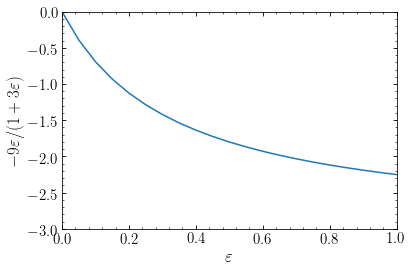
Using that we have assumed that \(r(M) \propto r_\mathrm{max}(M)\) and that in an Einstein–de Sitter Universe \(r_\mathrm{max} \propto r_i/\delta_i \propto M^{\varepsilon+1/3}\) from Equation \(\eqref{eq-spher-collapse-rioverrmax}\), we find that

\begin{equation} \langle \rho \rangle(r) \propto r^{-\frac{9\varepsilon}{1+3\varepsilon}}\,. \end{equation}

Realistic initial peak structures have \(0 < \varepsilon < 1\), giving a power-law density profile with an index \(\gamma\) between \(0\) and \(-9/4\):

figsize(6,4)
eps= numpy.linspace(0.,1.,21)
bovy_plot.bovy_plot(eps,-9*eps/(1.+3*eps),
                    yrange=[-3.,0.],
                    xlabel=r'$\varepsilon$',
                    ylabel=r'$-9\varepsilon/(1+3\varepsilon)$');

The assumptions made about the final apocenter radius of each mass shell and the mass contained within it are, however, violated in more sophisticated modeling. Better models consider spherical, self-similar solutions with radial orbits (Fillmore & Goldreich 1984; Bertschinger 1985) and find that the above formula is incorrect when it predicts \(\gamma > -2\) and the correct power-law is simply \(\gamma = -2\):

figsize(6,4)
eps= numpy.linspace(0.,1.,21)
line_gunngott= bovy_plot.bovy_plot(eps,-9*eps/(1.+3*eps),
                                   yrange=[-3.,0.],
                                   xlabel=r'$\varepsilon$',
                                   ylabel=r'$\gamma$',
                                   label=r'$\mathrm{Gunn\,\&\,Gott}$')
line_selfsim= bovy_plot.bovy_plot(eps,
                                  [-2 if g > -2 else g for g in -9*eps/(1.+3*eps)],
                                  yrange=[-3.,0.],
                                  overplot=True,
                                  label=r'$\mathrm{Self\!-\!similar}$')
legend(handles=[line_gunngott[0],line_selfsim[0]],
       fontsize=18.,loc='upper right',frameon=False);

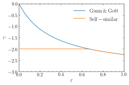
Thus, for purely radial collapse, the equilibrium density profile is \(\rho(r) \approx r^{-2}\), the density profile of an isothermal sphere, which gives a flat rotation curve (see Chapter 6.6.2). When introducing angular momentum and, thus, tangential orbits, solutions can again becomes shallower \((\gamma > -2\)), in particular, isotropized orbit distributions appear to lead to \(\gamma \approx -1\), which is the density profile observed in the inner parts of dark-matter halos in numerical simulations.

In the end, the processes that set the internatl structure of collapsed dark-matter halos are so complex that they need to be studied with numerical \(N\)-body simulations. These studies demonstrate that the density within a dark-matter halo is \(\rho(r) \approx r^{-1}\) near the center, \(\rho(r) \approx r^{-2}\) at intermediate radii, and \(\rho(r) \approx r^{-3}\) as one approaches the virial radius. This is the so-called NFW profile, discussed in more detail in Chapter 3.4.6.

18.3. Collisionless relaxation

\label{sec-dmhaloform-collisionlessrelax}

The formation of virialized dark-matter halos from dynamically-cold initial conditions is a complex process that needs to be studied numerically. Of particular interest is the question of how relaxed, quasi-equilibrium systems form through the effects of self-gravity. In Chapter 6.1, we saw the gravitational dynamics of galactic systems is collisionless—collisions between individual bodies play no role in its evolution—and that the distribution function therefore satisfies the collisionless Boltzmann equation. In Chapter 6.3 we demonstrated that this implies Liouville’s theorem: the phase-space density is conserved along orbital trajectories. “Relaxation” in the thermodynamical sense therefore cannot happen: The six-dimensional phase-space distribution function does not change and there can therefore be no loss of information or increase of entropy associated with its evolution.

The conservation of the phase-space distribution function holds only on a microscopic level, however, not on the macroscopic, observable level. The evolution of a gravitational system causes the phase-space distribution to wrap up in complicated ways, and when averaged—or “coarse-grained”—over a macroscopic volume of phase-space, the distribution function will typically appear to have decreased. On the macroscopic level, systems therefore will appear to approach a relaxed state, even though they are no more relaxed than they were initially at the microscopic level. This type of relaxation that is due to the coarse-grained distribution function evolving while the microscopic one remains constant is called collisionless relaxation.

In the following subsections we discuss a few different types of collisionless relaxation processes that occur during dark-matter halo formation and galaxy evolution. The combination of all of these is what drives an initial dark-matter overdensity to become a virialized halo.

18.3.1. Phase mixing

Phase mixing is perhaps the most important collisionless relaxation process that occurs in galaxies, because it is involved in creating the initial virialized dark-matter halo, but is also instrumental every time a a dark matter halo or a galactic component is perturbed out of its quasi-equilibrium state (e.g., by a minor merger) in driving the system back to quasi-equilibrium.

Phase mixing refers to the process of driving the “phases” of a set of bodies to a uniform distribution, where the “phases” refers to the time-dependent component of an orbit. For example, in the epicycle approximation of orbits in galactic disks that we discussed in Chapter 10.3.1, an orbit consists of three sinusoidal oscillation: the sinusoidal rotation of the guiding center around galactic center, the oscillation around the epicycle, and a vertical oscillation around the galactic mid-plane. Each oscillation has an associated amplitude that is conserved and an associated phase angle that increases linearly in time. More generally, all regular orbits in a galaxy can be described in action-angle coordinates (see Chapter 4.4.3), where the actions are three integrals of motion and the angles are three phase angles that increase linearly in time according to three frequencies. Phase mixing occurs when the phases of a set of orbits that are initially clustered around a given phase become uniform.

Phase mixing happens because the frequencies of nearby points in phase-space generally differ and after long periods of time, the points therefore find themselves at very different phases, even if they started out close together. On a microscopic level, the distribution of phases remains as featured as it was in the initial state—no information is lost during the evolution of regular orbits—but on a macroscopic level the pases will appear to become more uniform. As the phases become uniform, the system will appear to become time-independent, because time dependence for regular orbits can only come from the evolution of the phase distribution, which ceases once it is uniform. Phase mixing therefore drives galactic systems to a quasi-equilibrium state.

As an example, we consider the evolution of a disk of initial conditions in a one dimensional system clustered around an initial \((x,v)\). First we compute the evolution of the phase-space volume of this disk:

from galpy.orbit import Orbit
from galpy.potential import LogarithmicHaloPotential
from galpy.util import bovy_plot
from matplotlib import pyplot
from matplotlib.patches import Polygon
from matplotlib.collections import PatchCollection
# Simple one-dimensional potential
lp= LogarithmicHaloPotential(normalize=1.).toVertical(1.)
# Trace out initially circular phase-space area (in x = 2v)
npoints= 1001
theta= numpy.linspace(0,2.*numpy.pi,npoints,endpoint=True)
phase_space_radius= 0.25
xs= phase_space_radius*2.*numpy.cos(theta)+1.
vs= phase_space_radius*1.*numpy.sin(theta)+1
# Integrate all points along the edge of the area
os= [Orbit([x,v]) for x,v in zip(xs,vs)]
nts= 1001
ts= numpy.linspace(0.,120.5,nts)
[o.integrate(ts,lp) for o in os]
ts= [0,10,40,120]
# Plot
bovy_plot.bovy_print(axes_labelsize=17.,text_fontsize=12.,
                     xtick_labelsize=15.,ytick_labelsize=15.)
figsize(10,10)
fig, axes= pyplot.subplots(2,2)
axes= axes.flatten()
for ii,(ax,t) in enumerate(zip(axes,ts)):
    # Create matplotlib polygons to represent area at each time
    polygon= Polygon(numpy.array([[o.x(t),o.vx(t)] for o in os]),
                     closed=True)
    p= PatchCollection([polygon],alpha=1.)
    sca(ax)
    ax.add_collection(p)
    xlim(-3.5,3.5)
    ylim(-1.75,1.75)
    xlabel(r'$x$')
    ylabel(r'$v$')
    ax.tick_params(labelbottom=False,labelleft=False)
    bovy_plot.bovy_text(r'$t={:d}$'.format(t),top_left=True,size=18.);

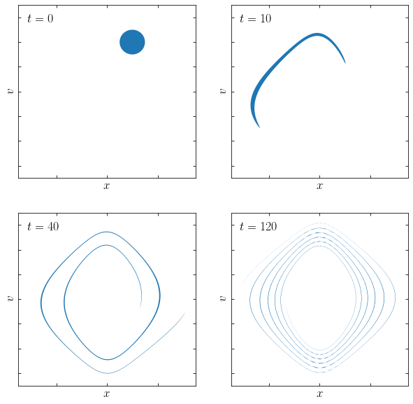
Because the frequencies of different orbits present in the initial disk differ, the disk quickly starts to spread. Eventually the disk turns into a thin ribbon that wraps around the center many times. Because the microscopic phase-space volume is conserved, the total area of the ribbon is the same as the area of the inital disk, but now spread over a much wider area of phase-space. If we coarse-grain the distribution function, the area of the region covered by the ribbon would be larger and the distribution function would therefore be lower. To illustrate that phase-mixing happens in this system at the coarse-grained level, we instead sample points uniformly within the initial disk and integrate their orbits. In the following figure we plot their phase-space positions at the same times as above, showing individual points with large symbols to perform a visual coarse-graining:

# Simple one-dimensional potential
lp= LogarithmicHaloPotential(normalize=1.).toVertical(1.)
# sample points within initially circular phase-space area (in x = 2v)
npoints= 3001
theta= numpy.random.uniform(size=npoints)*2.*numpy.pi
phase_space_radius= 0.25*numpy.sqrt(numpy.random.uniform(size=npoints))
xs= phase_space_radius*2.*numpy.cos(theta)+1.
vs= phase_space_radius*1.*numpy.sin(theta)+1
# Integrate all points
os= [Orbit([x,v]) for x,v in zip(xs,vs)]
nts= 1001
ts= numpy.linspace(0.,120.5,nts)
[o.integrate(ts,lp) for o in os]
ts= [0,10,40,120]
# Plot
bovy_plot.bovy_print(axes_labelsize=17.,text_fontsize=12.,
                     xtick_labelsize=15.,ytick_labelsize=15.)
figsize(10,10)
fig, axes= pyplot.subplots(2,2)
axes= axes.flatten()
for ii,(ax,t) in enumerate(zip(axes,ts)):
    sca(ax)
    ax.plot([o.x(t) for o in os],[o.vx(t) for o in os],
            'o',alpha=0.3,ms=10,mec='none')
    xlim(-3.5,3.5)
    ylim(-1.75,1.75)
    xlabel(r'$x$')
    ylabel(r'$v$')
    ax.tick_params(labelbottom=False,labelleft=False)
    bovy_plot.bovy_text(r'$t={:d}$'.format(t),top_left=True,size=18.);

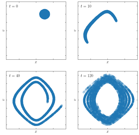
It is clear that at the final time, the distribution of the points appears to uniformly occupy the part of phase-space allowed by the initial energies. The phase-space distribution is therefore phase-mixed.

Phase mixing occurs in all non-uniform mass density distributions (we showed in Chapter 5.2.1 that the frequencies of all orbits in a uniform density sphere are all commensurate, but this is not the case in any other mass distribution). The timescale of phase-mixing depends on the initial frequency distribution as \(\tau \approx 2\pi/\Delta \Omega\), where \(\Delta \Omega\) is the typical spread in the initial frequencies. If the initial distribution has \(\mathcal{O}(1)\) frequency differences, phase-mixing occurs on a dynamical time, because \(\tau \approx 2\pi/\Delta \Omega \approx 2\pi/\Omega = t_\mathrm{dyn}\). If the frequency distribution is narrow—or “colder”—the phase-mixing timescale is longer and can be many Gyr for very cold systems (for example, globular cluster streams phase-mixing into the halo of the Milky Way have \(\Omega / \Delta \Omega \approx 100\), so \(\tau \approx 100\,t_\mathrm{dyn}\)).

18.3.2. Violent relaxation

Phase mixing is a relatively benign process that happens predictably, at a steady rate, and within both evolving or static mass distributions. Because phase mixing only changes the phases of the orbits, but not their integrals of motion like the energy, it leads to only small changes to the global structure of a system. In static systems, the three integrals of the motion—the actions in action-angle coordinates—are conserved for regular orbits and the only way mix the integrals of the motion themselves is therefore to have a time-dependent gravitational potential.

An initially-collapsing dark-matter halo has a strongly time-variable gravitational potential after shell crossing and the energies and other quantities that would be conserved in a static potential can therefore evolve. Lynden-Bell (1967) termed this process violent relaxation, because, as he argued, it occurs on a dynamical time and is therefore fast compared to other collisionless relaxation processes (and certainly compared to collisional relaxation for galactic systems, which has \(\tau \approx N\,t_\mathrm{dyn}\)). Violent relaxation causes the energies of individual bodies to change and in general leads to a broadening of the energy distribution. A broadening of the energy distribution leads to a broadening of the distribution of orbital frequencies and phase-mixing therefore also becomes more rapid, leading to a relaxed phase-mixed state.

Violent relaxation is a self-limiting process. Violent relaxation requires a time-dependent potential to operate, but drives systems towards a quasi-equilibrium state in which the potential no longer changes in time and violent relaxation therefore ceases. Simulations of the formation of dark-matter halos show that violent relaxation occurs, but is never complete, in the sense that the final energy of particles are correlated with their initial energy. The system therefore retains some memory of its initial condition and violent relaxation does not lead to any sort of thermodynamic steady state.