
11. Equilibria of galactic disks
In Chapter 8, we discussed how to compute the gravitational potential and the gravitational field of a general disk mass distribution. In Chapter 9, we used the kinematics of tracers on circular orbits or nearly-circular orbits to learn about the mass distributions of disk galaxies. This led to the important conclusion that we require large quantities of dark matter to explain the kinematics of galactic rotation in disk galaxies. In this chapter, we will go beyond circular or nearly-circular orbits in disk galaxies and we will investigate the dynamical equilibrium distribution of stars in disk galaxies, assuming axisymmetry as in the previous chapters. This will allow us to understand the galactic rotation of stars in the solar neighborhood, including older stars that have orbits that deviate significantly from circular rotation. We will also discuss the dynamical equilibrium state of stars in the direction perpendicular to the disk plane, a dimension which is similarly absent in the circular-rotation approximation of Chapter 9 that assumes that all bodies orbit in the disk’s mid-plane. The framework that we will develop will also let us constrain the presence of dark matter at the Sun’s position, which is difficult to do from the rotation curve alone. This is because stars and gas dominate the radial force that sets the local circular velocity and it is difficult to unambiguously determine the local dark-matter density from the Milky Way’s circular velocity curve near the Sun alone.
We will investigate the properties of the equilibrium states of axisymmetric galactic disks using the same general tools that we first introduced in Chapter 6: the Jeans equations (Chapter 6.4) to connect the density profile to the first and second moments of the kinematics (mean velocities and velocity dispersions) and the Jeans theorem (Chapter 6.5) to build full phase-space distribution functions of galactic disks. While the Jeans equations generalize to a slightly more complicated form in the axisymmetric case than the spherical Jeans equations of Chapter 6.4.2, we will see that building phase-space models using the Jeans theorem is significantly more complicated than it was in the spherical case.
The Jeans theorem tells us that equilibrium phase-space models of galactic disks are functions of the integrals of motion. As shown in Chapter 10.1, orbits in a static, axisymmetric gravitational potential have two classical integrals of motion: the specific energy \(E\) and the component of the specific angular momentum parallel to the symmetry axis (conventionally the \(z\) axis, \(L_z\)). However, we also saw in Chapter 10.2 that these orbits typically appear to conserve a third, non-classical integral (we will discuss this in more detail in Chapter 14). While we may be tempted to ignore this third integral and work with equilibrium models \(f \equiv f(E,L_z)\), a simple observation about the kinematics of stars in galactic disks demonstrates that this cannot produce realistic models: the vertical velocity dispersion \(\sigma_z\) of stars near the Sun is typically about half of the radial velocity dispersion \(\sigma_R\) (in cylindrical coordinates; e.g., Wielen 1974; Mackereth et al. 2019), varying between \(\approx0.4\) to \(\approx0.6\) depending on the age and angular momentum of the star. The same holds in external galaxies (Bottema 1993). If the distribution function only depends on \(E\) and \(L_z\), however, these dispersions should be equal to each other, because the vertical and radial velocity only appear in \(E\) and they do so in the same way (in the combination \(v_R^2/2+v_z^2/2\)). Thus, the phase-space distribution of stars near the Sun must depend on a third integral that, at a given \(E\) and \(L_z\) distinguishes between stars with greater or smaller vertical oscillations. The third integral is typically denoted as \(I_3\) and the distribution function therefore has to be \(f \equiv f(E,L_z,I_3)\).
For most realistic galactic potentials, we cannot write down an expression for the third integral and this makes the task of writing down equilibrium disk models \(f(E,L_z,I_3)\) challenging. To make headway in this chapter, we will follow two related approaches. First, we will describe equilibrium models for axisymmetric, razor-thin disks. Defining \(I_3\) such that \(I_3 = 0\) describes an orbit with zero vertical oscillation, such models have \(f(E,L_z,I_3) = f(E,L_z)\,\delta(I_3)\) (using somewhat sloppy notation, we use the same ‘\(f\)’ here for the three- and two-integral distribution function). Because these models are only non-zero within the mid-plane and/or for zero velocity perpendicular to the mid-plane, we do not need to be able to compute the third integral. Of course, we can only use these models to learn about the dynamical state within the mid-plane, not that perpendicular to it, but we will see that they are nevertheless useful for describing stars in the Milky Way.
To add a non-zero vertical extension to these models, we will make use of the insights about the basic properties of orbits in disk mass distributions in Chapter 10. There we looked at orbits with relatively high angular momenta, which are on disk orbits that are close to circular but not necessarily “nearly” circular (which we define here as so close to circular that the epicycle approximation provides a very good description of their orbits). We demonstrated that for such orbits the motion in the disk plane approximately separates from the motion perpendicular to the disk plane. We can usefully decompose orbits in the disk into their planar component and their vertical component (at the mean radius of the orbit) and still understand the basic orbital properties, such as the closest and furthest cylindrical radii \(R\) reached within the plane and the maximum height \(|z|\) above the plane. Because all of the orbits approximately separate in planar and vertical components, the distribution of orbits can also be approximately separated into planar and vertical components, with little coupling between the two. As discussed in Chapter 10.2, we can split the Hamiltonian into a planar and vertical part and radial \(E_R\) and vertical \(E_z\) contributions to the energy are separately conserved: \(E_R = v_R^2/2+v_\phi^2/2+\phi(R,z=0)\) and \(E_z = v_z^2/2+\Phi(R,z)-\Phi(R,z=0)\). We can then identify the third integral as \(I_3 = E_z\) and build models using this third integral. A simple way to do this is to combine the functional form of razor-thin models, \(g(E,L_z)\), that we will discuss first in this chapter, with the functional form of one-dimensional models \(h(E_z)\) for the dynamics perpendicular to the mid-plane that we will discuss in Section 11.4. By allowing the parameters of \(h\) to depend on the guiding-center radius through \(L_z\), we can arrive at three-dimensional distribution functions \(f(E,L_z,E_z) = g(E,L_z)\times h(E_z;L_z)\) that accurately describe the dynamics in the plane and the radially-dependent dynamics perpendicular to the plane (e.g., Kuijken & Dubinski 1995).
11.1. The axisymmetric Jeans equations and the asymmetric drift
Similar to what we did for spherical systems in Chapter 6.4, to start exploring the steady-state dynamics of galactic disks, we first consider moments of the collisionless Boltzmann equation and construct the cylindrical Jeans equations for axisymmetric systems.
11.1.1. The axisymmetric Jeans equations
To derive the cylindrical Jeans equations, we start from the equilibrium collisionless Boltzmann Equation (6.36) for the distribution function \(f\). We write this equation in cylindrical coordinates by using the Hamiltonian in cylindrical coordinates, which is (see Equation 4.59)
where we have as usual set \(m=1\) and the momenta are given in terms of the velocity as
The equilibrium collisionless Boltzmann equation is then
For an axisymmetric system in an axisymmetric potential, the derivatives of \(f\) and \(\Phi\) with respect to \(\phi\) vanish and this equation simplifies to
Multiplying this equation by \(p_R\) and integrating over the three components of the momentum \((p_R,p_\phi,p_z)\) using that \(\mathrm{d} p_R\,\mathrm{d} p_\phi\,\mathrm{d}p_z = R\,\mathrm{d}v_R\,\mathrm{d} v_\phi\,\mathrm{d}v_z\) (where \(v_\phi = R\,\dot{\phi}\)) and using partial integration to deal with the partial derivative with respect to \(p_R\), this becomes
or
This is the axisymmetric, radial Jeans equation. If we instead multiply Equation \(\eqref{eq-collisionless-boltzmann-equil-cyl}\) by \(p_z\) and integrate over all of the momenta, we obtain
which is the axisymmetric, vertical Jeans equation. Multiplying Equation \(\eqref{eq-collisionless-boltzmann-equil-cyl}\) by \(p_\phi\) produces a Jeans equation that relates \(\overline{v_R\,v_\phi}\) and \(\overline{v_z\,v_\phi}\), both of which are zero if the distribution function is a function of the energy \(E\) and \(L_z\) alone.
As discussed at the beginning of this chapter, in Chapter 10.2, we demonstrated that for orbits that do not travel to large heights above and below the mid-plane of a disk mass distribution, the motion in the radial direction approximately decouples from that in the vertical direction, in which case the Hamiltonian can be approximately written as \(H = H_{R,\mathrm{eff}}(R,p_R) + H_z(z,p_z)\), and three integrals of the motion can be chosen to be \((L_z,E_R,E_z)\), where \(E_R\) and \(E_z\) are the energies corresponding to the planar and vertical components of the motion. From a stronger version of the Jeans theorem (which we did not discuss) it follows that the steady-state distribution function can only depend on these three integrals \((L_z,E_R,E_z)\), which in turn are only functions of the following combinations of the velocities: \(v_\phi\) (from \(L_z\)), \(v_R^2\) (from \(E_R\)), and \(v_z^2\) (from \(E_z\)). Therefore we have that in the separable limit, \(\overline{v_R^2} = \sigma_R^2\), \(\overline{v_z^2} = \sigma_z^2\), \(\overline{v_R\,v_z} = 0\), and \(\overline{v_\phi^2} = \overline{v_\phi}^2+\sigma_\phi^2\). The axisymmetric Jeans equations then simplify to
Because the distribution of stellar orbits approximately decouples to a much better level than individual orbits do, these equations approximately hold for most of the stars in the solar neighborhood (roughly those that reach maximum \(|z| \lesssim1\,\mathrm{kpc}\)).
11.1.2. The asymmetric drift
Returning to the general case of the radial Jeans equation in Equation \(\eqref{eq-jeans-radial-axi}\), we write \(\overline{v_\phi^2} = \overline{v_\phi}^2+\sigma_\phi^2\) and evaluate the equation at \(z=0\), where \(\partial \Phi / \partial R = v_c^2(R)/R\). This can be written as
Under the assumption that \(\partial \nu / \partial z = 0\) (good for a symmetric stellar distribution around the mid-plane that smoothly turns over at \(z=0\)), we can also write this as
For stars that are on close-to-circular orbits, \(\overline{v_R^2} \ll v_c^2\) and thus \(v_c-\overline{v_\phi} \ll v_c\) from this equation (the part in square brackets is a number of order one). Then we can approximate \(v_c+\overline{v_\phi} \approx 2\,v_c\), which gives the Stromberg asymmetric drift equation
This equation demonstrates that for stars that are on close-to-circular orbits, the difference between the circular velocity \(v_c\) and the mean rotational velocity \(\overline{v_\phi}\) is proportional to the radial velocity dispersion (\(\sigma_R^2 \approx \overline{v_R^2}\) for any reasonable disk distribution function). In particular, Equation \(\eqref{eq-stromberg}\) shows that the mean rotational velocity is not necessarily equal to \(v_c\) when \(\overline{v_R^2} > 0\).
To get a better sense of what Equation \(\eqref{eq-stromberg}\) implies, we can use further approximations that are appropriate for nearly-circular orbits. For such orbits the radial and vertical motion decouples and \(\overline{v_R\,v_z} \approx 0\), as discussed above, and \(\overline{v_R^2} = \sigma_R^2\). In Chapter 10.3.2, we derived the relation \(\sigma_\phi^2 / \sigma_R^2 = B/(B-A)\), where \(A\) and \(B\) are the Oort constants. Furthermore, for typical disk populations (although not all), both \(\nu\) and \(\sigma_R^2\) decrease with increasing \(R\) and we can approximate each as having an exponential dependence: \(\nu(R) \approx e^{-R/h_R}\) and \(\sigma_R^2 \approx e^{-R/h_{2\sigma_R}}\); therefore \(\partial \ln [\nu\,\overline{v_R^2}]/\partial \ln R = -R\,(1/h_R+1/h_{2\sigma_R})\). Using all of these approximations, Equation \(\eqref{eq-stromberg}\) becomes
When looking at a sample of stars near the Sun, the second term in the square brackets in this equation is typically positive (but not always) and is larger than the first term is negative: for a flat rotation curve, \(A/(B-A) = -0.5\) and the Sun’s distance from the center \(R_0\) is typically larger than \(h_R/2\), such that the quantity in the square bracket is positive. The difference \(v_c-\overline{v_\phi}\) is then positive and the mean rotational velocity is less than the circular velocity. This is a first manifestation of the general phenomenon of asymmetric drift in disk galaxies: the distribution of rotational velocities at a given point in a disk galaxy is asymmetric around \(v_\phi = v_c(R)\) and therefore the mean rotational velocity is different from the circular velocity. Later in this chapter, we will see that the distribution of \(v_\phi\) is also skewed, not just simply shifted to a different mean. This phenomenon makes it difficult to relate the observed rotational velocity of a set of stars to the circular velocity: in the previous chapter we assumed that gas is on circular orbits such that its observed velocity directly tells us about the circular velocity; for stars we cannot simply generalize this to use the mean observed velocity without taking into account the asymmetric drift.
We will look the Stromberg asymmetric drift equation in the context of the solar neighborhood further in Section 11.3.2 below.
11.2. Distribution functions for razor-thin disks
Now that we have discussed the Jeans equations that relate the moments of steady-state distribution functions for disks, we present some examples of full steady-state distribution functions in this section. Again, because to a good approximation we can consider the planar part of a star’s orbit in a disk mass distribution as being decoupled from the vertical motion, we start by describing distribution functions for razor-thin disks. These distribution functions are all functions \(f(E,L_z)\) of the planar part of the energy, which we will simply write as \(E\) here, and the \(z\) component of the angular momentum \(L_z\). As discussed at the beginning of this chapter, there is an implied multiplication of \(f(E,L_z)\) with \(\delta(I_3)\) that we will not carry around, but that causes the distribution function to be zero for any non-zero \((z,v_z)\). Because the distribution function is zero for non-zero \((z,v_z)\), we will simply work in the mid-plane in this section and drop the vertical dependence of any quantity, e.g., the potential will be \(\Phi(R) \equiv \Phi(R,z=0)\).
When we discussed steady-state distribution functions for spherical systems we spend much time on self-consistent models where the gravitational potential is sourced by the density obtained by integrating the distribution function over velocity—that is, the distribution function’s implied density satisfies the Poisson equation with the total gravitational potential. As we saw in Chapter 9, galactic disks are embedded in massive dark-matter halos and at any point in the disk a significant fraction of the gravitational force is contributed by the dark matter. Moreover, stellar disks like the Milky Way are made up of an almost continuous sequence of stellar populations (e.g., of different ages) that taken together generate the gravitational potential of the stellar disk. We will find it much easier to create distribution function models for simpler components of the full stellar disk (e.g., a single age population) than for the full stellar disk at once. Thus, when dealing with disks, self-consistency is not as important a consideration when discussing steady-state disk distribution functions and most of the models that we will discuss are not self-consistent. In particular, in most examples below, we will write down equilibrium disk models for exponential disks embedded in a gravitational potential with a flat rotation curve, which as we know from Chapter 8.3.3.2 is not a self-consistent setup, but it is a realistic description of the dynamics of stellar disks.
11.2.1. The distribution function of a cold, rotating disk
We now turn to the question of how we can determine a razor-thin distribution function for a rotating disk with a given surface density \(\Sigma(R)\) in a given axisymmetric potential \(\Phi(R)\), which is not self-consistently generated by \(\Sigma(R)\). We start by building a disk distribution function for a cold disk with zero velocity dispersion and then warm it up by introducing non-zero velocity dispersion in Section 11.2.2 below. These distribution functions are all functions of the energy \(E\) and \(z\)-component of the angular momentum \(L_z\). The derivation in this and the next section follows that of Dehnen (1999).
From the Stromberg asymmetric drift Equation \(\eqref{eq-stromberg}\) it is clear that an axisymmetric disk with vanishing velocity dispersion \(\overline{v_R^2} = 0\) must be rotating at the circular velocity at each radius. Thus, we can build the full disk out of circular orbits and the form of the distribution function must be
where \(E_c[L_z]\) is the energy of a circular orbit with angular momentum \(L_z\) and \(F(L_z)\) is a function that we need to determine from the condition that this distribution function corresponds to a given surface density \(\Sigma(R)\). Because we only need to consider orbits that are infinitesimally close to a circular orbit in this distribution function, we can work out the energy in the epicycle approximation. The energy difference in the epicycle approximation is given by
where \(X\) is the amplitude of the epicyclic motion and \(\alpha\) is the phase (see Equations 10.16 and 10.28). In Chapter 10.3.2 we demonstrated that \(v_\phi - v_c = -2B\,X\,\cos(\kappa t + \alpha)\) where \(v_c\) is the circular velocity at \(R\) (up to terms that are second order in \(X\); Equation 10.44). substituting that \(-4B = \kappa^2/\Omega\), we can therefore also write the energy difference as
where we have substituted \(\gamma = 2\Omega/\kappa\). Thus, we can write the distribution function in Equation \(\eqref{eq-cold-df-form}\) in terms of \((R,\phi,v_R,v_\phi)\) as
The factor of two accounts for the \(E < E_c[L_z]\) part of the distribution function which we have dropped when going to the epicycle approximation (this is necessary to keep the delta function properly normalized). The surface density corresponding to this distribution function is
In this calculation, we introduced polar velocity coordinates \((v,\psi)\) with \(v_R = v\,\cos\psi\) and \(\tilde{v}_\phi = v\sin \psi\) to perform the integral over the delta function and we used that \(\int_0^\infty \mathrm{d}x\,f(x)\,\delta(x) = f(0)/2\) (Equation B.8). For \(\Sigma'(R)\) to equal \(\Sigma(R)\), we therefore need to choose the function \(F(L_z)\) as
where \(R_L = R_g(L_z)\) is the guiding-center radius of a circular orbit with angular momentum \(L_z\) (see Equation 10.13; while we generally denote the guiding-center radius as \(R_g\), here we use \(R_L\) to clearly distinguish the radius definition’s dependence on \(L_z\) from an alternative radius definition in terms of \(E\) in the Dehnen distribution function below, where we will denote the equivalent radius as \(R_E\)). Note that in this expression, \(\gamma\) in general also depends on \(R_L\). The distribution function for a cold disk with surface density \(\Sigma(R)\) is therefore
11.2.2. Distribution functions for warm, rotating disks
Now that we have derived a general expression for the distribution function of a cold, rotating disk, we ask how we can generalize it to have a given velocity dispersion profile \(\sigma_R(R)\). For a distribution function that depends on \((E,L_z)\) there is no unique solution to this problem. Just like in the spherical case, the Jeans equations do not close even if we derive higher and higher-order versions of it. Specifying \(\Sigma(R)\) and \(\sigma_R(R)\) still leaves freedom in the higher-order moments of the velocity distribution that is not fixed by the assumption of a steady state. To model the distribution function of a population of stars in a disk, we therefore need to use additional assumptions about their velocity distribution to specify a unique model.
Below we discuss three examples of how to generalize the cold disk distribution function in Equation \(\eqref{eq-colddisk-df}\). All three of these examples generalize the expression by replacing the delta function by a function \(K[\cdot]\) that has a finite width \(\sigma_R^2(R)\): \(\delta(E-E_c[L_z]) \rightarrow K[(E-E_c[L_z])/\sigma_R^2(R)]\): whereas for the cold distribution function, the only populated orbits at a given angular momentum \(L_z\) are the circular orbits with \(E = E_c[L_z]\), in these warm distribution functions, orbits at a given \(L_z\) are populated according to \(K[(E-E_c[L_z])/\sigma_R^2(R)]\). This general approach of creating warm disk distribution functions by warming up the cold distribution function is the main way in which even more complex and realistic disk distribution functions than we discuss in this chapter are obtained (e.g. Binney 2010; Binney & McMillan 2011).
From the derivation of the cold-disk distribution function, it should be clear that simply replacing the delta function with a finite-width kernel \(K[\cdot]\) will not produce \(\Sigma'(R) = \Sigma(R)\) using the prefactor in Equation \(\eqref{eq-colddisk-F}\): the derivation of this prefactor depends on the kernel being a delta function, and only if both \(\Sigma(R)\) and \(\sigma_R(R)\) are independent of \(R\) would \(\Sigma'(R) = \Sigma(R)\). Similarly, if we compute the actual velocity dispersion \(\sigma'_R(R)\) in the radial direction as the square root of the second moment in \(v_R\) of the distribution function, we find that \(\sigma'_R \neq \sigma_R\). We therefore have to either (i) derive a new prefactor \(F(L_z)\) such that \(\Sigma'(R) = \Sigma(R)\) or (ii) live with the fact that we only have \(\Sigma'(R) \approx \Sigma(R)\) without having exact equality between the two. We will largely take path (ii) here and not worry too much about the exact equality the “target” \(\Sigma(R)\) and \(\sigma_R(R)\) and the distribution function’s actual \(\Sigma'(R)\) and \(\sigma'_R(R)\).
11.2.2.1. The Schwarschild distribution function
The first and simplest example of a warmed-up disk distribution function replaces the delta function in Equation \(\eqref{eq-colddisk-df}\) with an exponential function
where \(\sigma_R(R)\) is a function that controls the velocity dispersion and the exponential is normalized such that integrating it from \(E=E_c[L_z]\) to \(E=\infty\) equals one. The Schwarzschild distribution function results from approximating the argument of the exponential using the epicycle approximation in Equation \(\eqref{eq-EEc-epicycle}\)
This is a distribution function that is only approximately in a steady state, because the energy difference \(E-E_c[L_z]\) is only equal to \([v_R^2 + \gamma^2\,(v_\phi - v_c)^2]/2\) for nearly circular orbits. The surface density \(\Sigma'(R)\) corresponding to the Schwarzwchild distribution function is
Because of the \(R_L\) dependence of \(\sigma_R\) in the integrand, for general \(\sigma_R(R)\) this integral needs to be calculated numerically. However, when \(\sigma_R/v_c \ll 1\) then we can treat all functions that depend on \(R_L\) as being constant over the range where the integrand is significantly non-zero and we find that \(\Sigma'(R) = \Sigma(R)\). Thus, for \(\sigma_R/v_c \ll 1\) where only close-to-circular orbits are populated significantly, we have that \(\Sigma'(R)\approx\Sigma(R)\).
Following a similar argument we have that for close-to-circular orbits \(\overline{v_\phi} \approx v_c(R)\), \(\sigma'_R(R) \approx \sigma_R(R)\), and \(\sigma'_\phi(R) \approx \sigma'_R(R)/\gamma\) (in agreement with \(\sigma'_\phi(R)/\sigma'_R(R) = \sqrt{B/(B-A)}\) in the epicycle approximation). In fact, the entire velocity distribution implied by the Schwarzschild distribution function for \(\sigma_R/v_c \ll 1\) is nearly Gaussian. When the velocity dispersion \(\sigma_R(R)\) is larger, the \(R_L = L_z/v_c\) dependence of the \(\Sigma\), \(\gamma\), and \(\sigma_R\) functions in the distribution function cause the distribution to no longer be Gaussian.
As an example of the Schwarzschild distribution function, we consider the family defined by
for different values of the velocity dispersion parameter \(\sigma_0\) at \(R=1\). That is, both the surface density profile \(\Sigma(R)\) and the velocity-dispersion profile \(\sigma_R(R)\) are exponential, the former with a scale length of \(1/3\) and the latter with a scale length of \(1\) (this is a not-unreasonable model for stars near the Sun). As the background potential, we use a potential with a flat rotation curve: \(\Phi(R) = v_c^2\,\ln R\) in the plane. First we numerically compute \(\Sigma'(R)\) and compare it to \(\Sigma(R)\) for a model with a relatively high \(\sigma_0/v_c = 0.15\) and we do the same for \(\sigma'_R(R)\), comparing it to \(\sigma_R(R)\):
[4]:
from galpy.df import schwarzschilddf
df_warm= schwarzschilddf(profileParams=(1./3.,1.0,0.15),beta=0.)
Rs= numpy.linspace(0.1,2.,101)
figsize(10,4)
subplot(1,2,1)
sigmaprime= numpy.array([df_warm.surfacemass(R) for R in Rs])
line_sprime= semilogy(Rs,sigmaprime,zorder=1,
                     label=r"$\Sigma'(R)$")
sigma= numpy.array([df_warm.targetSurfacemass(R) for R in Rs])
line_sdens= semilogy(Rs,sigma,zorder=0,
                    label=r"$\Sigma(R)$")
xlabel(r'$R$')
xlim(0.,2.3)
legend(handles=[line_sprime[0],line_sdens[0]],
       fontsize=18.,loc='upper right',frameon=False)
subplot(1,2,2)
sigma2prime= numpy.array([df_warm.sigma2(R) for R in Rs])
line_sprime= plot(Rs,numpy.sqrt(sigma2prime),zorder=1,
                     label=r"$\sigma_R'(R)/v_c$")
sigma2= numpy.array([df_warm.targetSigma2(R) for R in Rs])
line_sigma2= plot(Rs,numpy.sqrt(sigma2),zorder=0,
                    label=r"$\sigma_R(R)/v_c$")
xlabel(r'$R$')
xlim(0.,2.3)
ylim(0.,0.4)
legend(handles=[line_sprime[0],line_sigma2[0]],
       fontsize=18.,loc='upper right',frameon=False);
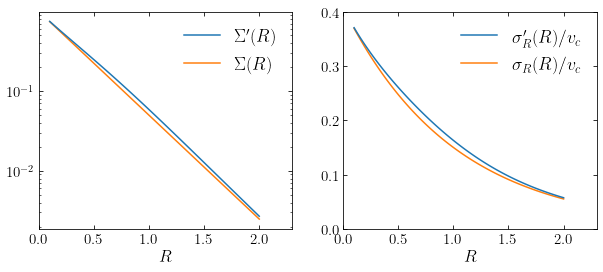
We see that \(\Sigma'(R)\) is indeed approximately equal to \(\Sigma(R)\). The agreement between \(\sigma'_R(R)\) and \(\sigma_R(R)\) is less good and \(\sigma'_R(R)\) is higher by about 10% than \(\sigma_R(R)\) over much of the range in \(R\). Nevertheless, the overall shape and amplitude of both \(\Sigma'(R)\) and \(\sigma'_R(R)\) are in relatively good agreement with \(\Sigma(R)\) and \(\sigma_R(R)\).
The distribution of azimuthal velocities for different values of \(\sigma_0\) at \(R=1\) is given in the following figure (with arbitrary overall normalization of each distribution):
[18]:
from galpy.df import schwarzschilddf
df_cold= schwarzschilddf(profileParams=(1./3.,1.0,0.02),beta=0.)
df_warmer= schwarzschilddf(profileParams=(1./3.,1.0,0.07),beta=0.)
df_warm= schwarzschilddf(profileParams=(1./3.,1.0,0.15),beta=0.)
vts= numpy.linspace(0.4,1.5,201)
figsize(7.75,4)
ycold= numpy.array([df_cold(numpy.array([1.,0.,vt])) for vt in vts])
line_cold= plot(vts,ycold/(numpy.amax(ycold)+numpy.random.uniform()/10.),
                label=r'$\sigma_0 = 0.02\,v_c$')
ywarmer= numpy.array([df_warmer(numpy.array([1.,0.,vt])) for vt in vts])
line_warmer= plot(vts,ywarmer/(numpy.amax(ywarmer)+numpy.random.uniform()/10.),
                  label=r'$\sigma_0 = 0.07\,v_c$')
ywarm= numpy.array([df_warm(numpy.array([1.,0.,vt])) for vt in vts])
line_warm= plot(vts,ywarm/(numpy.amax(ywarm)+numpy.random.uniform()/10.),
                label=r'$\sigma_0 = 0.15\,v_c$')
xlabel(r'$v_\phi/v_c$')
legend(handles=[line_cold[0],line_warmer[0],line_warm[0]],
       fontsize=18.,loc='upper left',frameon=False);
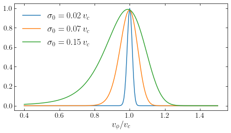
The coldest distribution function has \(\sigma_0/v_c = 0.02\) and therefore consists of stars only on nearly circular orbits. The distribution of azimuthal velocities is strongly peaked at \(v_\phi = v_c\) and the distribution is close to symmetric and Gaussian. When we increase \(\sigma_0/v_c\), we see that the distribution becomes wider, because of the higher velocity dispersion, but also becomes asymmetric. Especially in the case where \(\sigma_0/v_c = 0.15\) the velocity distribution is highly asymmetric. This is another manifestation of the asymmetric drift. The mean azimuthal velocity \(\overline{v_\phi} < v_c\) for these examples, because both \(\Sigma(R)\) and \(\sigma_R(R)\) are declining functions of \(R\) (see Equation \([\ref{eq-stromberg}]\)). Physically what happens is that at a given radius \(R\), stars with \(v_\phi > v_c\) must have guiding-center radii \(R_g > R\), because of the conservation of angular momentum: \(R\,v_\phi = R_g\,v_c\) or \(v_\phi/v_c = R_g/R > 1\) (remember that we are working in a disk with a flat rotation curve, \(v_c = \mathrm{constant}\)). Similarly, stars with \(v_\phi < v_c\) must have \(R_g < R\). Now, because the surface density declines with radius—\(\Sigma(R_g < R) > \Sigma(R_g > R)\)—there are more stars with \(v_\phi < v_c\) at \(R\) than there are stars with \(v_\phi > v_c\) and the average \(\overline{v_\phi} < v_c\). The decline of the velocity dispersion increases this effect: that \(\sigma_R(R_g < R) > \sigma_R(R_g > R)\) means that stars from \(R_g < R\) have \(|R_g-R|\) that is typically larger than \(|R_g-R|\) from stars with \(R_g > R\), and thus, that \(|v_\phi-v_c|\) is larger for stars coming from \(R_g < R\) than it is for stars coming from \(R_g > R\), further pulling the mean \(\overline{v_\phi}\) to smaller values. Thus, there are more stars coming from inner radii and these are typically coming from further inwards than there are stars coming from outer radii, leading to \(\overline{v_\phi} < v_c\) and skewing the \(v_\phi\) distribution.
Lest your take-away from this discussion is that \(\overline{v_\phi} < v_c\) always holds, it is important to keep in mind that it does not have to be the case that \(\overline{v_\phi} < v_c\); the sign of the \(\overline{v_\phi} \neq v_c\) difference is set by the gradient of \(\Sigma'\) and \(\sigma'_R\) (see Equation \([\ref{eq-stromberg}]\)). While the overall stellar distribution in a disk galaxy is decreasing outwards and thus for the disk as a whole we expect \(\overline{v_\phi} < v_c\), sub-populations of stars (e.g., young stars) might have surface density profiles that increase outwards. In that case, the asymmetric drift could work the other way around and produce \(\overline{v_\phi} > v_c\) when measuring \(\overline{v_\phi}\) for that population of stars. As an example, we show the distribution of \(v_\phi\) for the same model as above, but using \(\Sigma(R) = \Sigma_0\,e^{R_0/3}\) (and keeping the slowly declining \(\sigma_R\)):
[17]:
from galpy.df import schwarzschilddf
df_cold= schwarzschilddf(profileParams=(-1./3.,1.0,0.02),beta=0.)
df_warmer= schwarzschilddf(profileParams=(-1./3.,1.0,0.07),beta=0.)
df_warm= schwarzschilddf(profileParams=(-1./3.,1.0,0.15),beta=0.)
vts= numpy.linspace(0.4,1.5,201)
figsize(7.75,4)
ycold= numpy.array([df_cold(numpy.array([1.,0.,vt])) for vt in vts])
line_cold= plot(vts,ycold/(numpy.amax(ycold)+numpy.random.uniform()/10.),
                label=r'$\sigma_0 = 0.02\,v_c$')
ywarmer= numpy.array([df_warmer(numpy.array([1.,0.,vt])) for vt in vts])
line_warmer= plot(vts,ywarmer/(numpy.amax(ywarmer)+numpy.random.uniform()/10.),
                  label=r'$\sigma_0 = 0.07\,v_c$')
ywarm= numpy.array([df_warm(numpy.array([1.,0.,vt])) for vt in vts])
line_warm= plot(vts,ywarm/(numpy.amax(ywarm)+numpy.random.uniform()/10.),
                label=r'$\sigma_0 = 0.15\,v_c$')
xlabel(r'$v_\phi/v_c$')
legend(handles=[line_cold[0],line_warmer[0],line_warm[0]],
       fontsize=18.,loc='upper left',frameon=False);
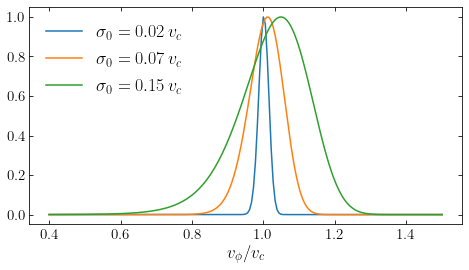
Because the velocity dispersion still decreases with increasing \(R\), there is now a competition between the two effects discussed in the previous paragraph. But on the whole, the surface density wins out and the velocity distribution has a mean \(\overline{v_\phi} > v_c\) in this case. This effect does in fact happen for low-metallicity stars in the solar neighborhood, which have negative asymmetric drifts.
11.2.2.2. The Shu distribution function
The Schwarzschild distribution function is only approximately a steady-state distribution function, because it computes the energy in the epicycle approximation. A true steady-state razor-thin disk distribution function can be obtained simply by computing the energy without using any approximation, but keeping the same form in Equation \(\eqref{eq-schwarzschild-replace-delta}\):
This is the Shu distribution function (Shu 1969). As a function of \((R,\phi,v_R,v_\phi)\), we can write this as
From this form, it is clear that the distribution of \(v_R\) at \((R,\phi,v_\phi)\) is again a Gaussian with dispersion \(\sigma_R(R_L)\). We can calculate \(\Sigma'(R)\) and \(\sigma'_R(R)\) using similar expressions to that in Equation \(\eqref{eq-schwarzschilddf-Sigmap}\); the integration again needs to be performed numerically.
The Shu distribution function reduces to the Schwarzschild distribution function in the limit that \(\sigma_R \rightarrow 0\), but for larger \(\sigma_R\) it deviates from the Schwarzschild distribution. For the same family of \(\Sigma(R)\) and \(\sigma_R(R)\) in Equations \(\eqref{eq-schwarzschilddf-examplefamily-1}\) and \(\eqref{eq-schwarzschilddf-examplefamily-2}\), we can compare the distribution of \(v_\phi\) for the two families:
[16]:
from galpy.df import schwarzschilddf, shudf
df_cold_schwarz= schwarzschilddf(profileParams=(1./3.,1.0,0.02),beta=0.)
df_warmer_schwarz= schwarzschilddf(profileParams=(1./3.,1.0,0.07),beta=0.)
df_warm_schwarz= schwarzschilddf(profileParams=(1./3.,1.0,0.15),beta=0.)
df_cold_shu= shudf(profileParams=(1./3.,1.0,0.02),beta=0.)
df_warmer_shu= shudf(profileParams=(1./3.,1.0,0.07),beta=0.)
df_warm_shu= shudf(profileParams=(1./3.,1.0,0.15),beta=0.)
vts= numpy.linspace(0.4,1.5,201)
figsize(7.75,4)
# Cold
ycold= numpy.array([df_cold_shu(numpy.array([1.,0.,vt])) for vt in vts])
norm= (numpy.amax(ycold)+numpy.random.uniform()/10.)
line_cold= plot(vts,ycold/norm,
                label=r'$\sigma_0 = 0.02\,v_c$')
ycold= numpy.array([df_cold_schwarz(numpy.array([1.,0.,vt])) for vt in vts])
plot(vts,ycold/norm,color=line_cold[0].get_color(),ls='--',zorder=0)
# Warmer
ywarmer= numpy.array([df_warmer_shu(numpy.array([1.,0.,vt])) for vt in vts])
norm= (numpy.amax(ywarmer)+numpy.random.uniform()/10.)
line_warmer= plot(vts,ywarmer/norm,
                  label=r'$\sigma_0 = 0.07\,v_c$')
ywarmer= numpy.array([df_warmer_schwarz(numpy.array([1.,0.,vt])) for vt in vts])
plot(vts,ywarmer/norm,color=line_warmer[0].get_color(),ls='--',zorder=0)
# Warm
ywarm= numpy.array([df_warm_shu(numpy.array([1.,0.,vt])) for vt in vts])
norm= (numpy.amax(ywarm)+numpy.random.uniform()/10.)
line_warm= plot(vts,ywarm/norm,
                label=r'$\sigma_0 = 0.15\,v_c$')
ywarm= numpy.array([df_warm_schwarz(numpy.array([1.,0.,vt])) for vt in vts])
plot(vts,ywarm/norm,color=line_warm[0].get_color(),ls='--',zorder=0)
xlabel(r'$v_\phi/v_c$')
# Schwarzschild and Shu legend entries
import matplotlib.lines as mlines
shu_line= mlines.Line2D([], [], color='k',marker=None,ls='-',
                        label=r'$\mathrm{Shu}$')
schwarzschild_line= mlines.Line2D([], [], color='k',marker=None,ls='--',
                        label=r'$\mathrm{Schwarzschild}$')
gca().add_artist(legend(handles=[shu_line,schwarzschild_line],
                       loc='upper right',fontsize=18.,frameon=False))
legend(handles=[line_cold[0],line_warmer[0],line_warm[0]],
       fontsize=18.,loc='upper left',frameon=False);
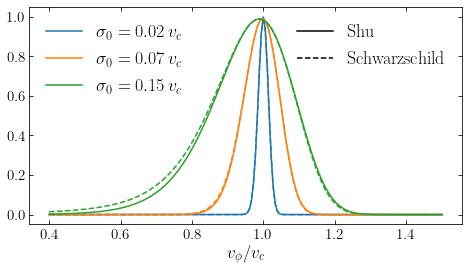
The velocity distribution for the Shu distribution function is displayed as the solid lines and that for the Schwarzschild distribution is shown as the dashed lines. It is clear for small velocity dispersion that the two distribution functions give essentially identical velocity distributions, but for the model with the largest \(\sigma_0\) the Schwarzschild distribution function gives a slightly wider velocity distribution and one that is slightly shifted toward smaller \(v_\phi\). The difference in the mean \(\overline{v_\phi}\) is nevertheless only about \(v_c/100\), so the difference is quite small. Of course in locations where the velocity dispersion is larger (e.g., \(R<1\) in the above example) the difference will be larger.
11.2.2.3. The Dehnen distribution function
Dehnen (1999) introduced a new disk distribution function by starting from a different form of the cold-disk distribution function. We can write the cold-disk distribution function alternatively as
where \(L_c(E)\) is the angular momentum of a circular orbit with energy \(E\) and \(\Omega(E)\) is the azimuthal frequency of that orbit. The argument of the delta function is in the epicycle approximation equal to \(E-E_c[L_z]\) and therefore given by
Following a similar calculation of \(\Sigma'(R)\) as in Section 11.2.1 above, we find that
where \(E_c[R]\) is the energy of a circular orbit at radius \(R\). Therefore, we can match a desired suface density \(\Sigma(R)\) by setting
where now \(R_E\) is the radius of a circular orbit with energy \(E\). An alternative form for the cold-disk distribution function in Equation \(\eqref{eq-colddisk-df}\) is therefore
Equation \(\eqref{eq-colddisk-df-alt}\) is the same distribution function as the cold-disk distribution function in Equation \(\eqref{eq-colddisk-df}\).
We can now build a disk distribution function with non-zero velocity dispersion by replacing the delta-function kernel in Equation \(\eqref{eq-colddisk-df-alt}\) with an exponential, just like how we created the Schwarzschild and Shu distribution functions starting from Equation \(\eqref{eq-colddisk-df}\). This gives the Dehnen disk distribution function
Dehnen (1999) argues that this distribution function more faithfully models the process through which stellar populations in a disk attain a non-zero velocity dispersion than the Shu distribution function does.
Let’s compare the Dehnen, Shu, and Schwarzschild distribution functions for the same model family \(\Sigma(R)\) and \(\sigma_R(R)\) as in Equations \(\eqref{eq-schwarzschilddf-examplefamily-1}\) and \(\eqref{eq-schwarzschilddf-examplefamily-2}\). The distribution of \(v_\phi\) at \(R=1\) is now given by
[15]:
from galpy.df import shudf, dehnendf, schwarzschilddf
df_cold_shu= shudf(profileParams=(1./3.,1.0,0.02),beta=0.)
df_warmer_shu= shudf(profileParams=(1./3.,1.0,0.07),beta=0.)
df_warm_shu= shudf(profileParams=(1./3.,1.0,0.15),beta=0.)
df_cold_dehnen= dehnendf(profileParams=(1./3.,1.0,0.02),beta=0.)
df_warmer_dehnen= dehnendf(profileParams=(1./3.,1.0,0.07),beta=0.)
df_warm_dehnen= dehnendf(profileParams=(1./3.,1.0,0.15),beta=0.)
df_cold_schwarz= schwarzschilddf(profileParams=(1./3.,1.0,0.02),beta=0.)
df_warmer_schwarz= schwarzschilddf(profileParams=(1./3.,1.0,0.07),beta=0.)
df_warm_schwarz= schwarzschilddf(profileParams=(1./3.,1.0,0.15),beta=0.)
vts= numpy.linspace(0.4,1.5,201)
figsize(7.75,4)
# Cold
ycold= numpy.array([df_cold_dehnen(numpy.array([1.,0.,vt])) for vt in vts])
norm= (numpy.amax(ycold)+numpy.random.uniform()/10.)
line_cold= plot(vts,ycold/norm,
                label=r'$\sigma_0 = 0.02\,v_c$')
ycold= numpy.array([df_cold_shu(numpy.array([1.,0.,vt])) for vt in vts])
plot(vts,ycold/norm,color=line_cold[0].get_color(),ls='--',zorder=0)
ycold= numpy.array([df_cold_schwarz(numpy.array([1.,0.,vt])) for vt in vts])
plot(vts,ycold/norm,color=line_cold[0].get_color(),ls=':',zorder=0)
# Warmer
ywarmer= numpy.array([df_warmer_dehnen(numpy.array([1.,0.,vt])) for vt in vts])
norm= (numpy.amax(ywarmer)+numpy.random.uniform()/10.)
line_warmer= plot(vts,ywarmer/norm,
                  label=r'$\sigma_0 = 0.07\,v_c$')
ywarmer= numpy.array([df_warmer_shu(numpy.array([1.,0.,vt])) for vt in vts])
plot(vts,ywarmer/norm,color=line_warmer[0].get_color(),ls='--',zorder=0)
ywarmer= numpy.array([df_warmer_schwarz(numpy.array([1.,0.,vt])) for vt in vts])
plot(vts,ywarmer/norm,color=line_cold[0].get_color(),ls=':',zorder=0)
# Warm
ywarm= numpy.array([df_warm_dehnen(numpy.array([1.,0.,vt])) for vt in vts])
norm= (numpy.amax(ywarm)+numpy.random.uniform()/10.)
line_warm= plot(vts,ywarm/norm,
                label=r'$\sigma_0 = 0.15\,v_c$')
ywarm= numpy.array([df_warm_shu(numpy.array([1.,0.,vt])) for vt in vts])
plot(vts,ywarm/norm,color=line_warm[0].get_color(),ls='--',zorder=0)
ywarm= numpy.array([df_warm_schwarz(numpy.array([1.,0.,vt])) for vt in vts])
plot(vts,ywarm/norm,color=line_cold[0].get_color(),ls=':',zorder=0)
xlabel(r'$v_\phi/v_c$')
# Schwarzschild and Shu legend entries
import matplotlib.lines as mlines
dehnen_line= mlines.Line2D([], [], color='k',marker=None,ls='-',
                        label=r'$\mathrm{Dehnen}$')
shu_line= mlines.Line2D([], [], color='k',marker=None,ls='--',
                        label=r'$\mathrm{Shu}$')
schwarzschild_line= mlines.Line2D([], [], color='k',marker=None,ls=':',
                        label=r'$\mathrm{Schwarzschild}$')
gca().add_artist(legend(handles=[dehnen_line,shu_line,schwarzschild_line],
                       loc='upper right',fontsize=18.,frameon=False))
legend(handles=[line_cold[0],line_warmer[0],line_warm[0]],
       fontsize=18.,loc='upper left',frameon=False);
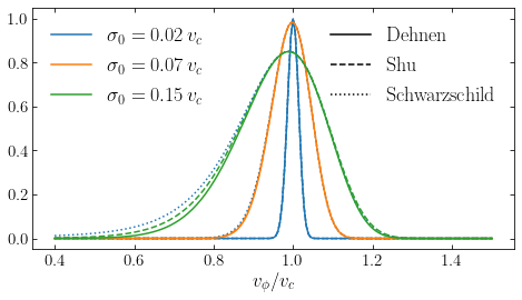
In this figure, the solid curves are for the Dehnen distribution function, the dashed for the Shu distribution function, and the dotted for the Schwarzschild distribution function. We see that all three distribution functions give essentially the same distribution of \(v_\phi\) for small \(\sigma_0\), but for the largest \(\sigma_0\), the Dehnen distribution function gives a narrower distribution than the other models. The difference between the Shu and Dehnen distribution functions is mostly due to the fact that the Dehnen distribution function has a smaller velocity dispersion \(\sigma'_R\) than the Shu distribution function for the same input \(\sigma_R\). The Dehnen model produces a better match between \(\Sigma'(R)\) and \(\Sigma(R)\) and between \(\sigma'_R(R)\) and \(\sigma_R(R)\). For example, for the warmest Dehnen model in the example above, the following figure shows \(\Sigma(R)\) compared to \(\Sigma'(R)\) and \(\sigma'_R(R)\) compared to \(\sigma_R(R)\):
[19]:
from galpy.df import dehnendf
df_warm_dehnen= dehnendf(profileParams=(1./3.,1.0,0.15),beta=0.)
Rs= numpy.linspace(0.1,2.,101)
figsize(10,4)
subplot(1,2,1)
sigmaprime= numpy.array([df_warm_dehnen.surfacemass(R) for R in Rs])
line_sprime= semilogy(Rs,sigmaprime,zorder=1,
                     label=r"$\Sigma'(R)$")
sigma= numpy.array([df_warm_dehnen.targetSurfacemass(R) for R in Rs])
line_sdens= semilogy(Rs,sigma,zorder=0,
                    label=r"$\Sigma(R)$")
xlabel(r'$R$')
xlim(0.,2.3)
legend(handles=[line_sprime[0],line_sdens[0]],
       fontsize=18.,loc='upper right',frameon=False)
subplot(1,2,2)
sigma2prime= numpy.array([df_warm_dehnen.sigma2(R) for R in Rs])
line_sprime= plot(Rs,numpy.sqrt(sigma2prime),zorder=1,
                     label=r"$\sigma_R'(R)/v_c$")
sigma2= numpy.array([df_warm_dehnen.targetSigma2(R) for R in Rs])
line_sigma2= plot(Rs,numpy.sqrt(sigma2),zorder=0,
                    label=r"$\sigma_R(R)/v_c$")
xlabel(r'$R$')
xlim(0.,2.3)
ylim(0.,0.4)
legend(handles=[line_sprime[0],line_sigma2[0]],
       fontsize=18.,loc='upper right',frameon=False);
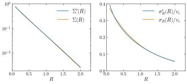
We see again that the match is very good (compare to that for the Schwarzschild distribution function above). Thus, the Dehnen distribution function more faithfully represents the desired surface density and velocity dispersion profile and this is typically the case over a range of models for \(\Sigma(R)\) and \(\sigma_R(R)\) and for different gravitational-potential models. Dehnen (1999) also provides an algorithm that can be applied to all warm disk distribution functions discussed here to iteratively change the input surface density and velocity dispersion profiles to attain a better match between \(\Sigma'(R)\) and \(\Sigma(R)\) and between \(\sigma'_R(R)\) and \(\sigma_R(R)\). An example of this is in the following figure, where we set \(\sigma_0 = 0.2\,v_c\) and run 20 iterations of Dehnen’s correction algorithm:
[13]:
from galpy.df import dehnendf
df_warm_dehnen= dehnendf(profileParams=(1./3.,1.0,0.2),beta=0.,correct=True)
Rs= numpy.linspace(0.1,2.,101)
sigmaprime= numpy.array([df_warm_dehnen.surfacemass(R) for R in Rs])
figsize(7,4)
line_sprime= semilogy(Rs,sigmaprime,zorder=1,
                     label=r"$\Sigma'(R)$")
sigma= numpy.array([df_warm_dehnen.targetSurfacemass(R) for R in Rs])
line_sdens= semilogy(Rs,sigma,zorder=0,
                    label=r"$\Sigma(R)$")
xlabel(r'$R$')
xlim(0.,2.3)
legend(handles=[line_sprime[0],line_sdens[0]],
       fontsize=18.,loc='upper right',frameon=False);
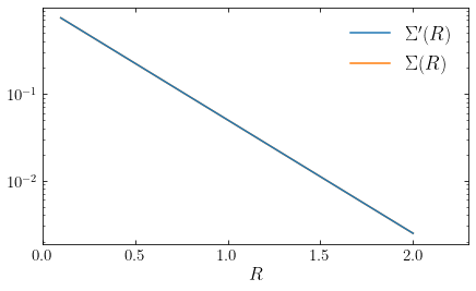
There is now essentially no difference between \(\Sigma'(R)\) and \(\Sigma(R)\) (the orange line is beneath the blue line everywhere).
11.3. The velocity distribution in the solar neighborhood
We can now use the axisymmetric Jeans equation and the distribution function models for disks that we have looked at in this chapter so far to attempt to understand the kinematics of stars in the solar neighborhood. We will focus here on the kinematics of stars near the Sun in the mid-plane of the disk, with velocities \((v_R,v_\phi)\) and discuss the vertical kinematics at the end of this chapter.
11.3.1. The asymmetric drift and the Sun’s motion
We start by using the axisymmetric, radial Jeans equation to understand the overall properties of the observed velocity distribution of different populations of stars. We measure the velocities of nearby stars by determining how fast stars move with respect to the Sun, either as the line-of-sight velocity measured as a Doppler shift or as the proper motion of a star on the sky. (Note that we directly observe the velocity with respect to the Earth [or with respect to a satellite, when making observations from space], but we know the Earth’s [or satellite’s] velocity well enough that we can correct measured velocities for the Earth’s motion; typically velocities are correct to the Solar System barycenter rather than to the Sun, but for galactic purposes the difference between these reference frames does not matter]. The axisymmetric Jeans equation applies to velocities in the Galactocentric coordinate frame, so to use them we need to correct for the Sun’s motion with respect to this frame. The Sun’s motion, however, is not known at high precision and some of the best contraints on it actually come from applying the axisymmetric Jeans equation.
As discussed in Appendix A.3, we can convert observed velocities to the Galactic coordinate system, where velocities are commonly denoted as \((U,V,W)\) (these are the velocities in the cartesian coordinate system of Galactic coordinates centered on the Sun). Because any observed star is not located exactly at the Sun’s location, we cannot, after accounting for the Sun’s motion, directly interpret \(U\) as minus the Galactocentric radial velocity or \(V\) as the Galactocentric azimuthal velocity as required by the axisymmetric Jeans equation. However, for stars that are close to the Sun, the difference is small and, moreover, we can use the Oort constants to correct a star’s velocity for the difference between a star’s position and the Sun’s position. Remember that the Oort constants, which we introduced in Chapter 9.4, describe the velocity field as a function of distance from the Sun to first order in the distance; using the measured Oort constants we can thus correct observed velocities for the effect of differential Galactic rotation to what they would be if observed at the exact position of the Sun, where \(U = -v_R+U_0\) and \(V = v_\phi + v_c(R_0) + V_0\) (where \(v_c(R_0)\) is the circular velocity at the Sun’s location and \([U_0,V_0]\) are the components of the Sun’s velocity with respect to a circular orbit at its location). This is most easily done at the level of the observed proper motions and line-of-sight velocities which get corrected as (see Equations 9.41, 9.42, and 9.43)
We then compute \((U,V,W)\) from the corrected velocities. Overall, this is a small correction for local stars and is therefore not that important, but it becomes more important when the distance increases. Typical random velocities of stars in the disk near the Sun are \(\gtrsim 10\,\mathrm{km\,s}^{-1}\); at a distance of 100 pc, this corresponds to a proper motion of \(100\,\mathrm{km\,s}^{-1}\,\mathrm{kpc}^{-1} \approx 20\,\mathrm{mas\,yr}^{-1}\) (because \(1\,\mathrm{mas\,yr}^{-1} \approx 5\,\mathrm{km\,s}^{-1}\,\mathrm{kpc}^{-1}\)). From the measured values of the Oort constants (see Chapter 9.4), the maximum correction in \(\mu_l\) is \(|A-B| \approx 27\,\mathrm{km\,s}^{-1}\,\mathrm{kpc}^{-1} \approx 5.5\,\mathrm{mas\,yr}^{-1}\) and the maximum correction in \(\mu_b\) is even smaller. The correction is therefore much smaller than the typical random motion.
We can then re-write the Stromberg asymmetric drift Equation \(\eqref{eq-stromberg}\) in terms of \(U\) and \(V\), assuming that the Milky Way is axisymmetric and therefore \(\overline{v_R^2} = \sigma_R^2 = \sigma_U^2\) and \(\overline{v_R v_z} = \sigma_{UW}^2\)
From the fact that the planar and vertical components of the orbital motion are approximately decoupled for disk orbits, we expect \(\sigma_{UW}^2\) to vanish. Observations of the full velocity distribution indeed show that this is the case (see below). Everything in the equation above is then directly observable, except for \(V_0\) and \(v_c\).
The solar neighborhood is made up of stars with ages between zero and about 12 Gyr. Because of interactions with, for example, molecular clouds and spiral structure, older stars have larger velocity dispersions \(\sigma_U\). From Equation \(\eqref{eq-stromberg-obs}\), it is clear that they will have a different value of \(-\overline{V}-V_0\). The two main unknowns in Equation \(\eqref{eq-stromberg-obs}\), \(V_0\) and \(v_c\), should be the same no matter what population we use to determine them (at least if the Milky Way is axisymmetric, which was the main assumption behind Equation \(\ref{eq-stromberg-obs}\)). Therefore, we can use the kinematics of different populations of stars to determine \(V_0\) and \(v_c\).
Using Equation \(\eqref{eq-stromberg-obs}\) to determine \(V_0\) and \(v_c\) from a single population of stars is difficult, because it requires measuring all of the terms within square brackets. The second of these involves the radial gradient of the density and of the velocity dispersion, which are difficult to determine from a local sample of stars. People have therefore attempted to get around measuring the factor in square brackets, by considering the observed relation between \(\overline{V}\) and \(\sigma_U^2\). If it appears that there is a simple relation between these two quantities, then we could parameterize this relation and essentially fit for the value of the square brackets. However, proceeding along this line means that we lose the ability to determine \(v_c\), because it is degenerate with the quantity in square brackets if we do not directly measure the quantity in square brackets. Because much interesting dynamics can be done in the solar neighborhood, but this requires one to correct for the Sun’s motion, only determining \(V_0\) is still very interesting.
Dehnen & Binney (1998) performed this type of measurement using the Hipparcos data (HIPPARCOS Collaboration 1997). Hipparcos was a satellite similar to the more recent Gaia satellite and Hipparcos observed about 120,000 stars over a few years around 1990 to measure their parallaxes and proper motions. Line-of-sight velocities were not available for the stars in the same selected by Dehnen & Binney (1998), so they had to deproject. This deprojection is possible for a sample surrounding the Sun, because each proper motion measurement gives a different projection of the same three-dimensional velocity distribution. They measured \(\overline{V}\), as well as \(\overline{U}\) and \(\overline{W}\) which in an axisymmetric Galaxy should simply reflect the Sun’s motion: \(\overline{U} = -U_0\) and \(\overline{W} = -W_0\), because \(\overline{v_R} = \overline{v_z} = 0\). They performed this measurement for different samples of stars along the main sequence selected using the \(B-V\) color, which is correlated with the mean age of the population.
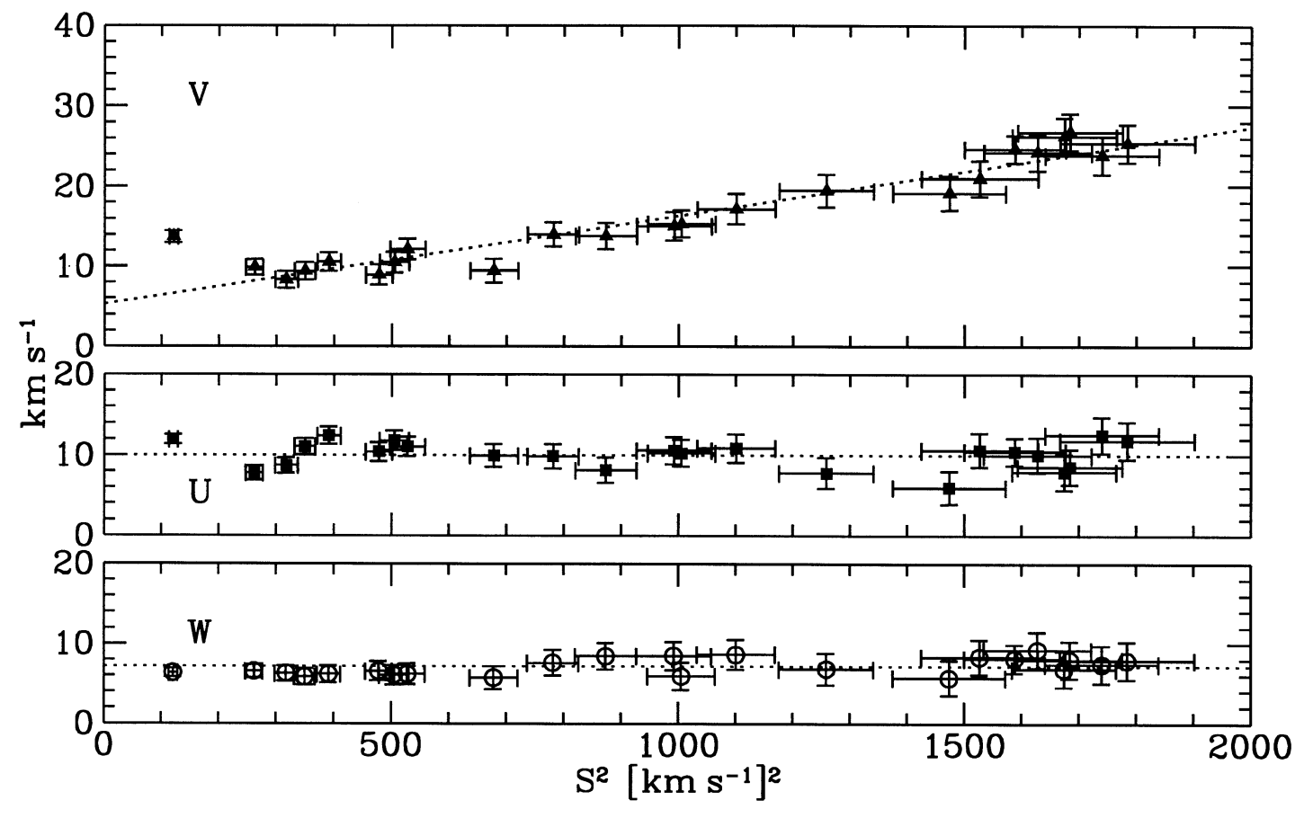
The following figure displays their basic measurements of \(-\overline{V}\), \(-\overline{U}\), and \(-\overline{W}\) versus \(B-V\) (they display minus the mean, because this is directly equal to the Sun’s motion for \(U\) and \(W\) and equal to the Sun’s motion for \(\sigma_U = 0\) for \(V\)):
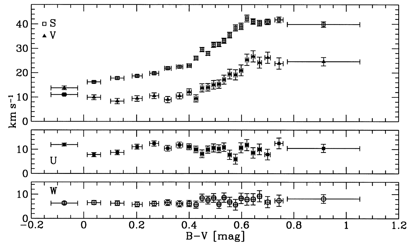
(Credit: Dehnen & Binney 1998)
As expected, there is no trend with \(B-V\) in \(-\overline{U}\) and \(-\overline{W}\) and we can combine the measurements from each population to estimate \(U_0\) and \(W_0\). This gives
The measurement of \(-\overline{V}\) does display a trend with \(B-V\). The squares in the top panel give a measurement of \(S^2\), which is a measure of the velocity dispersion squared (\(S^2 \propto \sigma_U^2\), but not equal; this was a convenient quantity to determine in the process of deprojecting the proper motions). It is clear that \(\overline{V}\) and \(S^2\) trace each other, as expected from the asymmetric drift equation in the form of Equation \(\eqref{eq-stromberg-obs}\). The following figure shows \(-\overline{V}\) (and the other components as well) as a function of \(S^2 \propto \sigma_U^2\)
(Credit: Dehnen & Binney 1998)
From this it appears that there is a linear relation between \(\overline{V}\) and \(S^2\). This type of relation would make sense from Equation \(\eqref{eq-stromberg-obs}\) if the quantity in the square brackets does not depend on \(B-V\), that is, if it is the same for all stellar populations. This would appear to be a reasonable assumption: the ratio \(\sigma_V^2/\sigma_U^2 = B/(B-A)\) in the epicycle approximation and does not vary much as the velocity dispersion increases; similarly, it is not unreasonable to assume that stars have similar density distribution \(\nu(R)\) and dispersion profiles \(\sigma_U(R)\), such that the derivate in the second term should not vary much. Therefore, if we assume that the quantity in square brackets is constant, then we can fit for a linear relation between \(-\overline{V}\) and \(S^2\) and the intercept at \(S^2 = 0\) of this relation will be equal to \(V_0\). This is the fit that is shown as a dotted line in the figure above and it gives
Even though there clearly seems to be a linear relation between \(\overline{V}\) and \(\sigma_U^2\), this linear relation is likely spurious and leads to an incorrect value of \(V_0\). This is because according to our current best understanding of the structure of the Milky Way’s disk, the quantity in square brackets in Equation \(\eqref{eq-stromberg-obs}\) is not constant, but is different for different stellar populations. In particular, we now know that the Milky Way disk consists of a large number of populations with very different spatial densities. These densities \(\nu(R,z)\) are different enough to make a large difference in the quantity in square brackets.
A good illustration of this point is given by the decomposition of the Milky Way’s stellar surface density into stellar populations separated by age, metallicity, and alpha-enhancement by Mackereth et al. (2017) (see Chapter 12 for a discussion of the metallicity and alpha-enhancement of stars). This is shown in the following figure
![Figure 6 from Mackereth et al. (2017): Disk surface density distributions of stellar populations separated by [a/Fe], [Fe/H], and age Sun](../_images/mackereth17_figure6.png)
(Credit: Mackereth et al. 2017)
The level of transparency in this figure indicates the relative importance of each metallicity component in a given age bin (darker bands have more stars near the Sun than more transparent bands). The first thing to notice is that many populations do not look like simple exponential distributions, but instead have a radius at which the surface density peaks (first discovered by Bovy et al. 2016). Secondly, while for older, low-[\(\alpha\)/Fe] and for high-[\(\alpha\)/Fe] stars the surface density is declining around \(R_0 = 8\,\mathrm{kpc}\), for many of the younger populations the peak in the surface density is at \(R > R_0\) and the surface density near the Sun is increasing for these populations. As we discussed in Section 11.2.2.1 above, this behavior leads to a negative asymmetric drift (that is, \(\overline{v_\phi} > v_c\) as opposed to the “normal” \(\overline{v_\phi} < v_c\) behavior). It is clear that this type of behavior wreaks havoc on efforts to approximate Stromberg’s asymmetric drift equation as a linear relation bewteen \(\overline{V}\) and \(\sigma_U^2\)!
This effect was first pointed out by Schönrich et al. (2010), by looking at the relation between \(\overline{V}\) and \(\sigma_U^2\) in a model for the Milky Way disk that includes chemical evolution and the growth and kinematics of different stellar populations (developed by Schönrich & Binney 2009). The following figure displays the relation between \(-\overline{V}\) and \(\sigma_U^2\) in this model, which has \(V_0 = 0\) as the green squares:
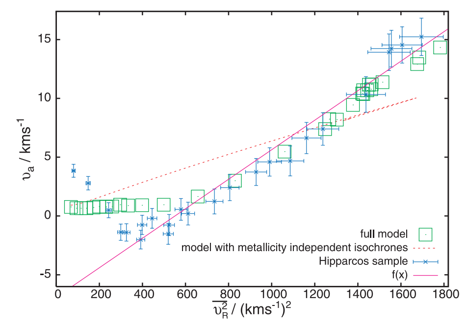
(Credit: Schönrich et al. 2010)
A version of the Hipparcos results is included as the blue points with errorbars (these points are shifted by \(V_0 = 11\,\mathrm{km\,s}^{-1}\) to better agree with the model). At large values of \(\sigma_U^2\), the model follows the same type of linear relation as the model, but at small values of \(\sigma_U^2\) the model has a constant value of \(\overline{V}\). This is because the populations that have small \(\sigma_U^2\) are the populations which have a density profile that is flat or increasing near the Sun, and such populations have a small asymmetric drift or even a slightly negative one.
To see how this happens in a simple model, we can use the Dehnen distribution functions from Section 11.2.2.3 above to simulate stellar populations in the solar neighborhood. We simulate 25 populations with \(\sigma_R(R_0)/v_c\) between \(0.01\) and \(0.2\) (that is, \(\sigma_R(R_0)\) ranging from \(\approx 2\,\mathrm{km\,s}^{-1}\) to \(\approx 45\,\mathrm{km\,s}^{-1}\)) in a potential with a flat rotation curve. We assume that every
population has \(\sigma_R(R) = \sigma_R(R_0)\,e^{-R/R_0}\) and that \(\Sigma(R) \propto e^{-R/h_R}\). We then consider two cases: (i) \(h_R = R_0/3\) for all populations (thus, the scale length is \(\approx 2.7\,\mathrm{kpc}\), a reasonable value for stars in the disk of the Milky Way), and (ii) the scale length transitions from \(h_R = R_0/3\) at large \(\sigma_R\) to \(h_R = -R_0/3\) at small \(\sigma_R\) (we transition the scale length with a tanh function
of \(1/h_R\) to go through a flat profile around \(\sigma_R^2 = 500\,\mathrm{km\,s}^{-1}\)):
[21]:
from galpy.df import dehnendf
vo= 220. # to scale velocities to km/s
srs= numpy.linspace(0.01,0.2,25)
# First do case where h_r = 1./3. everywhere
hrs= 1./3.*numpy.ones_like(srs)
vas_hrconst= numpy.empty_like(srs)
for ii,(sr,hr) in enumerate(zip(srs,hrs)):
    df= dehnendf(profileParams=(hr,1.0,sr),beta=0.)
    vas_hrconst[ii]= 1.-df.meanvT(1.)
figsize(7.5,4)
line_hrconst= plot(srs**2.*vo**2.,vas_hrconst*vo,'o',
                   label=r'$h_R = R_0/3$')
# Now do case where h_r varies
hrs= 1./(numpy.tanh((srs-0.1)/0.008)*3)
hrs[srs > 0.1]= 1./(numpy.tanh((srs[srs > 0.1]-0.1)/0.05)*3)
vas_hrtrend= numpy.empty_like(srs)
for ii,(sr,hr) in enumerate(zip(srs,hrs)):
    df= dehnendf(profileParams=(hr,1.0,sr),beta=0.)
    vas_hrtrend[ii]= 1.-df.meanvT(1.)
line_hrtrend= plot(srs**2.*vo**2.,vas_hrtrend*vo,'s',
    markerfacecolor='none',
    label=r'$1/h_R = \mathrm{between}\ -3/R_0\ \&\ 3/R_0$')
xlabel(r'$\sigma_R^2\,(\mathrm{km}^2\,\mathrm{s}^{-2})$')
ylabel(r'$v_c-\overline{v_\phi}\,(\mathrm{km\,s}^{-1})$')
xlim(-1.,1850.)
ylim(-6.,19.99)
legend(handles=[line_hrconst[0],line_hrtrend[0]],
       fontsize=17.,loc='upper left',frameon=False);
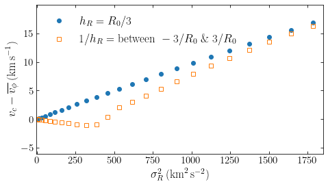
When the scale length is constant, we get the expected linear behavior between the asymmetric drift and the velocity dispersion squared. But when the scale length is variable and becomes negative (corresponding to an increasing density for those populations near the Sun), we see that we get the same behavior as in the complicated chemical-evolution model discussed above: the asymmetric drift becomes slightly negative around zero once the radial density becomes flat or increasing at the solar circle.
By adjusting the solar motion component \(V_0\) in their chemical evolution model, Schönrich et al. (2010) found a best-fit between their model and the observed kinematics of stars in the solar neighborhood of
with a significant contribution from systematics related to the complexity of the velocity distribution (see below).
The asymmetric drift, while a simple consequence of the equilibrium dynamics of stellar disks, therefore manifests itself in complicated ways in galactic disks. This is because of its dependence on the radial profile of the density of stellar populations, which has complicated trends for different populations due to the complex formation and evolution history of the galactic disks.
11.3.2. The distribution of velocities in the solar neighborhood
The discussion of the kinematics of stars in the solar neighborhood so far has focused solely on the behavior of the mean velocity in different directions, using the axisymmetric, radial Jeans equation to provide the equilibrium interpretation. But we have sufficient data on velocities of stars in the solar neighborhood to investigate the full three-dimensional distribution of velocities and compare it to the predictions from the equilibrium distribution function models in Section 11.2.
The first unbiased determinations of the three-dimensional velocity distribution of stars near the Sun was made possible by observations taken with the Hipparcos satellite and we are now able to look at this distribution in more detail with data from the Gaia satellite. For the purposes of our discussion here, the velocity distribution derived from Gaia data is essentially the same as that coming from Hipparcos. As mentioned above, Hipparcos only measures the proper motion of stars, not their line-of-sight velocities, and therefore we need to de-project the two-dimensional observations assuming that the local velocity distribution is the same in all directions (a good assumption). We will not go into the details of how this can be done here, but will merely discuss the results and we will see that the full 3D data from Gaia agrees with the de-projected Hipparcos results. In this section, we focus on the in-plane velocity distribution, that is, the distribution of \((U,V)\) (which many of the authors mentioned below will often denote as \((v_x,v_y)\)).
Before looking at the measured velocity distribution, we use a Dehnen distribution function from Section 11.2.2.3 above to predict the distribution that we should see for an equilibrium, axisymmetric disk. From the discussion in Section 11.2.2.1, we know that for close-to-circular orbits, all of the distribution functions that we discussed above will be approximately Gaussian. But let’s plot the velocity distribution for a population of stars with \(\sigma_R(R_0) = 30\,\mathrm{km\,s}^{-1}\), a value appropriate for the few Gyr old stars in the solar neighborhood that make up the bulk of the Hipparcos sample (for simplicity, we again assume \(\Sigma(R) \propto e^{-R/h_R}\) with \(h_R = R_0/3\) and \(\sigma_R(R) \propto e^{-R/R_0}\), and we use a flat rotation curve).
[23]:
from galpy.df import dehnendf
vo= 220. # to scale velocities to km/s
sr= 30./vo
df= dehnendf(profileParams=(1./3.,1.0,sr),beta=0.)
vRmin, vRmax= -120./vo,120./vo # vR = -U
vTmin, vTmax= 1.-120./vo, 1.+60./vo # vT, not V
nvR= 101
nvT= 102
vRs= numpy.linspace(vRmin,vRmax,nvR)
vTs= numpy.linspace(vTmin,vTmax,nvT)
vdf= numpy.empty((nvR,nvT))
for ii,vR in enumerate(vRs):
    for jj,vT in enumerate(vTs):
        vdf[ii,jj]= df(numpy.array([1.,-vR-10./vo,vT+12.24/vo]))
figsize(6,6)
galpy_plot.dens2d(vdf.T,origin='lower',cmap='gist_yarg',
                  xlabel=r'$U\,(\mathrm{km\,s}^{-1})$',
                  ylabel=r'$V\,(\mathrm{km\,s}^{-1})$',
                  contours=True,cntrmass=True,
                  levels=numpy.array([2,6,12,21,33,50,68,
                                      80,90,95,99,99.9])/100.,
                  cntrcolors=['0.9','0.8','0.7','0.6','0.5',
                              '0.4','0.3','0.2','0.1','0.',
                              'k','k'],
                  xrange=[(-vRmax-0.5*(vRs[1]-vRs[0]))*vo,
                          (-vRmin+0.5*(vRs[1]-vRs[0]))*vo],
                  yrange=[(vTmin-0.5*(vTs[1]-vTs[0])-1.)*vo,
                          (vTmax+0.5*(vTs[1]-vTs[0])-1.)*vo]);
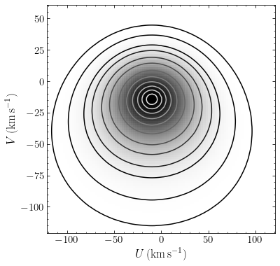
The contour levels here contain (2, 6, 12, 21, 33, 50, 68, 80, 90, 95, 99, and 99.9) % of the distribution and are the same as those in the observational determinations below. We have also shifted the velocity distribution to heliocentric coordinates using the solar motion discussed in the previous section.
The properties and shape of this distribution are as expected. Overall, the distribution is close to Gaussian and is symmetric around the \(v_R = 0\) line (which falls at \(U = -10\,\mathrm{km\,s}^{-1}\) in heliocentric coordinates). The effect from the asymmetric drift shifts the peak away from \(v_\phi = v_c\) and causes the \(V\) distribution to be skewed: the velocity distribution extends to much more negative values than it extends to positive values. The velocity distribution is smooth. Even when we mix multiple populations with different values of \(\sigma_R(R_0)\) and/or \(\Sigma(R)\) and \(\sigma_R(R)\), we would still expect a similar shape, with similar smoothness. Observationally, the properties of the local velocity distribution are sometimes summarized using the velocity ellipsoid, which is its covariance matrix
where the second equality holds in the solar neighborhood, but the first equality is the general form. Because a covariance matrix describes an ellipsoidal shape, the off-diagonal components are generally expressed as angles representing the angles of this ellipsoid with respect to the coordinate axes; The angle \(l_V\) associated with \(\sigma_{R\phi}^2\) is the vertex deviation and is given by
The angle associated with \(\sigma_{Rz}^2\) is the tilt of the velocity ellipsoid and is discussed in further detail in Section 11.4.1 below. The steady-state, axisymmetric prediction is that the vertex deviation is equal to zero: \(l_V = 0\) and \(\sigma_{R\phi}^2 = 0\).
The next figure displays the observed velocity distribution, as determined by Dehnen (1998) from Hipparcos data and by Gaia Collaboration et al. (2018) using the more recent Gaia data:
|
|
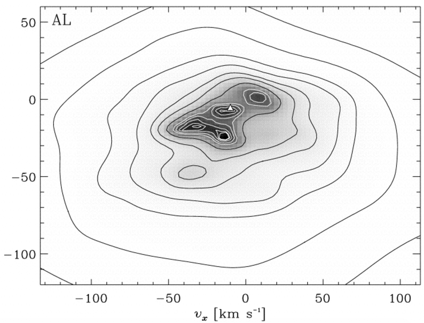
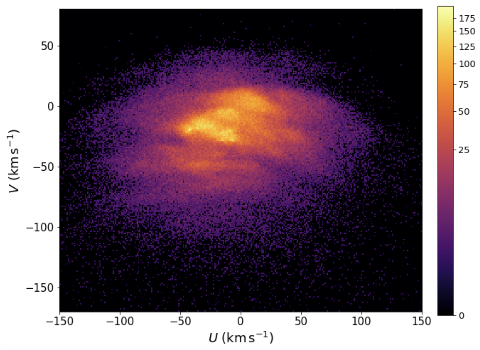
(Credit: left: Dehnen 1998; right: Gaia Collaboration et al. 2018)
We see that this distribution is quite different from that expected for an equilibrium, axisymmetric disk: rather than being a smooth distribution that is symmetric around \(v_R = 0\), the distribution is characterized by many overdensities and a vertex deviation of \(l_V \approx 10^\circ\). The deprojection technique used by Dehnen makes it difficult to interpret the significance of all of the features in the observed velocity distribution, but the Gaia data beautifully confirm that the main overdensities are real and that they, in fact, have further small-scale structure. Most of the structures seen in the velocity distribution—which are known as moving groups—had been known before Hipparcos from previous determinations of the velocity distribution (e.g., Boss 1908; Hertzsprung 1909; Roman 1949; Ogorodnikov & Latyshev 1968; Eggen 1970), but it had not been clear how prominent they were until the Hipparcos results. Bovy et al. (2009) find that about 40% of local stars are contained in the main moving groups. This is a very significant number of stars!
The observed velocity distribution, with its prominent moving groups, is therefore very different from that expected for a steady-state galaxy. Because the moving groups contain many stars and those stars have a wide range of ages and metallicities (e.g., Famaey et al. 2005; Bensby et al. 2007; Bovy & Hogg 2010), it is very unlikely that they are clusters of stars born together that are still in the process of becoming a phase-mixed, equilibrium population De Simone et al. (2004). They are most likely due to the effect of time-dependent, non-axisymmetric perturbations to the Galactic potential, such as those from the bar and spiral structure (e.g., Dehnen 2000; De Simone et al. 2004; Hunt et al. 2019).
11.4. The vertical equilibrium state of disks
We now turn to a discussion of the vertical equilibrium of galactic disks. Like for the equilibrium states in the disk’s mid-plane, we will learn many useful things about the vertical equilibrium by working in the approximation that the vertical motion is decoupled from the planar motion in galactic disks, which is a good assumption for orbits that do not venture too far from the mid-plane (Chapter 10.2). For the vertical motion this leads to an especially simple system: the system is one-dimensional, with a two-dimensional phase-space \((q,p) = (z,v_z)\), and the vertical specific energy \(E_z = v_z^2/2 + \Phi_z(z)\) is an integral of the motion. The equilibrium collisionless Boltzmann equation for this one-dimensional system is
or in cartesian coordinates
Because the vertical energy is an integral of the motion, any function that only depends on the phase-space coordinates through the energy, \(f(z,v_z) \equiv f(E_z[z,v_z])\), is a solution of the equilibrium collisionless Boltzmann equation. Conversely, because phase-space is only two-dimensional, any equilibrium solution only depends on the phase-space coordinates through the vertical energy. Therefore, we only need to consider functions of the vertical energy to study equilibrium solutions (of course, we can consider other integrals as well, but these are all functions of the vertical energy).
Multiplying Equation \(\eqref{eq-equil-boltzmann-1d}\) by \(v_z\) and integrating over all \(v_z\) gives the decoupled axisymmetric, vertical Jeans Equation
Comparing this equation to the general axisymmetric, vertical Jeans Equation \(\eqref{eq-jeans-vertical-axi}\), we see that the term involving \(\overline{v_R\,v_z}\) is missing; this is because we have assumed that the vertical motion is decoupled from the planar motion, so \(\overline{v_R\,v_z} = 0\) (see also Equation \ref{eq-diskequil-axijeans-decoupledvertical-1}).
As we already discussed in Chapter 10.3.1, the Poisson equation takes on an approximate special form in galactic disks. Therefore, the vertical dynamics of galactic disks is approximately a truly one-dimensional dynamical system. The Poisson equation in cylindrical coordinates is
In many galactic disks, \(\frac{\mathrm{d} v_c^2}{\mathrm{d} R} \approx 0\), because their rotation curves are close to flat. But more generally, at a given \(R\), the first term on the right-hand side in Equation \(\eqref{eq-poisson-vertical}\) is very close to a constant up to multiple kpc for galactic mass distribution, even when it is non-zero (this was demonstrated using very general arguments by Bovy & Tremaine 2012). Thus, the first term gives rise to a small “phantom density” \(4\pi\,G\,\rho_\mathrm{RC}(R) = \frac{1}{R}\,\frac{\mathrm{d} v_c^2}{\mathrm{d} R}\) and we obtain a one-dimensional version (that is, at a constant radius) of the Poisson equation in galactic disks
We can also write the phantom density in terms of the Oort constants
As we did for the distribution function in the disk mid-plane in the first part of this chapter, we start by discussing the axisymmetric, vertical Jeans equation in more detail (including its non-decoupled form of Equation \ref{eq-jeans-vertical-axi}) before going on to full phase-space distribution function models.
11.4.1. The vertical Jeans equation
Many analyses of the vertical kinematics in galactic disks—most productively done in the solar neighborhood—make use of the vertical Jeans equation. We can re-write Equation \(\eqref{eq-jeans-vertical-axi}\) to provide the gravitational force \(-\frac{\partial \Phi}{\partial z}\) in terms of the density and velocity dispersions (we substitute \(\sigma_z^2 = \overline{v_z^2}\) and \(\sigma_{Rz}^2 = \overline{v_R\,v_z}\), because in an equilibrium, axisymmetric system, \(\overline{v_R} = \overline{v_z} = 0\))
Given observations at a given \(R\) of the tracer-density profile \(\nu(z)\) and the velocity-dispersion profile \(\sigma_z(z)\), we can directly determine the vertical component of the gravitational field \(g_z(z;R) = -\frac{\partial \Phi}{\partial z}\) at \(R\), but this further requires knowledge of \(\frac{\partial [R\,\nu\,\sigma^2_{Rz}]}{\partial R}\). This latter information has historically been difficult to obtain directly (although with Gaia data it should be possible to measure it directly as well) and the typical approach has been to make assumptions about it. This term is generally known as the tilt of the velocity ellipsoid, because when we consider \(\sigma^2_{Rz}\) as an entry in the velocity dispersion tensor of Equation \eqref{eq-diskequil-velellipsoid}, it can be equivalently be parameterized as an angle \(\alpha\) of the angle between the velocity’s ellipsoid and the \(z\) axis:
One assumption about the tilt of the velocity ellipsoid that we have already used many times is that the vertical motion is decoupled from the planar motion, because then \(\sigma^2_{Rz} = 0\) and, thus, \(\alpha = 0\) and we are left with the decoupled vertical Jeans equation (Equation \(\ref{eq-jeans-vertical-decoupled}\)). Another assumption, more appropriate for non-disk orbits is that on average stars move in a spherical potential. In that case the velocity ellipsoid “points towards the Galactic center” at all heights and, thus, \(\tan \alpha = z/R\). “Points towards the Galactic center” here means that the velocity ellipsoid tensor is aligned—that is, diagonal—in spherical coordinates, which is the case for all spherical distribution functions that we discussed in Chapter 6.6, including those with non-zero orbital anisotropy (which only affects the relative magnitude of the diagonal elements). Intermediate to these possibilities is that the motion decouples in a set of spheroidal components, e.g., in confocal prolate coordinates with foci at \((R,z) = (0,\pm \Delta)\) for some constant \(\Delta\) (e.g., de Zeeuw 1985; Binney 2012a; see Chapter 13 for more discussion of this coordinate system); then the velocity ellipsoid will be aligned with the coordinate axes in the spheroidal coordinate system, which can be chosen to be intermediate between \(\alpha = 0\) and \(\tan \alpha = z/R\). Of course, the velocity ellipsoid does not have to be globally diagonal (that is, at all positions) in any coordinate system!
While the tilt term is an unknown quantity that one needs to make assumptions about, even in the extreme case where the velocity dispersion tensor points to the Galactic center, the tilt term in Equation \(\eqref{eq-jeans-vertical-force}\) is smaller by a factor of about a hundred—for solar-neighborhood populations—than the first term on the right-hand side in Equation \(\eqref{eq-jeans-vertical-force}\) at \(|z| \lesssim 1\,\mathrm{kpc}\) (Zhang et al. 2013), and it can therefore be largely ignored when analyzing data close to the Galactic mid-plane. This is again a statement about the fact that the vertical motion approximately decouples from the planar motion, which is an especially good assumption to make about distributions of orbits.
We can combine the vertical Jeans equation with the Poisson equation to directly relate the mass distribution to the observed density and velocity dispersion. First, we integrate Equation \(\eqref{eq-poisson-vertical}\) to obtain a version of the Poisson equation that relates \(\Sigma(z;R)\), the surface density between \(-z\) and \(z\)—which we will refer to as the surface density up to height \(z\)—to the gravitational potential
where we have assumed that the mass distribution is symmetric for \(z \rightarrow -z\). Substituting \(\partial \Phi / \partial z\) from Equation \(\eqref{eq-jeans-vertical-force}\) and using the approximate, constant, form of the integrand from Equation \(\eqref{eq-phantomdens-oort}\), we find
This equation demonstrates that we rather directly constrain the surface density up to height \(z\) when we measure the stellar density profile \(\nu(z)\) and the kinematics around height \(z\). We will discuss applications of the vertical Jeans equation to the kinematics in the solar neighborhood in Section 11.4.4 below.
11.4.2. The vertical equilibrium of a self-gravitating disk
As a first set of solutions of Equation \(\eqref{eq-equil-boltzmann-1d}\), we consider distribution functions of the form
This is simply the one-dimensional version of the isothermal sphere that we investigated in Chapter 6.6.2 and it is also similar to all of the razor-thin disk distributions that we considered above (which all become exponentials of minus the epicycle energy for nearly circular orbits). Like the isothermal sphere, the velocity distribution of this distribution function is Gaussian at all \(z\)
The density is an exponential of minus the potential
These results are valid for any isothermal distribution function in a given potential \(\Phi_z(z)\).
If we also require self-consistency—that the potential is sourced by the density implied by the distribution function—we have an additional constraint from the Poisson equation, which in one dimension is
where \(\rho(z) = \nu(z)\) given above. A self-consistent, isothermal galactic disk therefore satisfies
This equation is solved by the following potential–density pair
where \(H^2 = \sigma^2/[8\pi\,G\,\rho_0]\) or, alternatively, \(H = \sigma^2/[2\pi\,G\,\Sigma]\), where \(\Sigma = 4\,\rho_0\,H\) is the total surface density. This is the self-gravitating, isothermal sheet (“sheet”, because the decoupled vertical dynamics in a disk is that of sheets; Cuperman et al. 1969; Schulz et al. 2013).
11.4.3. The vertical distribution function for a given density profile
Similar to what we did for spherical ergodic distribution functions in Chapter 6.6.1, we can ask what the equilibrium vertical distribution function \(f(E_z)\) for a population with a given density \(\nu(z)\) orbiting in a vertically-decoupled gravitational field specified by the potential \(\Phi_z(z)\) is. Using a procedure analogous to that followed in Chapter 6.6.1, we determine this equilibrium distribution function here.
The density \(\nu(z)\) is given by the integral of the distribution function over velocity
Like for a spherical potential, for a one-dimensional potential, we can invert the relation \(\Phi_z(z)\) (at least at \(z > 0\); because we assume that the disk is symmetric around the mid-plane, \(\Phi_z(z) = \Psi\) has two solutions, one at \(z_\Psi\) and one at \(-z_\Psi\)) and we can write the density as a function of \(\Phi_z\) instead
This is an Abel integral equation, which can be inverted as
The distribution function obtained using Equation \(\eqref{eq-verticaldf-fordens}\) is the unique equilibrium distribution function for a given density \(\nu\) in a given potential \(\Phi_z\). If we have a well-measured density profile \(\nu(z)\) of a population of stars in the solar neighborhood, we can use Equation \(\eqref{eq-verticaldf-fordens}\) to determine the equilibrium distribution function for different potentials and compare the velocity distribution that these distribution functions predict with the observed kinematics to find the best matching potential.
11.4.4. The vertical equilibrium in the solar neighborhood
11.4.4.1. The local density of matter
We can roughly separate the types of analyses of the vertical density and kinematics in the solar neighborhood into two main classes: those that look at stars at \(|z| \ll z_d\), that is, less than the (mass-weighted) scale height of the stellar disk (\(z_d \approx 300\,\mathrm{pc}\) and those that look at stars with larger vertical excursions. In the first type, we can approximate the vertical density as being approximately constant \(\rho(z) \approx \rho_0 = \mathrm{constant}\); this type of analysis is known as the “Oort limit”, after Oort who was the first to perform this type of analysis in Oort (1932). Under this assumption the Poisson Equation \(\eqref{eq-poisson-vertical}\) is solved by the potential
where \(\omega^2 = 4\pi\,G\,[\rho_0+\rho_\mathrm{RC}(R)]\), including a possible contribution from the phantom density for a non-flat rotation curve (see the beginning of Section 11.4). A possible linear term in \(z\) in \(\Phi_z(z)\) must be zero if the potential is symmetric around \(z=0\) and we have fixed the constant such that \(\Phi_z(0) = 0\). Thus, close to the plane, the gravitational potential is approximately that of a harmonic oscillator centered on \(z=0\).
More generally, we can measure \(\Sigma(z;R)\) using the Jeans-equation method from Equation \(\eqref{eq-surfdens-fromverticaljeans}\). At small \(z\) where the density is approximately constant, \(\Sigma(z;R) = 2\,\rho_0\,z\) and we can thus obtain the local density from the slope of \(\Sigma(z;R)\). If the rotation curve is flat, \(\Sigma(z;R) = g_z(z)/[2\pi\,G]\) and then we can obtain the local density from the slope of the vertical gravitational field \(g_z(z)\) with \(z\).
Analyses of the vertical kinematics of this form have a long and venerable history. We will only discuss some highlights of this history here. The first analysis of this type was done by Oort (1932). This paper was also the first to discuss “dark matter” as a missing mass to account for the discrepancy between the amount of mass inferred from star light and that inferred from dynamics (Zwicky’s paper on the Coma cluster only appeared a year later). Oort (1932) used the vertical Jeans equation in the form of Equation \(\eqref{eq-jeans-vertical-force}\) with zero tilt (that is, without the second term on the right-hand side; his Equation 9) to determine the vertical field (or acceleration; \(K\) in his notation) \(g_z(z) = -\frac{\partial \Phi}{\partial z}\) from observations of \(\nu(z)\) (which he called \(\Delta\)) and \(\sigma_z^2\) (which he called \(\overline{Z^2}\)) of local stars. His measurement is displayed in his Figure 4:
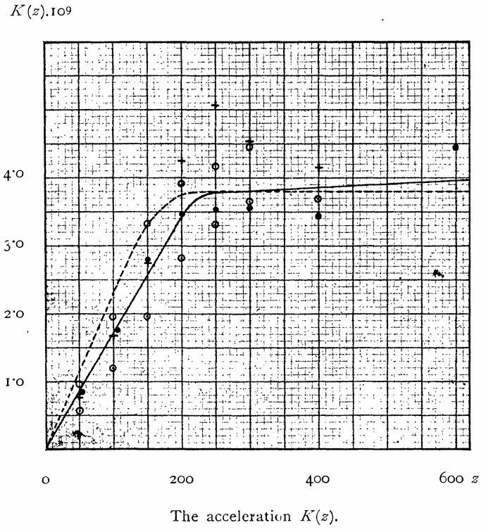
(Credit: Oort 1932)
The horizontal axis shows the vertical height \(z\) in pc, while the vertical axis shows \(g_z\) in units of \(10^{-9}\,\mathrm{cm\,s}^{-2}\). To be able to quickly interpret the measurements in this and the next section, the following unit conversions are useful
We can thus directly read off Oort’s measurement of the local density \(\rho_0\) (assuming a flat rotation curve, so no phantom density) from his measurement of \(g_z(z)\) (using the point at \(z=200\,\mathrm{pc}\) to estimate the slope):
This value is in fact still the accepted value, as we will see below. Oort (1932) compared this value to his best estimate of visible matter, which was \(\rho_{\mathrm{vis}} \approx 0.04\,M_\odot\,\mathrm{pc}^{-3}\) and invoked “dark matter” to explain the discrepancy between the two. While this is (arguably, as with all things) the first use of “dark matter” to explain the discrepancy between mass-to-light-ratio-estimated mass and dynamically-esimated mass, Oort was well aware of the fact that this missing mass was most likely made up of (i) numerous faint stars below the detection limit and (ii) instellar gas. Current inventories of the solar neighborhood indeed show that all of the \(\rho_0 = 0.1\,M_\odot\,\mathrm{pc}^{-3}\) local density is accounted for by stars and gas (with just enough uncertainty to allow for the small amount of halo dark matter; McKee et al. 2015; Bovy 2017b).
This type of analysis was refined over the next decades by, for example, Oort (1960), Bahcall (1984), and Kuijken & Gilmore (1989b). Unfortunately, these analyses gave very different results for \(\rho_0\), with some returning a value that is twice the value from Oort (1932). If this were the correct value, then there would be a large amount of true dark matter contained in the disk of the Milky Way.
Like for the local planar velocity distribution, the Hipparcos data provided a superior data set to investigate the vertical kinematics of stars in the solar neighborhood. Holmberg & Flynn (2000) used the Hipparcos data to determine the local density from the kinematics and density distribution of A and F-type stars, which have vertical excursions \(\ll z_d\). Their method differs from that used by Oort above in that they use the full distribution function to constrain the potential, rather than just the zero-th and first moment in the Jeans equations. Specifically, for both populations of stars they use (i) observations of the velocity distribution \(f(v_z|z=0)\) at \(z=0\) and (ii) observations of the vertical density profile \(\nu(z)\). The velocity distribution does not depend on the gravitational potential, but combined with a gravitational potential can predict \(\nu(z)\). This prediction, for different \(\Phi_z(z)\) can then be compared to the observed density profile and the best \(\Phi_z(z)\) is that that provides the best match to the density profile. Their potential model is rather complicated: it is the sum of potentials contributed by different stellar populations and different gas components, but the only free parameter they consider is an overall amplitude parameter that increases or decreases the contribution from all components uniformly. This amplitude parameter can be straightforwardly converted to the local density \(\rho_0\) in their model.
Equation \(\eqref{eq-vertdens-from-fEz}\) shows how we can determine \(\nu(z)\) from \(f(E_z)\) and a potential model \(\Phi_z(z)\). We can use the observed velocity distribution \(f(v_z)\) to obtain \(f(E_z)\), because the potential is zero and \(E_z = v_z^2/2\) at \(z=0\); therefore \(f(E_z|z=0) = f(v_z|z=0)\). We can then re-write Equation \(\eqref{eq-vertdens-from-fEz}\) as
This equation makes sense. For an equilibrium disk all stars pass through the \(z = 0\) mid-plane. Only stars in the mid-plane with \(|v_z| > \sqrt{2\,\Phi_z(z)}\) will travel to height \(z\), otherwise their energy is too low to travel to this height; therefore we only integrate over \(v_z > \sqrt{2\,\Phi_z(z)}\) to determine \(\nu(z)\). The stars that have just enough energy to make it to a given height spend the most time there, because stars slow down near their turning point; this leads to the \(v_z/\sqrt{v_z^2-2\,\Phi_z(z)}\) weighting, which (integrably) diverges at \(v_z^2 = 2\,\Phi_z(z)\) and declines for larger \(v_z\).
The following figure displays the observed vertical density for F stars and compares it to the predicted \(\nu(z)\) from the mid-plane velocity distribution of F stars for the best-fitting potential:
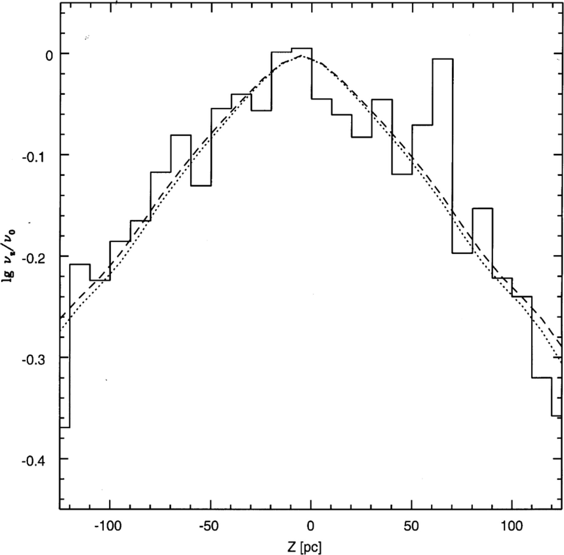
(Credit: Holmberg & Flynn 2000)
The equilibrium dynamical model does a good job of fitting the density distribution. Holmberg & Flynn (2000) find the best-fitting
It is interesting at this point to contrast the two types of analyses that we discussed in this section. In a Jeans analysis, we constrain the gravitational force from observations of the density, velocity dispersion, and their gradients at the position where we constrain the force. Thus, the Jeans equations provide constraints on the gravitational potential at the same location as the measurements. In contrast, using the full distribution function, we can use observations of the distribution function at one location, to constrain the gravitational potential over a much larger volume. Equation \(\eqref{eq-vertdens_fromfvz0}\) demonstrates that we can constrain the gravitational potential over the entire volume covered by the orbits whose velocity distribution we observe at the mid-plane. This is the case as long as we have measurements of the density throughout this volume, but we do not require kinematics throughout the volume, unlike when using the Jeans equation. Thus, using the full distribution function is more powerful than using the Jeans equation. This is generally the case.
11.4.4.2. The local surface density of matter and the local dark-matter density
When we measure the vertical density and kinematics of stars at larger distances from the Milky-Way mid-plane (\(z \gtrsim z_d\)), the gravitational force (e.g., determined using the vertical Jeans equation) most directly measures the surface density because of Equation \(\eqref{eq-surfdens-frompoisson}\). If we can measure how the surface density depends on height from \(z \approx z_d \approx 300\,\mathrm{pc}\) to \(z \gtrsim 1\,\mathrm{kpc}\), we can decompose the surface density into the contribution from the disk and that from the dark-matter halo. This is because the contribution from the disk saturates at \(z \gtrsim z_d\). The contribution to the density from the dark-matter halo is roughly constant (because the halo density only has gradients on scales \(\approx R \gg z_d\) near the Sun) and therefore provides a constant increase of \(\Sigma(z;R)\). Thus, in a simple model of a vertically-exponential disk plus a constant-density dark matter halo, the surface density is
where \(\Sigma_d(R)\) is the total surface density of the disk at radius \(R\) and \(\rho_\mathrm{DM}(R)\) is the local dark-matter density. Measurements of the density and kinematics of stars between \(z_d \lesssim z \lesssim \mathrm{few}\times z_d\) can therefore constrain the main parameters of this simple model: \(\Sigma_d(R)\), \(z_d\), and \(\rho_\mathrm{DM}(R)\).
A pioneering analysis of this type was done by Kuijken & Gilmore (1989a). They determined the density and kinematics of a sample of K dwarfs toward the South Galactic Pole and fit it by predicting the velocity distribution from the observed density distribution using Equation \(\eqref{eq-verticaldf-fordens}\) for different potentials. They predict the full velocity distribution, use it to compute the probability of the data for different models of the potential, and maximize the probability to find the best potential. However, to compare their fit to the data, it is useful to determine the moments of the velocity distribution, both for the data and the model. This comparison is shown in their Figure 13:
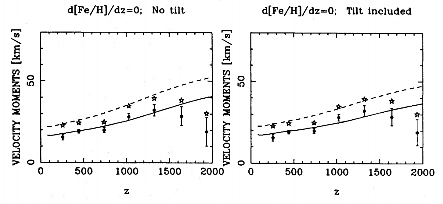
(Credit: Kuijken & Gilmore 1989a)
The sold line and dots are the first moment of the velocity distribution (the first moment here is that of \(|v_z|\) rather than \(v_z\), because the latter is zero for an equilibrium disk that is symmetric around the mid-plane), while the dashed line and stars are the square root of the second moment (the velocity dispersion). The left-hand panel is for a model where they set the tilt of the velocity ellipsoid to zero in their model, while in the right-hand panel the model assumes the maximal tilt (see above). It is clear that the tilt has only a small effect on the model.
Because their data set was small, Kuijken & Gilmore (1989a) added an additional constraint to their model to also match the rotation curve using the same disk-plus-halo model that they used (this constraint goes beyond using the slope of the rotation curve to determine the phantom density in Equation \([\ref{eq-phantomdens-oort}]\)). Because their data was mostly around \(z \approx 1.1\,\mathrm{kpc}\), they found that they could not unambiguously decompose \(\Sigma(z;R)\) into the disk and halo components (like in Equation \(\ref{eq-surfdens-decompose-disk-halo}\), but they used a different model decomposition), but instead best measured the surface density at the typical height of their sample: \(\Sigma(z=1.1\,\mathrm{kpc};R)\) (as expected from Equation \(\ref{eq-surfdens-frompoisson}\)). For this they found (Kuijken & Gilmore 1991):
This is still often used as a constraint on the local mass distribution, even though it has been refined by more recent analyses. Because they could not unambiguously decompose the surface density into disk and halo, they did not directly measure \(\rho_\mathrm{DM}(R_0)\) .
Because stars at large distances \(z \approx 1\,\mathrm{kpc}\) with accurate distances and velocities are required to measure \(\Sigma(z;R)\) from the vertical dynamics, for a long time the Kuijken & Gilmore (1989a) constraint remained the best measurement. This has changed during the last decade, due to the appearance of large spectroscopic surveys that contain large samples of disk stars around \(z \approx 1\,\mathrm{kpc}\) for which accurate distances can be obtained from the precise photometry provided by large photometric surveys (e.g., SDSS/SEGUE; Yanny et al. 2009). Better measurements of the dark-matter density can be obtained by observing the kinematics of stars at \(z \gtrsim 1.5\,\mathrm{kpc}\), because at these heights the only increase in the surface density comes from the dark-matter density (the disk density is essentially zero at such large heights above the mid-plane). However, such measurements are difficult to obtain. An analysis of this type was performed by Bovy & Tremaine (2012), who used measurements of the kinematics of red giants from Moni Bidin et al. (2012) to determine \(\Sigma(z;R_0)\) at \(1.5\,\mathrm{kpc}\gtrsim z \gtrsim 4.5\,\mathrm{kpc}\) using the Jeans Equation \(\eqref{eq-jeans-vertical-force}\) including the tilt term (which was also measured from the kinematics), assuming \(\nu(z) \propto e^{-|z|/[900\,\mathrm{pc}]}\) because the density was not directly measured (this assumption only has s small effect on the results, because the scale height realistically cannot be much larger or smaller than 900 pc). The measured \(\Sigma(z;R)\) clearly displays the expected linear trend with height expected if the only contribution to the density is a constant dark-matter halo density:
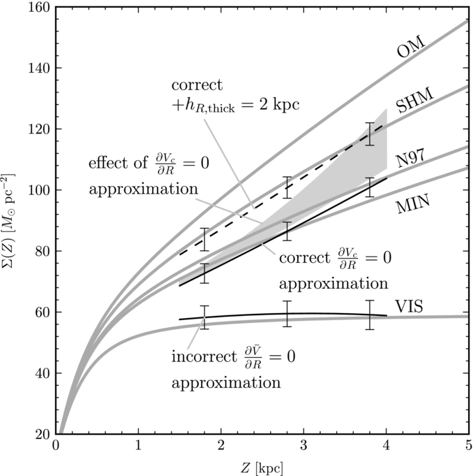
(Credit: Bovy & Tremaine 2012)
The solid line with error bars is the main result (the lower solid line labeled as “incorrect” shows the result of making an incorrect assumption about the asymmetric drift, which was made in the original analysis of these data). The linear slope gives a measurement of the local dark matter density of
At the time, this was the first high-confidence determination of the local dark-matter density.
In this section, we have focused on analyses that either assume that the vertical kinematics is decoupled from the planar kinematics or take into account the coupling using the tilt term in the vertical Jeans equation. More sophisticated analyses have been performed by Bovy & Rix (2013) (of the SDSS/SEGUE data) and Piffl et al. (2014) (of RAVE data; Steinmetz et al. 2006). These papers use equilibrium distribution models that are functions of three integrals of the motion (called the actions) and these models properly take into account the coupling between the vertical and planar motions. Further information on these types of models can be found in Binney (2010), Binney & McMillan (2011), and Binney (2012b).