
19. ⚠️🚧 Numerical methods 🚧🚨
Much of galactic dynamics research is performed numerically, but so far we have largely discussed (parts of) areas of the subject that can be solved analytically, or at most with some simple numerical integration. The one exception is numerical orbit integration, which we have used to provide example orbits throughout the previous chapters, but we have not yet discussed in detail how this orbit integration is achieved. We fill in this gap in this chapter and give an overview of the main methods of numerical galactic dynamics.
Stellar and galactic dynamics is split into two qualitatively different regimes: collisional vs. collisionless collisional (see Chapter 6.1). In the collisional regime (e.g., for stellar clusters), interactions between individual bodies are important to the evolution of the stellar system. In the collisionless regime (e.g., stars orbiting in galaxies), the density field is to an excellent approximation smooth and individual encounters can be ignored. By and large, stellar systems can be unambiguously assigned to one of these two regimes based on the estimated relation time \(t_\mathrm{relax} \approx t_\mathrm{cross}\,N/[8\,\ln N]\) (see Chapter 6.1). When \(t_\mathrm{relax} \lesssim t_H\), the Hubble time (\(t_H = 1/H \approx\) the age of the Universe, where \(H\) is the Hubble constant), as is the case for globular clusters (or for that matter, the solar system), then the system is collisional; when \(t_\mathrm{relax} \gg t_H\), as is the case for all galaxies, then the system is collisionless. However, there can be dynamical situations that straddle the boundary of the collisional/collisionless regimes. For example, the evolution of globular clusters in their host galaxy might require a combination of collisional dynamics for the internal dynamics, and collisionless dynamics, for the host galaxy. Another example is the effect of giant molecular clouds (GMCs) on stellar disks: the stellar disk itself is collisionless, but collisions between stars and GMCs have a large effect on timescales \(\approx t_H\). Situations where collisionless and collisional dynamics both play a role require special care.
Even though the numerical techniques used to simulate collisional and collisionless systems are similar, they derive from qualitatively different equations and this is important to keep in mind. To investigate the dynamics of a collisional system of \(N\) particles requires following the full \(6N\) dimensional phase-space \((\vec{w}_1,\vec{w}_2,\ldots,\vec{w}_N)\), where \(\vec{w}_i = (\vec{q}_i,\vec{p}_i)\) is the six-dimensional phase-space position of particle \(i\) as in Chapter 6.3, where we now explicitly use the momentum \(\vec{p}_i = m_i\,\vec{v}_i\), with \(m_i\) the mass. A straightforward way to do this is to evolve the system of \(N\) particles with masses \(m_i\) in its Hamiltonian
by solving the \(6N\) Hamilton’s equations for this system: \(\forall i\)
The main numerical difficulties in solving this equation for a large number of particles are (a) the calculation of the mutual forces of all \(N\) particles in the right-hand side of Equation \(\eqref{eq-collisional-Heq-2}\) and (b) the efficient numerical solution of the ordinary differential Equations \(\eqref{eq-collisional-Heq-1}\) and \(\eqref{eq-collisional-Heq-2}\).
As we discussed in Chapter 6.3, for collisionless systems made up of \(N\) particles we do not need to track the full \(6N\) dimensional phase-space distribution function \(f^{(N)}(\vec{w}_1,\vec{w}_2,\ldots,\vec{w}_N,t)\), but rather only require the six-dimensional distribution function \(f(\vec{w},t)\). And a good thing this is the case, because otherwise we could not hope to study the dynamics of dark-matter halos that in all likelihood consist of at least a trillion trillion trillion trillion particles. The distribution function \(f(\vec{w},t)\) satisfies the collisionless Boltzmann equation (Equation 6.30)
Thus, to determine the evolution of a collisionless system from an initial condition \(f(\vec{w},t=0)\)—which could be an initial pattern of density fluctuations soon after the Big Bang for a cosmological simulation—we need to solve a partial differential equation for the evolution of \(f(\vec{w},t)\), not a set of ordinary differential equations for the phase-space positions \((\vec{w}_1,\vec{w}_2,\ldots,\vec{w}_N)\) like for a collisional system.
Even though the evolution equations that need to be solved for a collisional and a collisionless system are quite different, it turns out that the solution of both—as we discuss further in Section 19.3 below—requires the same basic steps: (a) determining the mutual gravitational forces for a system of \(N\) bodies and (b) integrating Hamilton’s equations for the motion of a body in a gravitational potential. We discuss numerical methods for these two ingredients, which have wider applicability in galactic dynamics, first and then return to the question of how to solve the full collisional or collisionless evolution of a stellar system.
19.1. Poisson \(N\)-body solvers
In the previous chapters, we have extensively discussed the solution of the Poisson equation for spherical, disky, and triaxial mass distributions. We have derived expressions that can be used to compute the gravitational potential of a spherical mass distribution in Chapter 3.2, of a razor-thin disk in Chapter 8.3.2, a thick disk in Chapter 8.3.4, and for a triaxial mass distribution that is stratified on similar ellipsoids in Chapter 13.2.2. While these are fairly general expressions, they only apply in situations of relatively high symmetry and they do not solve the Poisson equation for a general density \(\rho(\vec{x})\). In this section, we discuss general methods using in N-body simulations for solving the Poisson equation for a given density \(\rho(\vec{x})\); we refer to these methods as Poisson solvers. In one of the advanced-topics chapters, we discuss basis-function-expansion techniques for solving the Poisson equation.
\(N\)-body simulations, whether collisional or collisionless, use individual particles to represent the stellar system under investigation. A common problem to all \(N\)-body methods is computing the gravitational potential corresponding to \(N\) particles. Methods to do this are called \(N\)-body (Poisson) solvers.
The gravitational potential for a set of \(N\) point-like particles at positions \(\vec{x}_i\) and with masses \(m_i\) is given by
For a particle \(j\) at \(\vec{x}_j\) that is part of the \(N\) particles, the potential is given by summing the contributions from the other particles
To compute the gravitational potential for all \(N\) particles using this equation naively requires \(\mathcal{O}(N^2)\) operations, \(\mathcal{O}(N)\) per particle. Various methods have been designed to overcome this computational burden to allow simulations that these days can involve up to \(N\approx 10^{10}\) particles.
In collisionless \(N\)-body simulations the particles are used as convenient tracers of the smooth density field (see the start of this chapter and below). When two particles approach each other, the potential diverges, because \(1/|\vec{x}_j-\vec{x}_i| \rightarrow \infty\). This divergence when using Equation \(\eqref{eq-pot-direct-sum-particles}\) is unphysical: it results from our choice to represent a smooth density field using a discrete number of particles with point-mass potentials \(\Phi(r) \propto 1/r\). A standard method for dealing with this in collisionless simulations is to introduce gravitational softening by replacing the \(\Phi(r) \propto -1/r\) behavior of the point-mass approximation with a smoother kernel \(S(r)\) that does not diverge as \(r\rightarrow 0\). Equation \(\eqref{eq-pot-direct-sum-particles}\) in that case becomes
When \(S(r) = -1/r\), this equation reduces to the point-mass limit of Equation \(\eqref{eq-pot-direct-sum-particles-softened}\). A common choice for \(S(r)\) is the potential of a Plummer sphere (see Chapter 3.4.3) with Plummer scale length \(\varepsilon\)
The parameter \(\varepsilon\) is the softening length. At separations \(\gg \varepsilon\) the softening kernel approximately reduces to the point-mass kernel, \(S(r;\varepsilon) \approx 1/r\), and the influence of softening is neglibgible. This sets the resolution of the simulation. Various other, and better, choices for the softening kernel exist; we do not discuss these here in further detail.
Simulations of galaxy dynamics often involve situations where the physical volume of the system is not well known a priori (e.g., when simulating the merger between two galaxies it is difficult to know the volume that the trajectories of the particles will occupy ahead of time). For this reason, methods that do not require prior knowledge of the system’s evolution, but rather can adapt during the simulation are generally preferred. We will discuss the main tree-based algorithm for this in some detail. Other situations, such as simulating the evolution of an individual, isolated galaxy (for example, a disk without external perturbations) or the large-scale cluster of matter in the Universe are well-behaved in the volume that they occupy and are therefore more suited to a grid-based approach or a hybrid tree-grid approach. We will not discuss these approaches in detail here.
19.1.1. Direct summation
The simplest, and adaptive, manner for computing the potential and gravitational forces for all \(N\) particles in an \(N\)-body simulation is direct summation. That is, we compute the potential directly from Equation \(\eqref{eq-pot-direct-sum-particles}\); the force is given by a similar sum
As discussed above, computing the gravitational force for all \(N\) particles requires \(\mathcal{O}(N^2)\) operations. This scaling means that it is in practice difficult to run simulations with large numbers of particles using direct summation. Despite the adverse scaling, direct summation has several advantages:
Direct summation is straightforward to implement: The equations for the potential and the force involve only a small number of elementary mathematical functions and operations. Thus, it is easy to code up the direct summation formula in a few lines of code in any programming language. Moreover, the operations involved in direct summation are typically highly optimized in the programming language itself, such that you will get quite good performance with a simple implementation (for example, the implementation in
numpybelow allows us to compute the potential for \(N=5000\) particles in \(\approx 1\,\mathrm{s}\), which was the state-of-the-art around 1990). This also means that significant speed-ups can be achieved by further optimizing the operations involved in direct summation, for example, on specialized hardware.Computing the forces using Equation \(\eqref{eq-force-direct-sum-particles}\) manifestly satisfies Newton’s third law and linear momentum will be conserved. This is not the case for the popular tree-based approximation described below.
The particles used in collisional simulations do represent true bodies, e.g., stars in a globular cluster or planets in a planetary system. In this case, close encounters and the non-smoothness of the gravitational potential are physical effects that need to be included in simulations of these systems. Direct summation is the only method that reliably computes the gravitational potential for a set of \(N\) collisional particles and is therefore the standard method for collisional simulations.
To illustrate direct summation, we implement a simple function using numpy (note that this is an inefficient implementation, because we compute all mutual distance twice to keep the code simple; this doesn’t change the scaling of the code with \(N\), but a better implementation would be twice as fast):
[77]:
def pot_directsum(pos):
    """
    NAME: pot_directsum
    PURPOSE: compute the gravitational potential for a set
            of particles using direct summation
            (assumes Gm=1 for all particles)
    INPUT: pos - positions of the particles [N,2]
    OUTPUT: potential at the location of each particle (array)"""
    invdist= 1./numpy.sqrt(numpy.sum((pos[:,:,None]-pos[:,:,None].T)**2.,
                                     axis=1))
    numpy.fill_diagonal(invdist,0.)
    return -numpy.sum(invdist,axis=1)
Let’s sample a set of \(N=60\) particles in two dimensions \((x,y)\) scattered around the \(y = x^3\) locus and compute the potential at the location of the 10-th particle. The particles are distributed as follows
[105]:
def sample_yx3(npos):
    numpy.random.seed(1) # Make sure we get a reproducible set
    pos= numpy.random.random((npos,2))*2.-1.
    pos[:,1]*= 0.2
    pos[:,1]+= pos[:,0]**3
    return pos
npos= 60
pindx= 10 # index of point to focus on
pos= sample_yx3(npos)
figsize(6,4)
plot(pos[:,0],pos[:,1],'o',ms=5.,zorder=2)
plot(pos[pindx,0],pos[pindx,1],'d',ms=8.,zorder=2)
xlabel(r'$x$'); ylabel(r'$y$');
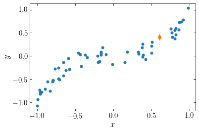
The orange diamond is the point at which we want to compute the potential. To compute the potential, we require the distance to each point, illustrated in the following figure
[109]:
figsize(6,4)
plot(pos[:,0],pos[:,1],'o',ms=5.,zorder=2)
plot(pos[pindx,0],pos[pindx,1],'d',ms=8.,zorder=2)
for ii in range(npos):
    plot([pos[ii,0],pos[pindx,0]],[pos[ii,1],pos[pindx,1]],
         '-',color='#2ca02c',lw=0.5,zorder=0)
xlabel(r'$x$'); ylabel(r'$y$');
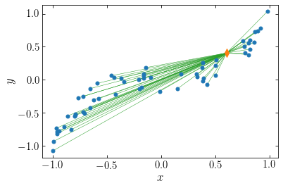
The potential at the orange point is given by
[110]:
pot_directsum(pos)[pindx]
[110]:
-106.92077175412579
Next, we can measure the time it takes to compute the gravitational potential of all \(N\) particles using our implementation, as a function of \(N\). We sample positions using the function defined above for various \(N\), compute the gravitational potential using direct summation for each sample (averaging the time to do this over five trials to lower noise in the time estimate), and plot the time vs. \(N\).
[119]:
import time
Ns= (10.**numpy.linspace(0.5,4.1,11)).astype('int')
times= numpy.empty(len(Ns))
ntrials= 5
for ii,N in enumerate(Ns):
    pos= sample_yx3(N)
    trial_times= numpy.empty(ntrials)
    for jj in range(ntrials):
        start= time.time()
        pot_directsum(pos)
        trial_times[jj]= time.time()-start
    times[ii]= numpy.median(trial_times)
loglog(Ns,times*10.**3.,'o-',lw=2.)
# reference line
plot([100.,Ns[-1]],[3.,3.*(Ns[-1]/100.)**2.],'-')
xlabel(r'$N$'); ylabel(r'$\Delta t\,(m\mathrm{s})$');
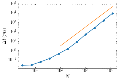
For reference, the orange line shows the \(\Delta t \propto N^2\) behavior. At small particle numbers the gravity calculation only takes a fraction of a milli-second and the overhead in the calculation dominates; therefore the time does not increase much when we increase \(N\). Once \(N \gtrsim 100\), the number of operations involved starts to dominate the behavior and the curve approaches the expected \(\Delta t \propto N^2\) behavior.
Thus, direct summation is a simple and reliable method for computing the gravitational potential for \(N\) point masses (or softened masses). However, it’s \(\mathcal{O}(N^2)\) behavior means that large, collisionless simulations cannot be performed using direct summation. Because the \(N\) particles for collisionless systems only approximate the density field, we can use approximate methods to calculate the gravitational potential for the \(N\) particles. As long as the error from the latter approximation is smaller than that from approximating the density using \(N\) particles in the first place, the gravity calculation will not be the limiting factor for the numerical accuracy of the simulation.
19.1.2. Tree-based solvers
Tree-based solvers use a tree structure to hierarchically group particles into localized structures. They then compute the gravitational field at any given position by grouping together particles at large distances, automatically adjusting the volumetric grouping based on the distance. The first tree-based gravity algorithm was introduced by Barnes & Hut (1986) and we describe the basics of this algorithm here.
Tree-based solvers start by hierarchically subdividing the positional data into smaller and smaller groupings. This is typically done using an oct-tree, which is constructed in the following way. The first level of the oct-tree is a single cube centered at the three-dimensional center of the data (the straight center halfway between minimum and maximum in each dimension) that encompasses the entire data set. We then sub-divide this root cube into the 8 sub-cubes, which are children of the parent cube, and assign to each sub-cube the data points that fall in this sub-cube. For each sub-cube, if it contains less than \(N_\mathrm{max}\) particles, we stop sub-dividing it, while if it has more than \(N_\mathrm{max}\) particles, we further sub-divide it into 8 further sub-cubes and repeat the same procedure. We do not track empty child sub-cubes. Thus, we end up with a hierarchical sub-division of the full data set: in low-density regions, sub-cubes will have less than \(N_\mathrm{max}\) particles at a relatively early stage in the hierarchy where the sub-cubes are relatively large, while in high-density region, the hierarchy will run much deeper and the sub-cubes will be small. Thus, the hierarchical tree automatically uses a high-resolution structure in high-density regions and a low-resolution structure in low-density regions.
The hierarchical-tree data structure clearly lends itself to being built through recursion: we implement the division into sub-cubes for the parent cube and then recursively apply it to each sub-cube (note that we say “cube” and “square” below, but if the data does not span the same width in each direction, the sides of the cube/square will not all have equal size; however you can still think of them as cubes/squares in coordinates where each axis is normalized by the span of the data in that
direction; in general we will refer to the cubes (in 3D) or squares (in 2D) as cells below). To illustrate the tree-based gravity solver, we will build a quad-tree, that is a two-dimensional version of an oct-tree, which lends itself better to visualization of the algorithm. The quad-tree has a parent square that gets divided into sub-squares in direct analogy to the cubes of the oct-tree. We will present a full QuadTree class later that both builds the tree and uses it to compute
the gravitational force, but we start by setting up the basic hierarchical structure of the tree.
[151]:
class QuadTree:
    """QuadTree: a 2D version of a gravitational OctTree;
        partially inspired by astroML's QuadTree
        (http://www.astroml.org/book_figures/chapter2/fig_quadtree_example.html)"""
    def __init__(self,pos,dmin=None,dmax=None,nmax=1):
        """
        NAME:   __init__
        PURPOSE: initialize a QuadTree, assumes equal masses
        INPUT:
            pos - data positions [N,2]
            dmin= (None) lower edge in [x,y]
            dmax= (None) upper edge in [x,y]
            nmax= (1) maximum number of points / leaf
        """
        self.pos= pos
        if dmin is None: self.dmin= numpy.amin(self.pos,axis=0)
        else: self.dmin= dmin
        if dmax is None: self.dmax= numpy.amax(self.pos,axis=0)
        else: self.dmax= dmax
        self.width= self.dmax-self.dmin
        self.midpoint= 0.5*(self.dmin+self.dmax)
        # Build child nodes
        self.children= []
        if len(self.pos) > nmax:
            compares= [1,-1]
            new_dmins= numpy.array([self.dmin,self.midpoint]).T
            new_dmaxs= numpy.array([self.midpoint,self.dmax]).T
            for ii in range(2):
                for jj in range(2):
                    tindx= (compares[ii]*self.pos[:,0]
                            < compares[ii]*self.midpoint[0])\
                        *(compares[jj]*self.pos[:,1]
                          < compares[jj]*self.midpoint[1])
                    if numpy.sum(tindx) > 0:
                        self.children.append(QuadTree(\
                          self.pos[tindx],nmax=nmax,
                          dmin=numpy.array([new_dmins[0,(1-compares[ii])//2],
                                            new_dmins[1,(1-compares[jj])//2]]),
                          dmax=numpy.array([new_dmaxs[0,(1-compares[ii])//2],
                                            new_dmaxs[1,(1-compares[jj])//2]])))

    def draw(self,ax):
        """
        NAME: draw
        PURPOSE: Recursively plot the populated parts of the tree
        INPUT:
            ax - matplotlib axis object to plot on
        """
        if len(self.children) == 0:
            rect= Rectangle(self.dmin,*self.width, zorder=0,
                            ec='k',fc='none')
            ax.add_patch(rect)
        else:
            for child in self.children:
                child.draw(ax)
        return None
The QuadTree object creates the parent square, centering it on the data, and then builds a list of child sub-squares, by going through the eight possible sub-squares. Each child is instantiated as another QuadTree object, with the appropriate lower and upper boundaries for the sub-square. This procedure then automatically recurses until the bottom of the hierarchy is reached. We have included a simple function to draw the populated (sub-)squares of the tree.
We can apply this hierarchical-tree algorithm to the data set for which we obtained the gravitational potential through direct summation in the previous section. Let’s run the algorithm with \(N_\mathrm{max} = 5\). This gives the following division of the data
[153]:
npos= 60
pos= sample_yx3(npos)
QTree= QuadTree(pos,nmax=5)
figsize(6,4)
plot(pos[:,0],pos[:,1],'o',ms=5.,zorder=2)
QTree.draw(gca())
xlabel(r'$x$'); ylabel(r'$y$');
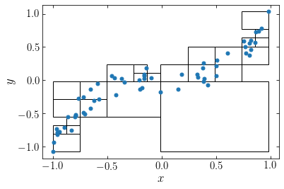
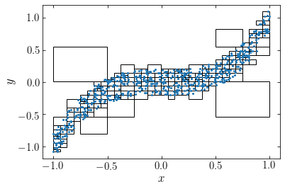
We see that the tree extends down four levels in the hierarchy in the high-density regions. If we instead apply the algorithm to \(N=600\) particles sampled from the same distribution, we see that the automatically places a high-resolution grid around the high-density region:
[154]:
npos= 600
pos= sample_yx3(npos)
QTree= QuadTree(pos,nmax=5)
figsize(6,4)
plot(pos[:,0],pos[:,1],'o',ms=2.,zorder=2)
QTree.draw(gca())
xlabel(r'$x$'); ylabel(r'$y$');
We can then use the tree to simplify the gravity calculation by approximating distance cells as a unit. This approximation is typically performed using a limiting opening angle \(\theta_\mathrm{lim}\). For this we compute the weighted mean \(\bar{\vec{x}}_{\mathcal{C}}\) for each cell \(\mathcal{C}\) during the tree-building phase and the cell’s size \(S_{\mathcal{C}} = \mathrm{max}_{i\in \mathcal{C}} |\vec{x}_i-\bar{\vec{x}}_{\mathcal{C}}|\), where
For a distant point \(\vec{x}_j\) we then compute the opening angle \(\theta_{j\mathcal{C}}\) of cell \(\mathcal{C}\) as seen by point \(\vec{x}_j\): \(\theta_{j\mathcal{C}} = S_{\mathcal{C}} / |\vec{x}_j-\bar{\vec{x}_{\mathcal{C}}}|\), that is, as size divided by distance (in the small-angle approximation). This is an approximate opening angle, because the rectangular cell does not appear as a circle, but from the definition of the width the circle with radius \(\theta_{j\mathcal{C}}\) always encompasses the cell, which is necessary for the approximation to be well-behaved. We then approximate the cell as a single unit if \(\theta_{j\mathcal{C}} < \theta_{\mathrm{lim}}\) and refer to it below as a single-unit cell.
To compute the gravity for a given point \(\vec{x}_j\) we then proceed down the tree as follows (we assume that \(\vec{x}_j\) is part of the \(N\) particles and therefore inside the parent cube). For each of the populated children \(\mathcal{C}\) of the parent cube we compute \(\theta_{j\mathcal{C}}\). If for cell \(\mathcal{C}\) we have that \(\theta_{j\mathcal{C}} < \theta_{\mathrm{lim}}\), we approximate that cell as a single unit from the perspective of point \(\vec{x}_j\) and do not consider the children of \(\mathcal{C}\). If we have that \(\theta_{j\mathcal{C}} \geq \theta_{\mathrm{lim}}\), we split the cell into its (populated) children and repeat the procedure. We end up with a subset of the cells in the hierarchical tree, the single-unit cells for point \(\vec{x}_j\).
We add this functionality to our QuadTree class: in the object initialization, we add the calculation of the mean \(\bar{\vec{x}}_{\mathcal{C}}\) and the size \(S_C\) and then we add a function to draw the cells that can be approximated as a single unit for a given point \(\vec{x}_j\) and a given limiting opening angle \(\theta_\mathrm{lim}\). We also add the ability to plot the mean for each cell.
[178]:
class QuadTree:
    """QuadTree: a 2D version of a gravitational OctTree;
        partially inspired by astroML's QuadTree
        (http://www.astroml.org/book_figures/chapter2/fig_quadtree_example.html)"""
    def __init__(self,pos,dmin=None,dmax=None,nmax=1):
        """
        NAME:   __init__
        PURPOSE: initialize a QuadTree, assumes equal masses
        INPUT:
            pos - data positions [N,2]
            dmin= (None) lower edge in [x,y]
            dmax= (None) upper edge in [x,y]
            nmax= (1) maximum number of points / leaf
        """
        self.pos= pos
        if dmin is None: self.dmin= numpy.amin(self.pos,axis=0)
        else: self.dmin= dmin
        if dmax is None: self.dmax= numpy.amax(self.pos,axis=0)
        else: self.dmax= dmax
        self.width= self.dmax-self.dmin
        self.midpoint= 0.5*(self.dmin+self.dmax)
        # For multipole expansion
        self.mean= numpy.mean(self.pos,axis=0)
        self.size= numpy.amax(self.pos-self.mean)
        # Build child nodes
        self.children= []
        if len(self.pos) > nmax:
            compares= [1,-1]
            new_dmins= numpy.array([self.dmin,self.midpoint]).T
            new_dmaxs= numpy.array([self.midpoint,self.dmax]).T
            for ii in range(2):
                for jj in range(2):
                    tindx= (compares[ii]*self.pos[:,0]
                            < compares[ii]*self.midpoint[0])\
                        *(compares[jj]*self.pos[:,1]
                          < compares[jj]*self.midpoint[1])
                    if numpy.sum(tindx) > 0:
                        self.children.append(QuadTree(\
                          self.pos[tindx],nmax=nmax,
                          dmin=numpy.array([new_dmins[0,(1-compares[ii])//2],
                                            new_dmins[1,(1-compares[jj])//2]]),
                          dmax=numpy.array([new_dmaxs[0,(1-compares[ii])//2],
                                            new_dmaxs[1,(1-compares[jj])//2]])))

    def draw(self,ax,show_mean=True):
        """
        NAME: draw
        PURPOSE: Recursively plot the populated parts of the tree
        INPUT:
            ax - matplotlib axis object to plot on
            show_mean= (True) if True, also plot the mean of th cell
        """
        if len(self.children) == 0:
            rect= Rectangle(self.dmin,*self.width, zorder=0,
                            ec='k',fc='none')
            ax.add_patch(rect)
            if show_mean:
                plot(self.mean[0],self.mean[1],'s',color='#d62728',zorder=1)
        else:
            for child in self.children:
                child.draw(ax,show_mean=show_mean)
        return None

    def draw_active(self,newpos,theta_lim,ax,show_mean=True,connect_mean=False):
        """
        NAME: draw_active
        PURPOSE: Recursively plot the active areas of the tree
            for a given point, that is, cells included in the
            gravity calculation
        INPUT:
            newpos - position at which to compute the potential
            theta_lim - maximum opening angle in rad
            ax - matplotlib axis object to plot on
            show_mean= (True) if True, also plot the mean of the cell
            connect_mean= (False) if True, also connect the mean and the position
        """
        ang= self.size/numpy.linalg.norm(newpos-self.mean)
        if len(self.children) == 0 or ang < theta_lim:
            rect= Rectangle(self.dmin,*self.width, zorder=0,
                            ec='#9467bd',fc='none')
            ax.add_patch(rect)
            if show_mean:
                plot(self.mean[0],self.mean[1],'s',color='#d62728',zorder=1)
            if connect_mean:
                plot([newpos[0],self.mean[0]],
                     [newpos[1],self.mean[1]],
                     '-',color='#2ca02c',lw=0.5,zorder=0)
        else:
            for child in self.children:
                child.draw_active(newpos,theta_lim,ax,
                                  show_mean=show_mean,connect_mean=connect_mean)
        return None
To illustrate this procedure, we return to our \(N=60\) example from the direct-summation section and plot the single-unit cells for \(\theta_\mathrm{lim} = 0.5\) for the tenth point (the point for which we illustrated the direct-summation approach above)
[179]:
npos= 60
pos= sample_yx3(npos)
pindx= 10
QTree= QuadTree(pos,nmax=5)
figsize(6,4)
plot(pos[:,0],pos[:,1],'o',ms=5.,zorder=2)
plot(pos[pindx,0],pos[pindx,1],'d',ms=8.,zorder=2)
QTree.draw_active(pos[pindx],.5,gca(),show_mean=False)
xlabel(r'$x$'); ylabel(r'$y$');
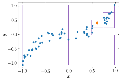
The single-unit cells are shown as purple rectangles and the point of interest is the orange diamond. We see that particles that are far from the point of interest can be approximated as a single large cell, high-up in the tree hierarchy, while nearby particles need to be grouped in smaller cells. The set of single-unit cells for a given point is not the same as the bottom layer of the tree hierarchy, which we displayed above.
This single-unit-cell mapping also depends on the point of interest. If instead of looking at point 10, we look at point 30, we get the following single-unit cells:
[180]:
npos= 60
pos= sample_yx3(npos)
pindx= 30
QTree= QuadTree(pos,nmax=5)
figsize(6,4)
plot(pos[:,0],pos[:,1],'o',ms=5.,zorder=2)
plot(pos[pindx,0],pos[pindx,1],'d',ms=8.,zorder=2)
QTree.draw_active(pos[pindx],.5,gca(),show_mean=False)
xlabel(r'$x$'); ylabel(r'$y$');
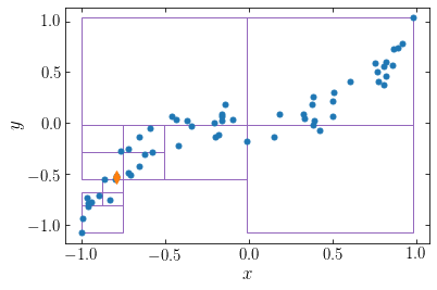
The point of interest is now at the lower left of the distribution and particles near the top, right can bow be grouped in large single-unit cells, while the particles at the lower left need to be grouped in smaller cells.
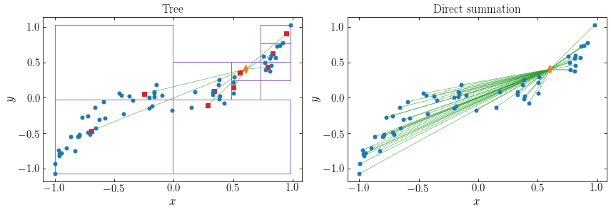
The approximation means that we can compute the gravity based on a much smaller number of particle–cell interactions compared to the \(N\) particle–particle interactions for direct summation. We can illustrate that by displaying the means of the single-unit cells, connecting the point of interest to this, and juxtaposing this to the direct-summation graph from above. For point 10:
[185]:
npos= 60
pos= sample_yx3(npos)
pindx= 10
QTree= QuadTree(pos,nmax=5)
figsize(12,4)
subplot(1,2,1)
plot(pos[:,0],pos[:,1],'o',ms=5.,zorder=2)
plot(pos[pindx,0],pos[pindx,1],'d',ms=8.,zorder=2)
QTree.draw_active(pos[pindx],.5,gca(),connect_mean=True)
xlabel(r'$x$'); ylabel(r'$y$')
annotate(r'$\mathrm{Tree}$',(0.5,1.075),xycoords='axes fraction',
         horizontalalignment='center',
         verticalalignment='top',size=17.)
subplot(1,2,2)
plot(pos[:,0],pos[:,1],'o',ms=5.,zorder=2)
plot(pos[pindx,0],pos[pindx,1],'d',ms=8.,zorder=2)
for ii in range(npos):
    plot([pos[ii,0],pos[pindx,0]],[pos[ii,1],pos[pindx,1]],
         '-',color='#2ca02c',lw=0.5,zorder=0)
xlabel(r'$x$'); ylabel(r'$y$');
annotate(r'$\mathrm{Direct\ summation}$',(0.5,1.075),xycoords='axes fraction',
         horizontalalignment='center',
         verticalalignment='top',size=17.)
tight_layout()
and for point 30
[186]:
npos= 60
pos= sample_yx3(npos)
pindx= 30
QTree= QuadTree(pos,nmax=5)
figsize(12,4)
subplot(1,2,1)
plot(pos[:,0],pos[:,1],'o',ms=5.,zorder=2)
plot(pos[pindx,0],pos[pindx,1],'d',ms=8.,zorder=2)
QTree.draw_active(pos[pindx],.5,gca(),connect_mean=True)
xlabel(r'$x$'); ylabel(r'$y$')
annotate(r'$\mathrm{Tree}$',(0.5,1.075),xycoords='axes fraction',
         horizontalalignment='center',
         verticalalignment='top',size=17.)
subplot(1,2,2)
plot(pos[:,0],pos[:,1],'o',ms=5.,zorder=2)
plot(pos[pindx,0],pos[pindx,1],'d',ms=8.,zorder=2)
for ii in range(npos):
    plot([pos[ii,0],pos[pindx,0]],[pos[ii,1],pos[pindx,1]],
         '-',color='#2ca02c',lw=0.5,zorder=0)
xlabel(r'$x$'); ylabel(r'$y$');
annotate(r'$\mathrm{Direct\ summation}$',(0.5,1.075),xycoords='axes fraction',
         horizontalalignment='center',
         verticalalignment='top',size=17.)
tight_layout()
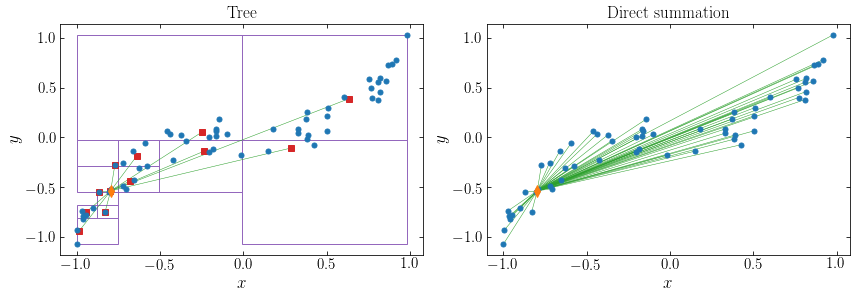
The final piece of the puzzle is how we should calculate the gravitational potential or force from the single-unit cells on a particle at position \(\vec{x}_j\). The lowest-order approximation is to approximate the single-unit cell \(\mathcal{C}\) as if all of its mass, \(M_{\mathcal{C}} = \sum_{i\in \mathcal{C}} m_i\), were concentrated in its center of mass position \(\bar{\vec{x}}_{\mathcal{C}}\). The gravitational potential at \(\vec{x}_j\) from cell \(\mathcal{C}\) is then given by
where \(S(\cdot)\) is the softening kernel.
We can go beyond this lowest-order approximation, by considering moments of the mass distribution within each cell \(\mathcal{C}\). To do this, we follow the discussion in Dehnen & Read (2011). To simplify the expressions (and to write the expressions in a general way that applies to both the 2D case that we implement below and to the 3D case), we use multi-index notation: in 3D, for integer vectors \(\vec{n} = (n_x,n_y,n_z)\), we define
The direct-summation contribution to the potential at \(\vec{x}_j\) from all particles at \(\vec{x}_i\) in \(\mathcal{C}\) is given by
We can then Taylor-expand the kernel function \(S(|\vec{x}_j-\vec{x}_i|)\) around the cell’s center of mass
and substitute this into Equation \(\eqref{eq-treegrav-directsumcell}\). Exchanging the order of the sums, we can write this as
The quantity in square brackets does not depend on \(\vec{x}_j\) and corresponds to the multipole moments \(M_{\vec{n}}(\bar{\vec{x}}_{\mathcal{C}})\) of the mass distribution in cell \(\mathcal{C}\)
In terms of the multipole moments, the potential approximation in Equation \(\eqref{eq-treegrav-multipole-approx-premultipoledef}\) becomes
The zero-th multipole is simply the mass in the cell, \(M_0(\bar{\vec{x}}_{\mathcal{C}}) = M_{\mathcal{C}}\). The zero-th order approximation version of Equation \(\eqref{eq-treegrav-multipole-approx}\) therefore reduces to Equation \(\eqref{eq-treegrav-zeroth-approx}\), as expected. Because we have defined the expansion around the center of mass, the first-order multipole moments of each cell vanish, that is \(M_{\vec{n}}(\bar{\vec{x}}_{\mathcal{C}}) = 0\) when \(|\vec{n}| = 1\). Thus, the first-order approximation is also given by Equation \(\eqref{eq-treegrav-zeroth-approx}\) and this expression is therefore accurate to first order. To go to second order and beyond requires the derivatives \(\vec{\nabla}^{\vec{n}}\,S(r)\) of the softening kernel, which quickly become complicated.
When going beyond first order multipoles, computing the multipole moments for the larger cells can involve a large subset of the particles. However, the multipole moments for a parent cell \(\mathrm{P}\) can be computed from those of its children \(\mathcal{C}\) using the shift formula for multipole moments
because then we have that
(Note that to not overburden the notation, we have left implicit whether a given multipole moment \(M_{\vec{n}}(\cdot)\) corresponds to that of the parent or the child, but it should be clear from the context which is which). Using this shift formula, we can compute the multipole moments for each cell in approximately the same number of operations.
Finally, we need to handle the case where a single-unit cell is at the bottom of the hierarchy. If the opening angle \(\theta_{j\mathcal{C}}\) is smaller than \(\theta_{\mathrm{lim}}\) we follow the procedure in terms of the multipole moments. If the opening angle is still larger than \(\theta_\mathrm{lim}\), we simply compute the potential using direct summation over the members of the cell, of which there are fewer than \(N_\mathrm{max}\) (note that if \(N_\mathrm{max}\) is one or a few, always doing direct summation at the deepest hierarchical level may be faster than using multipoles). Once we have expressions for the potential, we can obtain expressions for the force from the derivative of the potential.
We can now finalize our QuadTree class by including the calculation of the multipoles in the cell initialization (using the shift formula for parent cells), the derivatives of the kernel (using the unsmoothed point-mass kernel \(S(r) = -1/r\)), and adding a function that computes the potential at a given point \(\vec{x}_j\):
[189]:
class QuadTree:
    """QuadTree: a 2D version of a gravitational OctTree;
        partially inspired by astroML's QuadTree
        (http://www.astroml.org/book_figures/chapter2/fig_quadtree_example.html)"""
    def __init__(self,pos,dmin=None,dmax=None,nmax=1,mmax=2):
        """
        NAME:   __init__
        PURPOSE: initialize a QuadTree, assumes equal masses
        INPUT:
            pos - data positions [N,2]
            dmin= (None) lower edge in [x,y]
            dmax= (None) upper edge in [x,y]
            nmax= (1) maximum number of points / leaf
            mmax= (2; <=2) maximum multipole order to consider
        """
        self.pos= pos
        if dmin is None: self.dmin= numpy.amin(self.pos,axis=0)
        else: self.dmin= dmin
        if dmax is None: self.dmax= numpy.amax(self.pos,axis=0)
        else: self.dmax= dmax
        self.width= self.dmax-self.dmin
        self.midpoint= 0.5*(self.dmin+self.dmax)
        # For multipole expansion
        self.mean= numpy.mean(self.pos,axis=0)
        self.size= numpy.amax(self.pos-self.mean)
        if mmax > 2:
            raise NotImplementedError("Multipoles higher than 2 are not supported")
        self.ms= numpy.arange(mmax+1,dtype='int') # we only go to ms[-1]-th order
        self.multipoles= numpy.zeros((len(self.ms),len(self.ms)))
        # Build child nodes
        self.children= []
        if len(self.pos) > nmax:
            compares= [1,-1]
            new_dmins= numpy.array([self.dmin,self.midpoint]).T
            new_dmaxs= numpy.array([self.midpoint,self.dmax]).T
            for ii in range(2):
                for jj in range(2):
                    tindx= (compares[ii]*self.pos[:,0]
                            < compares[ii]*self.midpoint[0])\
                        *(compares[jj]*self.pos[:,1]
                          < compares[jj]*self.midpoint[1])
                    if numpy.sum(tindx) > 0:
                        self.children.append(QuadTree(\
                          self.pos[tindx],nmax=nmax,mmax=mmax,
                          dmin=numpy.array([new_dmins[0,(1-compares[ii])//2],
                                            new_dmins[1,(1-compares[jj])//2]]),
                          dmax=numpy.array([new_dmaxs[0,(1-compares[ii])//2],
                                            new_dmaxs[1,(1-compares[jj])//2]])))
        # Compute multipole moments
            # Obtain multipole from shifted multipoles from
            # children, upwards pass
            for child in self.children:
                offset= self.mean-child.mean
                for ii,mx in enumerate(self.ms):
                    for jj,my in enumerate(self.ms):
                        # we only go to ms[-1]-th order
                        if (mx+my) > self.ms[-1]: continue
                        for kk,mxx in enumerate(self.ms):
                            for ll,myy in enumerate(self.ms):
                                if (mxx+myy) > (mx+my): continue
                                self.multipoles[ii,jj]+=\
                                    offset[0]**mxx*offset[1]**myy\
                                    /numpy.math.factorial(mxx)\
                                    /numpy.math.factorial(myy)\
                                    *child.multipoles[ii-kk,jj-ll]
        else:
            # For leafs, directly compute multipole moments
            for ii,mx in enumerate(self.ms):
                for jj,my in enumerate(self.ms):
                    # we only go to ms[-1]-th order
                    if (mx+my) > self.ms[-1]: continue
                    self.multipoles[ii,jj]= (-1.)**(mx+my)\
                        /numpy.math.factorial(mx)/numpy.math.factorial(my)\
                        *numpy.sum((self.pos[:,0]-self.mean[0])**mx
                                   *(self.pos[:,1]-self.mean[1])**my)

    def __call__(self,newpos,theta_lim):
        """
        NAME: __call__
        PURPOSE: Recursively compute the potential for a single point
        INPUT:
            newpos - position at which to compute the potential
            theta_lim - maximum opening angle in rad
        """
        ang= self.size/numpy.linalg.norm(newpos-self.mean)
        if (len(self.children) == 0 and ang >= theta_lim) \
            or numpy.isnan(ang): # NaN when newpos *is* the current leaf
            # compute with direct summation
            dist= numpy.sqrt(numpy.sum((newpos-self.pos)**2.,axis=1))
            out= -numpy.sum(1./dist[dist > 0.])
        elif ang >= theta_lim:
            # compute from children
            out= 0.
            for child in self.children:
                out+= child(newpos,theta_lim)
        else:
            # compute from multipole moments
            out= 0.
            for ii,mx in enumerate(self.ms):
                for jj,my in enumerate(self.ms):
                    # we only go to ms[-1]-th order
                    if (mx+my) > self.ms[-1]: continue
                    out-= self.multipoles[ii,jj]\
                        *self._kernel_deriv(newpos-self.mean,ii,jj)
        return out

    def _kernel_deriv(self,pos,ii,jj):
        """The derivatives of the point-mass kernel"""
        if ii == 0 and jj == 0:
            return 1./numpy.sqrt(numpy.sum(pos**2.))
        elif ii+jj == 1:
            return 1./(numpy.sum(pos**2.))**3.*pos[0]**ii*pos[1]**jj
        elif ii == 2 or jj == 2:
            r2= numpy.sum(pos**2.)
            return 1./r2**2.5*(3.*pos[0]**(2.*ii)*pos[1]**(2*jj)-r2)
        elif ii+jj == 2:
            return 3./numpy.sum(pos**2.)**2.5*pos[0]*pos[1]

    def draw(self,ax,show_mean=True):
        """
        NAME: draw
        PURPOSE: Recursively plot the populated parts of the tree
        INPUT:
            ax - matplotlib axis object to plot on
            show_mean= (True) if True, also plot the mean of th cell
        """
        if len(self.children) == 0:
            rect= Rectangle(self.dmin,*self.width, zorder=0,
                            ec='k',fc='none')
            ax.add_patch(rect)
            if show_mean:
                plot(self.mean[0],self.mean[1],'s',color='#d62728',zorder=1)
        else:
            for child in self.children:
                child.draw(ax,show_mean=show_mean)
        return None

    def draw_active(self,newpos,theta_lim,ax,show_mean=True,connect_mean=False):
        """
        NAME: draw_active
        PURPOSE: Recursively plot the active areas of the tree
            for a given point, that is, cells included in the
            gravity calculation
        INPUT:
            newpos - position at which to compute the potential
            theta_lim - maximum opening angle in rad
            ax - matplotlib axis object to plot on
            show_mean= (True) if True, also plot the mean of the cell
            connect_mean= (False) if True, also connect the mean and the position
        """
        ang= self.size/numpy.linalg.norm(newpos-self.mean)
        if len(self.children) == 0 or ang < theta_lim:
            rect= Rectangle(self.dmin,*self.width, zorder=0,
                            ec='#9467bd',fc='none')
            ax.add_patch(rect)
            if show_mean:
                plot(self.mean[0],self.mean[1],'s',color='#d62728',zorder=1)
            if connect_mean:
                plot([newpos[0],self.mean[0]],
                     [newpos[1],self.mean[1]],
                     '-',color='#2ca02c',lw=0.5,zorder=0)
        else:
            for child in self.children:
                child.draw_active(newpos,theta_lim,ax,
                                  show_mean=show_mean,connect_mean=connect_mean)
        return None
We can now compare the tree-based calculation with \(\theta_\mathrm{lim}\) of the gravitational potential for point 10 in our \(N=60\) example with that using direct summation:
[194]:
npos= 60
pos= sample_yx3(npos)
pindx= 10
QTree= QuadTree(pos,nmax=5)
print("Tree-based potential: {0:.2f}".format(QTree(pos[pindx],0.5)))
print("Direct-summation potential: {0:.2f}".format(pot_directsum(pos)[pindx]))
Tree-based potential: -103.69
Direct-summation potential: -106.92
If we decrease \(\theta_\mathrm{lim}\), the tree-based calculation converges to the correct, direct-summation answer (the orange dashed line in the following figure):
[202]:
figsize(6,4)
theta_lims= numpy.linspace(1e-4,0.65,11)
plot(theta_lims,[QTree(pos[pindx],theta_lim) for theta_lim in theta_lims])
axhline(pot_directsum(pos)[pindx],ls='--',color='#ff7f0e')
xlim(0.75,0.)
xlabel(r'$\theta_\mathrm{lim}$')
ylabel(r'$\Phi$');
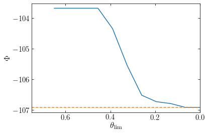
The main advantage of the tree-based algorithm over the direct-summation approach is speed: evaluating the potential or force on a given particle typically requires only \(\mathcal{O}(\ln N)\) operations (at fixed \(\theta_{\mathrm{lim}}\)) and evaluating the potential or forces for all \(N\) particles requires \(\mathcal{O}(N\,\ln N)\) operations, because each particle’s gravity calculation is performed independently from all the other gravity calculations. This \(\mathcal{O}(\ln N)\) scaling arises because when we increase the number of particles \(N\) that samples the density, the tree becomes deeper, but when computing the gravity at a given point, we only need to take the increased depth into account for the small fraction of cells with \(\theta_{j\mathcal{C}} \geq \theta_\mathrm{lim}\) (for cells with \(\theta_{j\mathcal{C}} < \theta_\mathrm{lim}\) the increased depth is ignored, because they can still be considered as a single-unit cell). For a close-to-homogeneous system with \(N=N_0\), the smallest cells in the hierarchy have linear sizes \(\propto N_0^{-1/3}\) (the inter-particle separation) and only those within a distance \(\propto N_0^{-1/3}/\theta_\mathrm{lim}\) have \(\theta_{j\mathcal{C}} \geq \theta_\mathrm{lim}\); the total number of cells with \(\theta_{j\mathcal{C}} \geq \theta_\mathrm{lim}\) is therefore \(\mathcal{O}(N_0)\). When we increase \(N\) by a factor of eight to \(8\,N_0\), the distance within which \(\theta_{j\mathcal{C}} < \theta_\mathrm{lim}\) decreases by a factor of two and therefore the volume decreases by a factor of eight; however, the size of the smallest cells similarly decreases by a factor of two, and the number of cells with \(\theta_{j\mathcal{C}} < \theta_\mathrm{lim}\) is therefore still \(\mathcal{O}(N_0)\) [not \(\mathcal{O}(N)\)]. Most of the extra work comes from dealing with these smaller cells, which adds an amount of work \(\propto N_0\). If we increase the number of particles by another factor of eight, we add again a similar amount of work. Therefore, the amount of work to compute the potential roughly increases by a constant term for each eightfold increase in the number of particles, and the total number of operations therefore scales as \(\mathcal{O}(N)\).
We can test this scaling for our example problem. The following code computes the time per force evaluation for \(N\) particles sampled from the \(y \approx x^3\) distribution above (we also track the time to setup the tree to investigate below):
[221]:
import time
Ns= (10.**numpy.linspace(0.5,5.1,11)).astype('int')
times= numpy.empty(len(Ns))
times_setup= numpy.empty(len(Ns))
ntrials= 15
for ii,N in enumerate(Ns):
    pos= sample_yx3(N)
    start= time.time()
    QTree= QuadTree(pos,nmax=5)
    times_setup[ii]= time.time()-start
    trial_times= numpy.empty(ntrials)
    for jj in range(ntrials):
        start= time.time()
        QTree(pos[0],0.5)
        trial_times[jj]= time.time()-start
    times[ii]= numpy.median(trial_times)
semilogx(Ns,times*10.**3.,'o-',lw=2.)
# reference line
plot([10.,Ns[-1]],[1.,1.*numpy.log(Ns[-1]/10.)],'-')
xlabel(r'$N$'); ylabel(r'$\Delta t/\mathrm{particle}\,(m\mathrm{s})$');
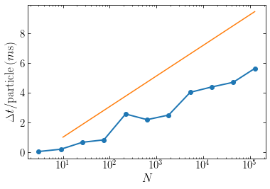
The orange line shows the slope of the expected \(\Delta t \propto \ln N\) behavior. We see that the tree-based algorithm indeed roughly scales as \(\mathcal{O}(\ln N)\).
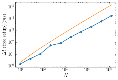
Because the size of the smallest cell is roughly equal to the inter-particle separation, which is \(\propto N^{-1/3}\), the number of layers in the tree is \(\approx \ln N^{1/3} \approx \ln N\). The total number of cells in the tree (parents and children) is therefore \(\approx N \ln N\) and because we need to do a constant amount of work to setup each cell, building the tree scales as \(\mathcal{O}(N\ln N)\).
The following figure displays the time it takes to setup the tree for our example problem as a function of \(N\). The algorithm implemented here scales close to the expected value, although seemingly somewhat closer to \(\mathcal{O}(N)\) than to \(\mathcal{O}(N\ln N)\) (the orange line is the expected \(\mathcal{O}(N\ln N)\) behavior):
[232]:
loglog(Ns[1:],times_setup[1:]*10.**3.,'o-',lw=2.)
# reference line
plot(Ns[1:],Ns[1:]*numpy.log(Ns[1:])/10.,'-')
xlabel(r'$N$'); ylabel(r'$\Delta t\ (\mathrm{tree\ setup})\,(m\mathrm{s})$');
Tree-based Poisson solvers therefore have the ability to scale to large numbers of particles.
19.2. Numerical orbit integration
For most gravitational potentials, we cannot analytically solve the equations of motion (the Kepler point-mass potential being a notable exception) or we can, but doing so is quite complicated (for example, the isochrone potential from Chapter 3.4.4). In this case, we can solve the equations of motion numerically, which we refer to as “integrating the orbit”. Newton’s second law, which we introduced in Chapter 4.1, is a ordinary differential equation (ODE)
where \(\vec{g}(\vec{x})\) is the gravitational field. The typical situation is that we have the initial position \(\vec{x}_0\) and velocity \(\vec{v}_0\) and want to find the position \(\vec{x}(t)\) and velocity \(\vec{v}(t)\) at a later time \(t\); this is an initial-value problem. As a fairly simple ordinary differential equation, Equation \(\eqref{eq-newton-second-numerical}\) can be solved using any of a large number of standard methods for finding numerical solutions of ordinary differential equations. We discuss some of these in the first subsection below.
However, in most situations in galactic dynamics, the equations of motion can be written as Hamilton’s equations using the Hamiltonian
where \((\vec{q},\vec{p})\) are the generalized coordinates and momenta–in cartesian coordinates these are simply \(\vec{q} = \vec{x}\) and \(\vec{p} = m\,\vec{v}\). As we will discuss below, we can construct better numerical orbit solutions by using and respecting the Hamiltonian structure of phase–space.
Before discussing particular algorithms, we note that not all problems in galactic dynamics are of the form described above. For example, to construct surfaces of section we want to find the position and velocity when the orbit starting at \((\vec{x}_0,\vec{v}_0)\) goes through the surface of section, which is a different problem from asking where the initial points ends up after a time \(\Delta t\) has passed. This problem can be expressed in the form above, if we re-parameterize the system such that the independent coordinate becomes a coordinate, say \(s\), that measures the distance from the surface of section such that the orbit goes through the surface of section at particular values of \(v\). The problem then has the same form as above, where \(t \rightarrow v\) and we ask where the orbit is at certain values of \(v\). We do not discuss such other problems further. Note that in Chapter 14.1, we constructed surfaces of section using a very high-time-resolution orbit integration and we found intersections numerically from the time series.
19.2.1. General ODE solvers
We write Equation \(\eqref{eq-newton-second-numerical}\) as a set of coupled, first-order (that is, only containing first-order derivatives) ordinary differential for \((\vec{x},\vec{v})\)
where we have made the possible dependence of the force on time explicit. To determine the time evolution \([\vec{x},\vec{v}](t)\) of an initial point \((\vec{x}_0,\vec{v}_0)\), we can solve this set of differential equations using any of a large number of standard techniques. To simplify the notation, we use \(\vec{w} = (\vec{x},\vec{v})\) and Equation \(\eqref{eq-newton-second-numerical-first-order-set}\) then becomes
with \(\vec{f}(\vec{w},t) = (\vec{v},\vec{g}(\vec{x},t)\). The simplest method for solving this equation is the Euler method, in which obtains the position and velocity at time \(t+\Delta t\) by moving along the derivative
The error in this method is \(\mathcal{O}([\Delta t]^2)\) and we say that this is a first-order method. In general we call a method a n-th-order method when the error is \(\mathcal{O}([\Delta t]^{n+1})\).
Euler’s method is conceptually simple—one simply takes a small step along the gradient, re-evaluates the gradient, takes a small step along the updated gradient, and so forth—but the error increases with each step and quickly becomes large, even when using a small step \(\Delta t\).
A better Euler-like approximation would be to use the derivative at the mid-way point between \(\vec{w}(t)\) and \(\vec{w}(t+\Delta t)\) to move the point \(\vec{w}(t)\). Of course, we cannot know a priori what the mid-way point is! However, we can estimate the mid-way point by doing an Euler iteration (Equation \([\ref{eq-euler-step-dt}]\)) with a step \(\Delta t\), evaluating the gradient at the estimated mid-way point, and then using this gradient to move from \(\vec{w}(t)\) to \(\vec{w}(t+\Delta t)\). This gives the following method
This method is known as the second-order Runge-Kutta method (RK2) and it is a second-order method. This method has smaller errors than the Euler method, but requires two evaluations of \(\vec{f}\left(\vec{w},t\right)\) rather than one for the Euler method. Typically, the derivative is easy enough to evaluate that the time saved by having smaller errors by far makes up for the increased time from evaluating the function twice. However, when we discuss Hamiltonian integration below, we will see that for Hamiltonian systems we can design second-order methods that only use a single evaluation of the gradient of the potential.
We can design higher-order methods by evaluating the derivatives at more than one intermediate point and/or at an estimated endpoint and combining the information from all derivatives in such a way that the total error scales as \(\mathcal{O}([\Delta t]^{n+1})\) with \(n > 2\). The most popular of such methods computes the gradient \(\vec{k}_2\) at the estimated mid-way point like for the RK2 method, but then uses this gradient to provide a different estimate for the mid-way point and computes the gradient \(\vec{k}_3\) there. This gradient is then used to estimate the endpoint, and we can compute the gradient \(\vec{k}_4\) at the estimated endpoint. Finally, the gradient at the initial point, \(\vec{k}_1\) is combined with the gradients at the intermediate points and at the endpoint to give an estimate of the endpoint that is fourth-order accurate. In detail, the method looks as follows:
The coefficients in the final line are chosen such that the error scales as \(\mathcal{O}([\Delta t]^{5})\) and this is the fourth-order Runge-Kutta (RK4) method. The fourth-order Runge-Kutta methods uses four gradient evaluations to estimate \(\vec{w}(t+\Delta t)\). The extra work from the four gradient evaluations is typically offset by the increased accuracy when integrating orbits in smooth galactic potentials.
Higher-order methods of this type can be designed by using even more mid-way estimates of the gradient; all methods become more complicated as one goes to higher order. One advantage of certain higher-order Runge-Kutta-style methods is that one can construct multiple estimates of \(\vec{w}(t+\Delta t)\) from the estimated mid-way and endpoint gradients and the difference between these values can be used to estimate the error; this error estimate can then be employed to adaptively change the step \(\Delta t\), reducing the step when the error is larger than desired. Dormand-Prince methods of fifth and eight order are popular examples of this type of method (see the Numerical Recipes book by Press et al. for more information on these).
Like for the Euler method, errors accumulate with every time step for typical orbits with Runge-Kutta (or Dormand-Prince) methods. If we use these methods to integrate orbits for many dynamical times, the total error will become large, unless one uses a prohibitively small time step. Therefore, these methods are only useful when integrating orbits for a relatively small number of dynamical times (e.g., hundreds for RK4, but it depends on the step). For \(N\)-body simulations, the gravity calculation is sufficiently slow that in practive we can only evaluate the gradient in Equation \(\eqref{eq-newton-second-numerical-first-order-set}\) once per time step. The best method that only uses a single gradient evoluation for a Hamiltonian system is not the Euler method, but a method that we will discuss next.
One situation where we have to use the methods from this section is when there are dissipative, non-gravitational forces that affect the dynamics of a star or galactic system. Examples of this include dynamical friction (which we have not yet discussed) or interactions between gravitational bodies and a gas disk (for example, in a proto-planetary disk).
19.2.2. Hamiltonian integration
The general methods for solving ordinary differential equations that we discussed in the previous section all essentially work by discretizing the differential equation. For a Hamiltonian system, we can instead discretize the Hamiltonian in a way that allows us to exactly integrate Hamilton’s equations for the discretized Hamiltonian. The advantage of such a method is that it is straightforward to discretize the Hamiltonian in such a way on long time scale, the discretized and original Hamiltonian are indistinguishable. The long-term behavior of an orbit integration will therefore remain close to the true trajectory without accumulating errors like the general ODE solvers above. We term such methods Hamiltonian integration methods.
To illustrate this, we consider the Hamiltonian in cartesian coordinates
Hamilton’s equations of motion for this Hamiltonian are
Let us now discretize the Hamiltonian by multiplying the potential in it with a Dirac comb \(\operatorname{III}(t;\Delta t)\) where
such that the discretized Hamiltonian \(H_{\Delta t}\) becomes
Using the Poisson summation formula, we can write this equivalently as
Thus, we have effectively replaced the potential with a time-dependent potential which fluctuates on timescales with periods \(T = \Delta t / j\), where \(j\) is an integer. On timescales \(\gg \Delta t\), all of these fluctuations average out and we have that \(H_{\Delta t} \approx H\). Thus, on time scales larger than the step \(\Delta t\), the difference between the discretized and the original Hamiltonian is small.
Hamilton’s equations for the discretized Hamiltonian in Equation \(\eqref{eq-hamiltonian-discretized}\) are
These equations can be solved exactly as follows, because the gradient in the second of these equations is now only non-zero at a set of discrete times \(j\,\Delta t\). Let \(j=1\). If we are at \(t=\varepsilon\), where \(\varepsilon \ll \Delta t\) is an infinitesimal number, we can integrate analytically up to \(t=\Delta t-\varepsilon\), because \(\dot{\vec{p}}\) is zero at all these times, and we thus get the update step
When we then integrate from \(\Delta t-\varepsilon\) to \(\Delta t+\varepsilon\), we can integrate Equations \(\eqref{eq-discrete-hamiltonian-qdot}\) and \(\eqref{eq-discrete-hamiltonian-pdot}\) over the time interval \(2\varepsilon\)
If we then let \(\varepsilon \rightarrow 0\), Equations \(\eqref{eq-symplectic-drift-eps}\) and Equation \(\eqref{eq-symplectic-kick-eps}\) reduce to
Thus, we first let the position move at constant momentum for a time \(\Delta t\), called the drift step, and we then update the momentum using the gradient computed at the new position, which is called the kick step. This method is similar to the Euler method from Equation \(\eqref{eq-euler-step-dt}\), except that it uses the force at the new position, rather than at the old; this method is therefore called the modified Euler method. One can show that it is also a first-order method.
Using a similar procedure, we can construct a second-order method that is widely used. Rather than starting at \(t=\varepsilon\) in the above derivation, we start at \(t=-\Delta/2\) and drift until \(t=-\varepsilon\); we then integrate over the kick from \(t=-\varepsilon\) to \(t=\epsilon\), and finally drift until \(t=\Delta t\). This also completes an increment of the system by a step \(\Delta t\); shifting all the times by \(\Delta t/2\) in this procedure (such that the step goes from \(t=0\) to \(t=\Delta t\), with the kick at \(t=\Delta t/2\)), the actual sequence of steps is
This is the drift-kick-drift leapfrog method. This is a second-order method with errors \(\mathcal{O}([\Delta t]^3)\). Like the Euler and modified Euler methods, it requires only a single force evaluation to advance the orbit by a time \(\Delta t\), but unlike the Euler methods, it is second order. A further speed-up can be achieved by chaining successive drift steps together, because the last step and the first step of the next iteration both add the same vector to the position. Therefore, as long as we do not need to know the position at the \(t=j\,\Delta t\) interval (for example, when we only record the orbit every 10 steps, we do not need to record its position for 9 out of 10 steps and we can chain the drifts for these nine steps together). For this reason, the leapfrog integrator is the preferred method for almost all collisionless simulations, which do not require high accuracy, because they use approximate forces anyway.
The main advantage of integrators that integrate an approximate Hamiltonian exactly, rather than approximately integrating the exact Hamiltonian, is that they are a legitimate phase-space mapping. Thus, Hamiltonian integration satisfies, e.g., Liouville’s theorem for the approximate Hamiltonian. As we discussed above, at timescales \(\gg \Delta t\), the exact and approximate Hamiltonian coincide. For a small enough step \(\Delta t\), this typically causes the energy error to be bounded, such that an accumulation of energy errors as for the standard ODE solvers does not occur.
Hamiltonian integrators are often called symplectic. This name comes from the fact that these integrators are Hamiltonian maps, whose mathematical structure is that of a vector flow on a symplectic manifold. Many fine dynamicists have made great contributions to the field without delving deeply into the meaning of the previous sentence and we do not discuss this further.
Most orbit integrations that one encounters in galactic dynamics can be solved using the simple leapfrog integrator above or, for test-particle orbits in a smooth gravitational field, with the fourth-order Runge-Kutta method from the previous section. Collisionless \(N\)-body simulations typically use the leapfrog method, with particles assigned to a hierarchy of step sizes \(\Delta t = \Delta T / 2^k\) that are some factor of two smaller than a maximum step size \(\Delta T\); kicks are only applied at \(\Delta t = \Delta T / 2^k\), where \(k\) can vary between different particles. This is called a block time step scheme. For further information on this scheme or on other integrators, we refer the interested reader to BT08 Sec. 3.4 or Dehnen & Read (2011).
19.3. \(N\)-body modeling
We now have all of the ingredients to come back to the problem posed at the beginning of this chapter: how to simulate the evolution of a collisional or collisionless system in time, starting from a given initial condition \((\vec{w}_1,\vec{w}_2,\ldots,\vec{w}_N,t=0)\). We first briefly discuss the collisional problem, for which we need to solve a straightforward set of equations, although the exact implementation of these equations is somewhat tricky; we won’t discuss all of the fine details about this. Then we focus for most of this section on the collisionless problem, for which the solution is less straightforward.
19.3.1. Collisional \(N\)-body modeling
As discussed at the start of this chapter, for the collisional \(N\)-body problem we need to compute orbital trajectories for the Hamiltonian of the \(N\)-particle system
Hamilton’s equations in cartesian coordinates \((\vec{x}_i,\vec{p}_i)\) for this Hamiltonian are given in Equations \(\eqref{eq-collisional-Heq-1}\) and \(\eqref{eq-collisional-Heq-2}\). Typical collisional settings are star-cluster dynamics or the gravitational dynamics of multi-planetary systems (like the solar system).
Because the \(N\) particles in a collisional simulation actually correspond to physical objects, the lore is that the gravitational potential and its derivatives needs to be computed using the direct summation approach from Section 19.1.1 above, which has an algorithmic complexity of \(\mathcal{O}(N^2)\). Thus, the gravity calculation is very expensive. This does not matter for planetary systems, where \(N = \mathcal{O}(10)\) at most (the gravity from smaller objects such as asteroids can be ignored for the motion of the other bodies in the system), but it is a prohibitive scaling for large star clusters, where \(N\) can be up to a few times \(10^6\). Nevertheless, direct summation remains the standard method for computing the potential for any collisionless system (however, see Dehnen 2014 for a method that scales better than \(\mathcal{O}[N]\)).
Once the potential is computed using direct summation, collisional codes update the positions and velocities by numerical integration of Hamilton’s equations. For star clusters, a more sophisticated class of integrators than the ones that we discussed above is typically used. These are Hermite integrators, which also use the derivative of the acceleration to update the positions and velocities (once we are computing the gravitational force using direct summation, we might as well also compute its derivative, because that only increases the computational cost by a constant factor). Hermite integrators are higher-order integrators that are very accurate on short time scales, which is important for collisional systems where close encounters have short dynamical times (for this reason, leapfrog, which has a relatively large short-term error, is not the integrator of choice). We refer the interested reader to Dehnen & Read (2011) for more information on these integrators.
For planetary systems like the solar system with planets on non-crossing orbits, efficient custom symplectic integrators can be constructed by splitting the Hamiltonian into a set of Kepler problems plus perturbations (e.g., Wisdom & Holman 1991; Saha & Tremaine 1992; Rein & Tamayo 2015) in a similar manner to how we constructed the leapfrog integrator in Section 19.2.2 above.
19.3.2. Collisionless \(N\)-body modeling
As discussed at the start of this chapter and in Chapter 6.3, the equation governing the evolution of a collisionless systems made up of \(N\) particles is the collisionless Boltzmann equation (Equation 6.30); using Hamilton’s equations to replace \(\dot{\vec{x}} = \vec{v}\) and \(\dot{\vec{v}} = - \partial \Phi(\vec{x},t)/\partial \vec{x}\) this equation becomes
where \(f(\vec{x},\vec{v},t) = f(\vec{w},t)\) is the phase-space distribution function. For a self-gravitating system, this equation is coupled with the Poisson equation, which gives the gravitational potential; for a collisionless system,
where \(M\) is the total mass of the system. This equation has the formal solution
Equation \(\eqref{eq-boltzmann-collisionless}\) and \(\eqref{eq-potential-collisionless}\) are a set of integro-partial-differential equations that we need to solve to simulate the evolution of a collisionless system.
The partial differential equation \(\eqref{eq-boltzmann-collisionless}\) is difficult to solve; for example, we cannot solve it using a separation-of-variables approach. A different way to solve partial differential equations is the method of characteristics: we search for characteristic curves, indexed by a variable \(s\), along which the partial differential equation is transformed into an ordinary differential equation. For Equation \(\eqref{eq-boltzmann-collisionless}\), characteristic curves satisfy
because along the curve parameterized by \(s\), Equation \(\eqref{eq-boltzmann-collisionless}\) becomes
This equation has the obvious solution \(f(s) = \mathrm{constant}\). Equation \(\eqref{eq-collisionless-boltzmann-characteristic-1}\) similarly has the solution \(t = s + C\), where \(C\) is some constant, which we may as well set to zero and, thus, the variable parameterizing the characteristic curve is time: \(s=t\). Therefore, Equations \(\eqref{eq-collisionless-boltzmann-characteristic-2}\) and \(\eqref{eq-collisionless-boltzmann-characteristic-3}\) reduce to Hamilton’s equations and we find that characteristic curves of the collisionless Boltzmann equation are trajectories under the Hamiltonian of the system. Thus, we can solve the collisionless Boltzmann equation by taking an initial phase-space distribution \(f(\vec{w},t=0)\), which is typically represented as a smooth field (e.g., coming from linear cosmological perturbation theory for the initial conditions of cosmological simulations) and then letting this phase-space distribution move along the trajectories that result from its own induced gravitational potential (Equation \([\ref{eq-potential-collisionless}]\)).
This remains an approach that needs to be discretized to be solved numerically. While certain analyses split the initial phase-space distribution into a set of patches that evolves under the Hamiltonian flow (see, e.g., Colombi & Touma 2014 for a recent example), by far the most common approach is to Monte Carlo sample the initial phase-space distribution. The general approach is as follows:
We sample \(N\) phase-space “particles” \(\vec{w}_i\) from \(g(\vec{w})\,f(\vec{w},t=0)\), where \(g(\vec{w})\) is a sampling density that can be used, for example, to obtain higher resolution in high-density regions of phase-space; we require that the density that we sample from is normalized in the same way as the actual phase-space density, that is, \(\int \mathrm{d}\vec{w}\,g(\vec{w})\,f(\vec{w},t=0) = 1\).
We obtain the gravitational potential by using this sample of particles to give a Monte Carlo estimate of the potential in Equation \(\eqref{eq-potential-collisionless}\)
\begin{align} \Phi(\vec{x},t) & = -G\,M\,\int \mathrm{d}\vec{x}'\,\int \mathrm{d} \vec{v}'\,\frac{f(\vec{x}',\vec{v}',t)}{|\vec{x}'-\vec{x}|}\,\nonumber\\ & \approx -G\,M\,\frac{1}{N}\,\sum_i\frac{1}{g(\vec{x}_i)}\,\frac{1}{|\vec{x}_i-\vec{x}|}\,.\label{eq-potential-montecarlo} \end{align}This expression is equivalent to the potential generated by a set of \(N\) point particles with effective masses
\begin{equation} m_i = \frac{M}{N\,g(\vec{x}_i)}\,. \end{equation}We evolve each of the particles along its characteristic curve for a short time, that is, its motion under the gravitational potential in Equation \(\eqref{eq-potential-montecarlo}\) using one of the numerical orbit integration techniques from Section 19.2—this is typically the leapfrog integrator, because we do not require high accuracy, but want to enjoy the good long-term behavior of a symplectic integrator. Beacause the distribution function is constant on the characteristic curve (see above), the effective masses remain constant in time.
We recompute the potential with the updated particle positions and repeat.
Thus, we see that the procedure that we end up with is similar to how we simulate collisional systems: we sample a set of \(N\) particles and then let it evolve under their mutual gravity. But it is important to keep in mind that the underlying physical scenario in these two cases is vastly different: in the collisionless case the \(N\)-body particles represent true physical objects (e.g., stars or planets), while in the collisionless case the particles are Monte Carlo tracers of the phase space distribution. It is the phase-space distribution itself that is the fundamental object of interest for collisionless simulations, not the particles. It is a mistake to think of the particles in a collisionless \(N\)-body simulation as direct representations of stars or dark-matter particles. One cannot assign physical meaning to the \(N\)-body particles directly, any physical quantity predicted by a collisionless simulation must be some sort of moment of the phase-space density that can be computed using Monte-Carlo integration.
In practice, many simulations of galactic dynamics use a sampling density that is uniform, that is, \(g(\vec{w}) = 1\), such that the individual masses are all equal \(m_i = M/N\). Common deviations from this include:
Sampling “star particles”, “gas particles”, and “dark-matter particles” from different initial distributions; we often want to use similar numbers of each type, even through the total mass in each type can be different by an order of mangitude.
“Zoom-in” simulations, where an individual galaxy is simulated at high resolution inside of a larger cosmological volume. A preliminary simulation of a larger cosmological volume with \(m_i\) constant is first performed to find the initial volume of phase space \(\mathcal{V}\) that ends up in the target galaxy; this initial volume is then re-sampled using many more stars [\(g(\vec{w} \in \mathcal{V})\) is increased relative to \(g(\vec{w} \notin \mathcal{V})\)] and their effective mass therefore decreases compared to particles that are not in this initial volume.
In practice, one also typically finds a more accurate and robust estimate of the gravitational potential in Equation \(\eqref{eq-potential-montecarlo}\), by replacing the \(-1/|\vec{x}_i-\vec{x}|\) behavior with a smoothing kernel
as we discussed in Section 19.1 above (other methods, such smoothing the density on a grid are also used). The potential is then efficiently evaluated using, e.g., the tree-based approach from Section 19.1.2 (or grid-based methods that we did not discuss above).
We have focused here on the basics of the numerical techniques used to simulate collisional and collisionless systems. There are a large number of subtleties in the implementation of these techniques, on how resolution relates to softening, how to choose the time-step for the orbit integration, etc., which are beyond the scope of these notes. Dehnen & Read (2011) give a recent review that covers many of these topics in more detail.