9. The kinematics and dynamics of galactic rotation

\label{chapter-galrot}

Now that we have a solid basis in the properties of both spherical and disk mass distributions, we have all of the elements in place for a first in-depth discussion of the kinematics of galactic rotation. We will discuss galactic rotation both in external galaxies and in the Milky Way. The fundamental approximation that we will make in this chapter is that we can measure the velocity of circular orbits in galaxies and use the framework from the previous chapters to relate the circular velocity to the mass distribution. For this reason, we focus on observations of the kinematics of the interstellar medium, which we may assume to be on closed, non-crossing orbits. However, it is important to keep in mind that galaxies have non-axisymmetric components, such as a bar or spiral structure, that cause even gas to deviate from circular orbits. Outside of the inner, bar region, these deviations are small (at the level of 10% or so of the velocity of the gas) and can be averaged over if we can observe galactic rotation over the entire galaxy. These deviations are small enough that they do not impact the major conclusion that we will draw in this chapter: to explain the rotation curves of external galaxies and the Milky Way out to tens of kpc from the center, we require a form of dark matter that cannot be detected through optical, radio, or any other electromagnetic emission.

9.1. Velocity fields in external galaxies

\label{sec-galrot-velfields}

9.1.1. A very brief overview of the observations

Observations of the interstellar medium in external galaxies consist of measurements of emission-line spectra over a one-dimensional or two-dimensional locus in the sky covering the galaxy. The Doppler shifts of the observed lines contain information about the line-of-sight kinematics of the galaxy. Typical lines that are used are H\(\alpha\) at \(6564.614\AA\) and [NII] at \(6585.27\AA\) (these are vacuum wavelengths), those of CO in the millimeter region, and the 21cm line of neutral hydrogen that results from spin flips between the atom’s electron and proton. One should match the observed spectral range such that all velocities that are plausibly associated with the observed galaxy produce Doppler shifts that fall within the observed range. The observed spectrum in principle maps the entire line-of-sight velocity distribution onto wavelength, but in this chapter we will use only the mean velocity field \(V(x,y)\) at a given position \((x,y)\) on the sky. Unless stated otherwise, the cartesian system \((x,y)\) will be defined galaxy-by-galaxy such that (i) the center of the light is at \((0,0)\), (ii) the galaxy’s major axis lies at \(y=0\), and (iii) the peak recession velocity lies at positive \(x\) at \(y=0\) (we will assume that the kinematic major axis coincides with the photometric major axis, although this does not need to be the case). Comparisons between the observed line profile and the line profile of a line at a single velocity allow one to measure the velocity dispersion and even higher order moments of the velocity distribution, but these require very good data.

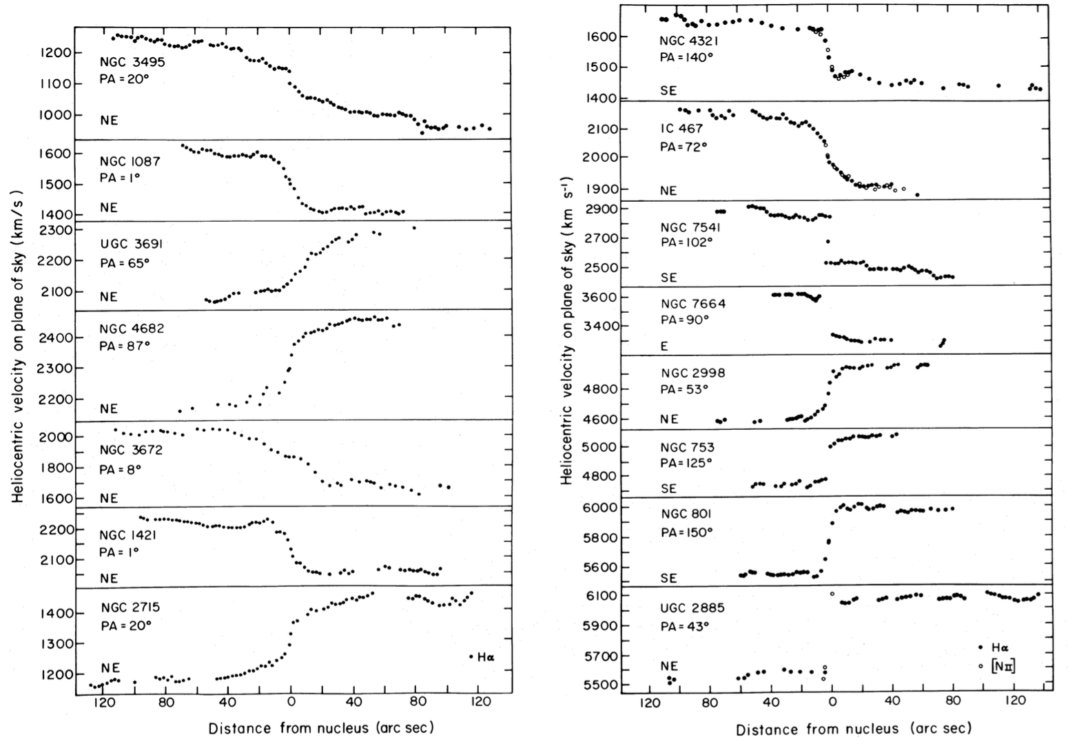
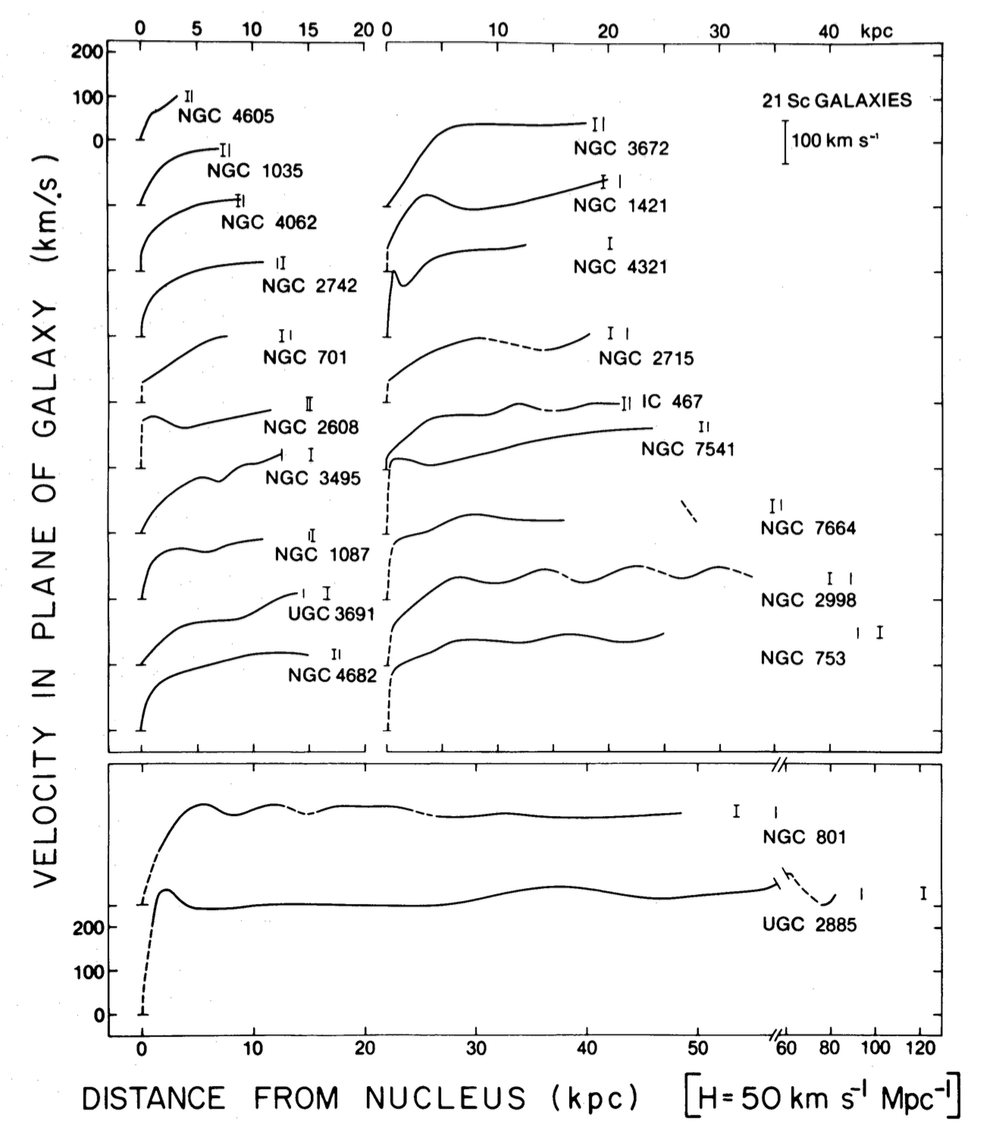
Traditionally, optical measurements are made with a long-slit spectrograph, which produces a one-dimensional trace. For reasons that will become clear below, this one-dimensional locus is best placed along the major axis (\(y=0\)) and these observations therefore produce \(V(x,0)\) in the notation above. A typical example are the velocity fields observed by Rubin et al. (1980):

(Credit: Rubin et al. 1980)

Integral-field observations now also routinely provide the full \(V(x,y)\) for optical emission lines (e.g., CALIFA: Sánchez et al. 2012; MaNGA: Bundy et al. 2015; SAMI: Croom et al. 2012).

CO and radio 21cm observations typically provide the two-dimensional velocity field \(V(x,y)\). A canonical example are the velocity fields of 22 spiral galaxies observed as part of Albert Bosma’s famous doctoral dissertation:

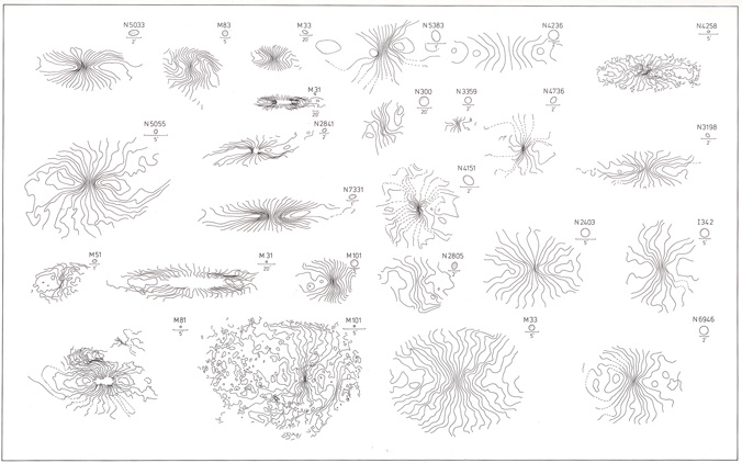
(Credit: Bosma 1978, available online here)

This figure shows contours of constant velocity and these velocity fields have all been oriented such that the major axis is horizontal for each galaxy. These velocity fields display all of the major types of features that one sees in two-dimensional velocity fields: (i) regions of vertical contours of constant velocities near the center, (ii) the spider-like shape of contours extending radially from the center, and (iii) closed contours along the major axis away from the center. We will discuss how all of these result from different types of galactic rotation and how we can essentially directly read off the rotation curve of these galaxies from these diagrams.

Two-dimensional velocity fields contain much more information than one-dimensional slices at \(y=0\) through them. In particular, they allow us to see deviations from circular rotation and from simple galactic geometry (for example, if the kinematic and photometric major axes do not coincide). Two-dimensional velocity fields are therefore essential to determining the best possible representation of a galaxy’s rotation curve, which we can define as follows: the velocity a test particle would have if it was on a circular orbit in an axially-symmetrized version of a galaxy’s mass distribution. By “axially-symmetrized” here we mean the galaxy’s mass distribution at radius \(R\) averaged around the axis perpendicular to the disk (this averages over, e.g., spiral structure’s deviations). We will discuss how we can determine a galaxy’s rotation curve from observations of its velocity field in Section 9.2.1 below.

Velocity fields remain one of the basic tools to learn about galactic structure, so before continuing with a detailed discussion of what they teach us about galactic rotation, we will look at a few more examples. The following is a map of the HI emission, optical emission, HI mean velocity field, and HI velocity dispersion for the galaxy NGC 3198 from the THINGS survey (Walter et al. 2008):

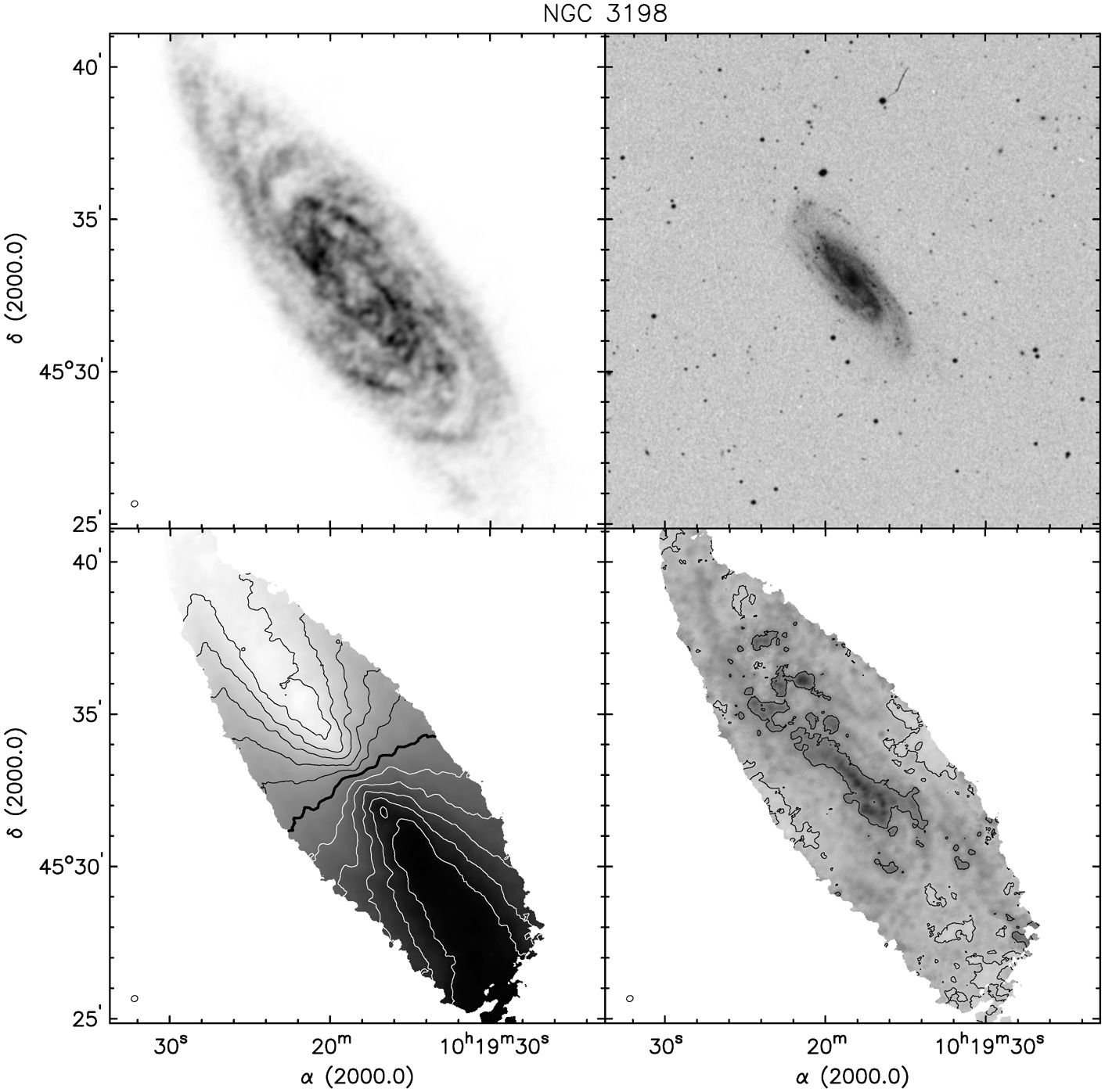
(Credit: Walter et al. 2008)

NGC 3198 is a galaxy famous for its rotation curve. After reading the next section, you should be able to immediately pinpoint why from the lower-left image. The observations extend out to about 40 kpc from the center and darker grayscale indicates receding velocities.

As a final example, through the use of adaptive-optics guided spectrographs we can now observe velocity fields of lines such as H\(\alpha\) for redshifts of one to three, allowing us to study galactic rotation and structure at earlier times in the Universe. For example, see the following figure with velocity fields for a selection of galaxies in the SINS H\(\alpha\) sample at redshifts in the range of one to three (Förster Schreiber et al. 2009):

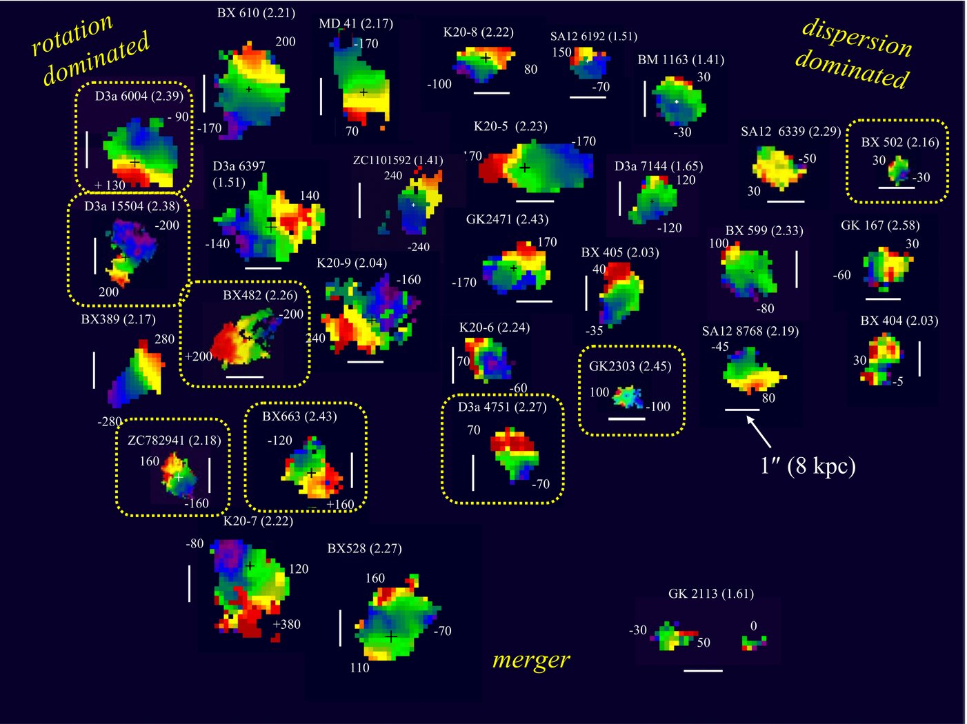
(Credit: Förster Schreiber et al. 2009)

With such H\(\alpha\) velocity fields being measured for more and more high-redshift galaxies, and with similar observations now starting for CO using the Northern Extended Millimeter Array (NOEMA; e.g., Uebler et al. 2018) and the Atacama Large Millimeter/submillimeter Array (ALMA), and with the coming resurgence of HI velocity fields from the Square Kilometer Array (SKA) and its precursors, the interpretation of velocity fields therefore remains as important as ever.

9.1.2. Velocity fields of axisymmetric disk galaxies

\label{sec-galrot-vfields}

To model galactic velocity fields, we consider a disk in circular rotation with rotation curve \(v_c(R)\), observed from our location (we will assume that the systemic velocity with respect to us is zero, because it simply adds a constant to all observed velocities). A location at radius \(R\) in the galaxy will have a velocity \(\vec{v} = -v_c(R)\,(\hat{\vec{R}}\times\hat{\vec{n}})\), where \(\hat{\vec{R}}\) is the unit vector that points to the location from the galaxy’s center and \(\hat{\vec{n}}\) is a unit vector normal to the disk plane. The observed line-of-sight velocity \(V\) is then the dot product of the velocity \(\vec{v}\) and the direction of the line-of-sight, \(\hat{\vec{r}}\), pointing from us to the galaxy:

\begin{align} V & = \hat{\vec{r}}\cdot\vec{v}\nonumber\\ & = v_c(R)\,\hat{\vec{R}}\,\cdot\left(\hat{\vec{r}}\times\hat{\vec{n}}\right)\nonumber\\ & = v_c(R)\,\hat{\vec{R}}\,\cdot\hat{\vec{k}}\,\sin i\label{eq-vlos-in-vfield}\,, \end{align}

where we have used that \(\vec{a}\cdot(\vec{b}\times\vec{c}) = -\vec{b}\cdot(\vec{a}\times\vec{c})\); \(i\) is the galaxy’s inclination (defined such that an an edge-on galaxy has an inclination of \(i=90^\circ\)) and \(\hat{k} = (\hat{\vec{r}}\times\hat{\vec{n}})/\sin i\) is the unit vector perpendicular to both \(\hat{\vec{r}}\) and \(\hat{\vec{n}}\).

Now we introduce a pair of two-dimensional coordinate systems. The first cartesian system \((x,y)\) is a system on the plane of the sky: we define the center such that the center of the galaxy is at \((x,y) = (0,0)\) and we orient the galaxy such that the major axis lies at \(y=0\). We will denote polar coordinates in this system as \((r,\phi)\). Then the projection of \(\hat{\vec{k}}\) points along \((1,0)\). The second coordinate system is in the plane of the galaxy and we will typically only consider polar coordinates \((R,\theta)\) for this system, but denote the cartesian coordinates as \((x',y')\) when we need them. The vector \(\hat{\vec{k}}\) lies in this plane and has (cartesian) components \((1,0)\); \(\hat{\vec{R}}\) also falls in this plane and has cartesian components \((\cos\theta,\sin\theta)\). Then Equation \(\eqref{eq-vlos-in-vfield}\) becomes

\begin{equation}\label{eq-twovfield-axi} V(x,y) = v_c(R)\,\cos\theta\,\sin i\,. \end{equation}

When we need to include a systemic velocity of the entire galaxy with respect to the observer, this simply adds a constant \(V_0\) to the left-hand side.

From the definition of the coordinate systems, we can derive a few useful relations between coordinates in the sky plane and those in the galaxy plane. We have that

\begin{align} x' & = x\,\\ y' & = \frac{y}{\cos i}\,, \end{align}

and

\begin{equation} \tan \theta = \frac{\tan \phi}{\cos i}\,. \end{equation}

Equation \(\eqref{eq-twovfield-axi}\) immediately makes it clear why when one is limited to observing a one-dimensional slice of the two-dimensional velocity field using long-slit spectroscopy, it is advantageous to observe along the major axis: \(\theta = 0\) or \(180^\circ\) there and we therefore have \(V(x,0) = \mathrm{sign(x)}\,v_c(R)\,\sin i\), the maximum observed velocity of any \(\theta\). Thus, the velocity along the major axis is simply the rotation velocity \(v_c(R)\) multiplied by the sine of the inclination. This produces the (reversed) S-shape behavior in the Rubin et al. (1980) curves above. But the mapping \(v_c(R) = V(x,0)/\sin i\) assumes that non-circular motions are unimportant.

To gain a better understanding of the observed velocity fields, we now look at a few simple examples.

9.1.3. Solid-body rotation

As discussed in Chapter 3.4.2, a homogeneous density distribution produces solid-body rotation with \(\Omega = v_c(R) / R = \mathrm{constant}\). If we plug this into Equation \(\eqref{eq-twovfield-axi}\) we get

\begin{equation} V(x,y) = \Omega\,R\,\cos\theta\,\sin i\,. \end{equation}

Because, \(x = x' = R\cos\theta\), this becomes simply

\begin{equation} V(x,y) = \Omega\,x\,\sin i\,. \end{equation}

The velocity therefore does not depend on \(y\) and contours of constant velocity will run parallel to the \(y\) axis. When we see vertical contours of constant velocity near the center of a two-dimensional velocity field, this is indicative of solid-body rotation. This is often observed in the velocity fields of external galaxies, for example in the examples from Bosma (1978) above.

9.1.4. A flat rotation curve

When we have a flat rotation curve, \(v_c(R) = v_c = \mathrm{constant}\), Equation \(\eqref{eq-twovfield-axi}\) becomes

\begin{align} V(x,y) & = v_c\,\cos\theta\,\sin i\nonumber\\ & = v_c\,\frac{x}{R}\,\sin i\nonumber\\ & = v_c\,\frac{\sin i\,\cos i}{\sqrt{\cos^2 i+\tan^2 \phi}}\,. \end{align}

Because the observed velocity only depends on \(\tan \phi\), it only depends on \(y/x\) and the contours of equal velocity are straight lines through the center. Thus, when we see regions of the two-dimensional velocity field of galaxies where the contours are straight lines pointing away from the center, this indicates that the rotation curve is flat in those regions

9.1.5. A peaked rotation curve

Finally, we consider what happens when the rotation curve of a galaxy rises to a maximum value and then declines. We write Equation \(\eqref{eq-twovfield-axi}\) as

\begin{equation} V(x,y) = v_c(R)\,\sin i\,\frac{x}{R}\,. \end{equation}

Along the \(y=0\), positive \(x\) locus, \(V(x,0) = v_c(R)\,\sin i\). When there are two different \(R_1\) and \(R_2\) at which a certain value of \(v_c\) is reached—one at a radius before the peak of the rotation curve, one after—this means that the value \(v_c\,\sin i\) is reached at two values along the \(x\) axis: at \(R_1\) and at \(R_2\). Similarly, along the same contour at fixed \(y\neq 0\), the same value \(V(x,y) = v_c(R_1)\,\sin i\) will be reached at two different \(x\), because if \(V(x_1,y)\) lies along the contours, then so does \(V(x_1\,R'_2/R'_1,y)\) where \(V(x_1\,R'_2/R'_1,y) = v_c(R'_1)\,\sin i\,x_1/R'_1\) and \(v_c(R'_1) = v_c(R'_2)\). Because \(x/R \leq 1\), if we follow a constant \(V\) contour starting at \(y=0\) upwards, it has to curve towards the \(x\) value at which the rotation curve peaks, because \(v_c(R)\) needs to increase to balance the decrease in \(x/R\) and maintain a constant \(V\). The contour keeps growing towards larger \(y\) until the required \(v_c(R)\) is the maximum value of the circular velocity. Then the contour turns down to decreasing \(y\) again until reaching the second value along \(y=0\) where the velocity is \(V\). The same happens when continuing down to negative \(y\) and all contours corresponding to \(V(x,0) = v_c(R)\,\sin i\) for \(v_c(R)\) that exist before and after the radius of maximum \(v_c\) therefore close.

Thus, if we see a closed contour in the two-dimensional velocity field \(V(x,y)\) of a galaxy, this means that the rotation curve reaches a maximum. Because for an isolated galaxy we assume that \(v_c(0) = v_c(\infty) = 0\), all contours should eventually close. But if the rotation curve does not decline within the observed area, then we may not see contours close within the observed area. And a single galaxy is of course not the only thing in the Universe, so practically a contour will not close if the circular velocity curve remains high into the surrounding environment.

In the velocity fields of Bosma (1978) and in that of NGC 3198 we see that the contours of the velocity field do not close for many of the observed galaxies, even though they extend out to dozens of kpc. Disk galaxies have light distributions that are observed to be exponential (Chapter 8.1) and if we assign a constant mass-to-light ratio to these galaxies, then the mass distribution should be that of an exponential disk. We computed the rotation curve for the exponential disk in Chapter 8.3.3.2 and found that it peaks at \(R \approx 2.15\,R_d\). Because galaxies have scale lengths \(R_d\) of a few kpc typically, we would therefore expect their rotation curves to peak at \(R \approx 10\,\mathrm{kpc}\) if their mass-to-light ratios are constant. Thus, we should see that contours in the velocity field start to close around \(R \approx 10\,\mathrm{kpc}\), but this is not what is observed.

9.1.6. Comparing different models and the cored logarithmic potential

\label{sec-galrot-coredlogpot}

The following figure summarizes what we have learned from these three examples. We define a general function that computes and plots the two-dimensional velocity field in Equation \(\eqref{eq-twovfield-axi}\) for any potential in galpy:

from galpy.potential import vcirc
def plot_twod_vfield(pot,sini=0.5,
                     title=None,
                     xmin=-2.,xmax=2.,nxs=100,
                     ymin=-2.,ymax=2.,nys=100,**kwargs):
    Vfield= numpy.empty((nxs,nys))
    xs= numpy.linspace(xmin,xmax,nxs)
    ys= numpy.linspace(ymin,ymax,nys)
    cos2i= 1.-sini**2.
    for ii in range(nxs):
        for jj in range(nys):
            R= numpy.sqrt(xs[ii]**2.+ys[jj]**2./cos2i)
            Vfield[ii,jj]= vcirc(pot,R)*xs[ii]/R*sini
    dx= xs[1]-xs[0]
    dy= ys[1]-ys[0]
    out= galpy_plot.dens2d(Vfield.T,origin='lower',
                           xrange=[xmin-dx/2.,xmax+dx/2.],
                           yrange=[ymin-dy/2.,ymax+dy/2.],
                           xlabel=r'$x$',ylabel=r'$y$',
                          **kwargs)
    if not title is None:
        annotate(title,(0.5,1.075),xycoords='axes fraction',
                 horizontalalignment='center',
                 verticalalignment='top',size=17.)
    return None

Then we apply this function to plot the rotation curve for the case of solid-body rotation, a flat rotation curve, and a rotation curve that peaks. For the latter, we use galpy’s Milky-Way potential model, MWPotential2014, which peaks at \(R\approx0.5\). We use \(\sin i = 0.5\).

from galpy import potential
figsize(14,5)
subplot(1,3,1)
# size R of homogeneous >> considered region
hp= potential.HomogeneousSpherePotential(normalize=1.,R=10.)
plot_twod_vfield(hp,contours=True,cmap='bwr',gcf=True,
                 title=r'$v_c(R) = \Omega\,R$')
subplot(1,3,2)
lp= potential.LogarithmicHaloPotential(normalize=1.)
plot_twod_vfield(lp,contours=True,cmap='bwr',gcf=True,
                title=r'$v_c(R) = v_c = \mathrm{constant}$')
subplot(1,3,3)
plot_twod_vfield(potential.MWPotential2014,contours=True,cmap='bwr',
                 levels=numpy.linspace(-.5,.5,21),gcf=True,
                title=r'$\mathrm{peaked}\, v_c(R)$')
tight_layout()

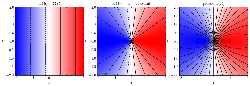
These velocity fields agree with our theoretical work above: the solid-body rotation curve gives rise to vertical constant-velocity contours, the flat rotation curve gives radial contours, and the peak in the rotation curve in the right panel causes closed contours along the major axis. The rotation curve on the right drops off very slowly beyond the peak, which is why there are only two closed contours in this figure.

To demonstrate the latter point, we compare the velocity field of a Kuzmin disk and that of a razor-thin exponential disk with the same mass and with the same peak radius. We compared the rotation curves for these two models in Chapter 8.3.3.2, where we found that the exponential disk peaks at a higher value and that it is therefore more peaked. The two-dimensional velocity fields display this clearly:

figsize(10,5)
subplot(1,2,1)
kzp= potential.KuzminDiskPotential(amp=10.,a=2.15/numpy.sqrt(2.))
rp= potential.RazorThinExponentialDiskPotential(amp=10./(2.*numpy.pi),hr=1.)
levels= numpy.linspace(-1.,1.,16)
plot_twod_vfield(kzp,contours=True,cmap='bwr',gcf=True,
                xmin=-7.,xmax=7.,ymin=-7.,ymax=7.,levels=levels,
                title=r'$\mathrm{Kuzmin}$')
subplot(1,2,2)
plot_twod_vfield(rp,contours=True,cmap='bwr',gcf=True,
                xmin=-7.,xmax=7.,ymin=-7.,ymax=7.,levels=levels,
                title=r'$\mathrm{Exponential}$')

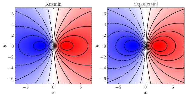
The more peaked nature of the exponential-disk’s rotation curve leads to tighter closed contours than in the case of the Kuzmin disk (the contours in the above figure are at the same level in both panels). Thus, from the tightness of the closed contours in a two-dimensional velocity field (if there are any), we can directly read off how peaked the rotation curve is.

However, as we will discuss in more detail below, two-dimensional velocity fields typically do not have closed contours, indicating that their rotation curves remain flat out to the observed radius (NGC 3198 above is a good example of this). In that case, we should see a velocity pattern that corresponds to a rising rotation curve that flattens at a certain radius. A simple model with this behavior is a cored logarithmic potential: \(\Phi(R) = v^2_0 \ln[R_c^2+R^2]/2\), which has \(v_c(R) = v_0\,R/\sqrt{R^2+R^2_c}\). At \(R \ll R_c\) , this corresponds to solid-body rotation and at \(R \gg R_c\) the rotation curve is flat; this model is therefore a good representation of a rising-to-flat rotation curve. The velocity field of this model with \(R_c = 0.25\) is

lp= potential.LogarithmicHaloPotential(normalize=1.,core=0.25)
plot_twod_vfield(lp,contours=True,cmap='bwr',gcf=True,
                 levels=numpy.linspace(-0.5,0.5,13),
                 title=r'$\mathrm{Rising\ to\ flat}$')

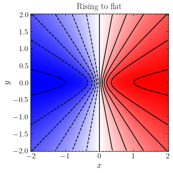
The velocity field goes from the vertical-contour behavior of solid-body rotation near \(x=0\) to the radial behavior of a flat rotation curve at larger \(|x|\). This pattern is very close to the pattern observed in many of the two-dimensional velocity field pictured at the beginning of this chapter, e.g., that of NGC 3198.

9.2. Rotation curves of external galaxies

\label{sec-galrot-velfield-extgals}

In the previous section, we described two-dimensional velocity fields of external galaxies and how features in these fields relate to the underlying rotation of the galaxy. Now that we understand the basic structure of two-dimensional velocity fields, we can focus our attention on how we can determine the one-dimensional rotation curve from these fields and how we can use it to determine the mass distribution of galaxies and find convincing evidence of the existence of dark matter.

9.2.1. From velocity fields to rotation curves

\label{sec-galrot-velfield-to-rotcurve}

There are various methods for extracting the one-dimensional rotation curve \(v_c(R)\) of a galaxy from a map of its two-dimensional velocity field \(V(x,y)\). The simplest of these uses the fact that \(V(x,0) = \mathrm{sign(x)}\,v_c(R)\,\sin i\) and therefore

\begin{equation}\label{eq-vc-from-vxy-simple} v_c(R) = \frac{V(x,0)}{\sin i\,\mathrm{sign(x)}}\,. \end{equation}

If we have actually determined the two-dimensional field \(V(x,y)\), then this method throws out much information, but as we have discussed, many observations—especially using optical spectroscopy—only determine \(V(x,0)\), not the full two-dimensional field \(V(x,y)\). Using Equation \(\eqref{eq-vc-from-vxy-simple}\) is then the only option to extract the rotation curve. The galaxy’s inclination needs to be known from photometric observations, because otherwise it is degenerate with \(v_c(R)\). One simple way to estimate the inclination for a disk galaxy is to assume that its face-on shape is circular, such that the elliptical shape of observed isophotes is solely due to the inclination’s projection effect.

When we have measured the full 2D \(V(x,y)\) field, we can use Equation \(\eqref{eq-twovfield-axi}\) and fit for the free parameters. This typically includes the center of the galaxy on the sky \((x_0,y_0)\) (which we have set to \((0,0)\) in the discussion so far), the angle \(\phi_0\) of the galaxy’s major axis at the receding-velocity side, typically measured counter-clockwise from the north (which we set to \(\phi_0 = 180^\circ\) above), the systemic velocity of the galaxy \(V_0\) (which we set to zero above), the inclination \(i\) if not fixed by photometric observations, and parameters describing \(v_c(R)\). A popular method for performing the fit is to perform it in a set of annuli around the center of the galaxy, where each annulus can in principle have its own value for all of the parameters that we mentioned. Because the annuli can be tilted with respect to each other when they have different \((i,\phi_0)\), this method is known as the tilted-ring model (e.g., Begeman 1989). To account for any deviations from circular rotation, these fits also often include a radial term \(v_r(R)\) to model radial motions in the plane.

Including all parameters, the observed velocity field is given by

\begin{equation} V(x,y) = V_0 + v_c(R)\,\cos\theta\,\sin i + v_r(R)\,\sin\theta\,\sin i\,, \end{equation}

where

\begin{align} \cos \theta& = \frac{-(x-x_0)\,\sin \phi_0+(y-y_0)\,\cos \phi_0}{R}\,,\\ \sin \theta& = \frac{-(x-x_0)\,\cos \phi_0-(y-y_0)\,\sin \phi_0}{R\,\cos i}\,. \end{align}

In practice, parameters such as \((x_0,y_0)\) are typically fixed to be (i) the same for each tilted ring and (ii) determined by the photometric center.

9.2.2. Observed rotation curves

\label{sec-galrot-obsrotcurves}

Now that we know how to extract rotation curves from observed velocity fields, let us look at some classical results on rotation curves. We start by looking at the rotation curves derived from the one-dimensional velocity fields from Rubin et al. (1980) that we displayed at the start of this chapter:

(Credit: Rubin et al. 1980 )

The vertical line segments in this figure are the so-called “optical radius” \(R_{25}\), which is defined as the radius corresponding to the isophote where the surface brightness is \(25\,\mathrm{mag\,arcsec}^{-2}\). This is a convenient definition of the radius of a galaxy’s light, because galaxies emit little light outside of this radius. Most of the rotation curves do not reach the optical radius, but they typically get close. We would therefore expect to see the rotation curve turn over if these disk galaxies were pure exponential disks. However, the rotation curves remain mostly flat at the largest observed radius.

Kent (1986) obtained photometry for these galaxies and asked the question: can these rotation curves be fit with constant mass-to-light ratios and are the mass-to-light ratios reasonable considering our knowledge of stellar population from which we expect mass-to-light ratios of a few (see also Kalnajs 1983). To answer this question, Kent (1986) measured the surface-brightness profile \(\mu(R)\) of these galaxies and decomposed them into a bulge \(\mu_b(R)\) and a disk \(\mu_d(R)\) component, each of which is allowed to have a different constant mass-to-light ratio, \((M/L)_b\) and \((M/L)_d\), respectively. The total surface density is then

\begin{align} \Sigma(R) & = \Sigma_b(R) + \Sigma_d(R)\nonumber\\ & = (M/L)_b\,\mu_b(R) + (M/L)_d\,\mu_d(R)\,. \end{align}

We can use the framework from the previous chapter to determine the circular velocity profile \(v_c(R)\) corresponding to this surface density profile.

For the bulge, we may assume that the underlying mass distribution is spherical. We then first need to deproject the observed surface-density profile, using the inversion equation (7.16) to obtain the luminosity density \(\nu_b(r)\)

\begin{equation} \nu_b(r) = -\frac{1}{\pi}\,\int_r^\infty\mathrm{d}R\,\frac{\mathrm{d} \mu(R)}{\mathrm{d} R}\,\frac{1}{\sqrt{R^2-r^2}}\,. \end{equation}

and then integrate this to obtain the enclosed luminosity profile \(L_b(<r)\)

\begin{equation} L_b(<r) = 4\pi\,\int_0^r\,\mathrm{d}s\,s^2\,\nu_b(s)\,. \end{equation}

The circular velocity from the bulge component is then simply given by

\begin{equation}\label{eq-vcb-kent} v_{c,b}^2(r) = \left(\frac{M}{L}\right)_b\,\frac{G\,L_b(<r)}{r}\,. \end{equation}

To obtain the contribution of the disk component \(v_{c,d}^2(r)\), we start with the expression for the circular velocity of a razor-thin disk as a function of the surface density from Equation (8.39). We can write this equation in a more convenient form for applying to an arbitrary \(\Sigma_d = (M/L)_d\,\,\mu_d(R)\) as

\begin{align} v_{c,d}^2(R) & =2\pi\,G\,R\,(M/L)_d\,\int_0^\infty\mathrm{d}k\,\,J_1(kR)\,k\,\int_0^\infty \mathrm{d} R' \,J_0(kR')\,R'\,\mu_d(R')\nonumber\\ & =2\pi\,G\,R\,(M/L)_d\,\int_0^\infty \mathrm{d} R'\,R'\,\mu_d(R')\,\int_0^\infty\mathrm{d}k\,\,J_1(kR)\,k\, \,J_0(kR')\nonumber\\ & =-2\pi\,G\,R\,(M/L)_d\,\int_0^\infty \mathrm{d} R'\,R'\,\mu_d(R')\,\frac{\mathrm{d}}{\mathrm{d}R}\left[\int_0^\infty\mathrm{d}k\,\,J_0(kR)\,\,J_0(kR')\right]\, \end{align}

The integral in square brackets is a simpler version of an integral that we encountered in Equation (8.42), which we can also write as

\begin{equation} \int_0^\infty\mathrm{d}k\,J_0(kR) \,J_0(kR') = \frac{2}{\pi}\begin{cases}\frac{1}{R}\,\,K\left(\left[\frac{R'}{R}\right]^2\right) & R' < R\\ \frac{1}{R'}\,\,K\left(\left[\frac{R}{R'}\right]^2\right) & R' < R\\\end{cases}\,, \end{equation}

where \(K(m)\) is the complete elliptic integral of the first kind. Therefore,

\begin{align} v_{c,d}^2(R) = 4\,G\,(M/L)_d\,&\Bigg\{ \int_0^R \mathrm{d} R'\,\mu_d(R')\frac{R'}{R}\,\frac{E(m)}{(1-m)}\nonumber\\ & \ + \int_R^\infty \mathrm{d} R'\,\mu_d(R')\,\left[K(m^{-1})-\frac{E(m^{-1})}{1-m^{-1}}\right]\Bigg\}\,,\label{eq-vcd-kent} \end{align}

where \(m=(R'/R)^2\). This integral—which has an integrable singularity at \(R = R'\), so some care needs to be taken in its numerical calculation—allows us to compute the rotation curve for any razor-thin disk \(\Sigma_d(R) = (M/L)_d\,\mu_d(R)\). For a given \(\mu_d(R)\), we can compute the function in the curly brackets once and then adjust the mass-to-light ratio \((M/L)_d\) to change \(v_{c,d}^2(R)\). We could have also derived this expression for the circular velocity by starting from the general expression for the gravitational potential of any axisymmetric, razor-thin disk in Equation (8.65).

By combining Equations \(\eqref{eq-vcb-kent}\) and \(\eqref{eq-vcd-kent}\), we can then compute the rotation curve corresponding to the observed bulge and disk surface brightness for different values of \((M/L)_b\) and \((M/L)_d\). We can then ask whether we can fit the entire rotation curve if we adjust the mass-to-light ratios such that they provide a good fit to the rotation curve in the inner region. These are known as maximum-disk fits, because we set the mass-to-light ratios to the largest possible value—any larger and the computed inner rotation curve would be larger than the observed one. Kent (1986) did this for many galaxies, here is the result for two of them that demonstrates the two different situations that occur:

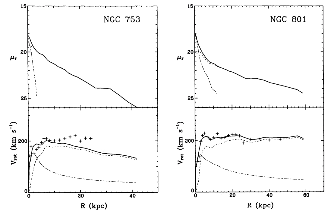
(Credit: Kent 1986; note that \(\mu(R)\) in this figure is the surface brightness expressed in logarithmic units \(\mathrm{mag\,arcsec}^{-2}\))

These figures display the observed surface-brightness profile \(\mu(R)\) and its decomposition into bulge \(\mu_b(R)\) and disk \(\mu_d(R)\) components in the top panel. The bottom panels show the observed rotation curve and the maximum-disk fits described above.

We see that in the case of NGC 801 the maximum-disk fit provides an excellent match to the entire observed rotation curve, even though the rotation curve extends to 50 kpc. Thus, there appears to be no need for additional matter. The NGC 801 fit has \((M/L)_b \approx 1.5\) and \((M/L)_d \approx 7\); the maximum-disk fit therefore requires a somewhat high mass-to-light ratio. But nevertheless, it is remarkable that NGC 801’s rotation curve and surface brightness can be fit without including any halo dark matter (at least in 1986, see below).

NGC 753, however, displays very different behavior. The maximum-disk fit successfully reproduces the inner (\(R \lesssim 10\,\mathrm{kpc}\)) rotation curve, but because the surface-brightness profile steeply declines at large radii, the maximum-disk rotation curve drops at \(R \gtrsim 10\,\mathrm{kpc}\). The observed rotation curve, however, remains approximately constant. The mass-to-light ratios for NGC 753’s maximum-disk fit are reasonable: \((M/L)_b \approx 3\) and \((M/L)_d \approx 1.2\). Therefore, it is clear that we need an additional component to explain NGC 753’s rotation curve. Equivalently, the mass-to-light ratio needs to increase with \(R\).

It is instructive to look through the other fits in the Kent (1986) paper. Most of the galaxies considered behave similar to NGC 801: the maximum-disk rotation curve can explain the entire observed rotation curve, except for perhaps the last few points. This demonstrates the difficulty in using optical rotation curves to constrain the mass-to-light ratio in the outer regions of galaxies: these curves typically do not extend far enough to unambiguously show the influence of dark matter.

We can repeat Kent (1986)’s analysis using more modern data. The SPARC (Spitzer Photometry and Accurate Rotation Curves) sample of Lelli et al. (2016) consists of 175 nearby galaxies with mid-infrared photometry photometry from the Spitzer space telescope (at \(3.6\,\mu\mathrm{m}\)) and precise rotation curves from 21cm and H\(\alpha\) observations.

To use this data here, we first implement a general function to download the data from Vizier, which we wil also use elsewhere:

# vizier.py: download catalogs from Vizier
import sys
import os, os.path
import shutil
import tempfile
from ftplib import FTP
import subprocess
_ERASESTR= "                                                                                "
def vizier(cat,filePath,ReadMePath,
           catalogname='catalog.dat',readmename='ReadMe'):
    """
    NAME:
       vizier
    PURPOSE:
       download a catalog and its associated ReadMe from Vizier
    INPUT:
       cat - name of the catalog (e.g., 'III/272' for RAVE, or J/A+A/... for journal-specific catalogs)
       filePath - path of the file where you want to store the catalog (note: you need to keep the name of the file the same as the catalogname to be able to read the file with astropy.io.ascii)
       ReadMePath - path of the file where you want to store the ReadMe file
       catalogname= (catalog.dat) name of the catalog on the Vizier server
       readmename= (ReadMe) name of the ReadMe file on the Vizier server
    OUTPUT:
       (nothing, just downloads)
    HISTORY:
       2016-09-12 - Written as part of gaia_tools - Bovy (UofT)
       2017-09-12 - Copied to galdyncourse (yes, same day!) - Bovy (UofT)
       2019-12-20 - Copied directly into notes to avoid additional dependency - Bovy (UofT)
    """
    _download_file_vizier(cat,filePath,catalogname=catalogname)
    _download_file_vizier(cat,ReadMePath,catalogname=readmename)
    catfilename= os.path.basename(catalogname)
    with open(ReadMePath,'r') as readmefile:
        fullreadme= ''.join(readmefile.readlines())
        if catfilename.endswith('.gz') and not catfilename in fullreadme:
            # Need to gunzip the catalog
            try:
                subprocess.check_call(['gunzip',filePath])
            except subprocess.CalledProcessError as e:
                print("Could not unzip catalog %s" % filePath)
                raise
    return None

def _download_file_vizier(cat,filePath,catalogname='catalog.dat'):
    sys.stdout.write('\r'+"Downloading file %s from Vizier ...\r" \
                         % (os.path.basename(filePath)))
    sys.stdout.flush()
    try:
        # make all intermediate directories
        os.makedirs(os.path.dirname(filePath))
    except OSError: pass
    # Safe way of downloading
    downloading= True
    interrupted= False
    file, tmp_savefilename= tempfile.mkstemp()
    os.close(file) #Easier this way
    ntries= 1
    while downloading:
        try:
            ftp= FTP('cdsarc.u-strasbg.fr')
            ftp.login()
            ftp.cwd(os.path.join('pub','cats',cat))
            with open(tmp_savefilename,'wb') as savefile:
                ftp.retrbinary('RETR %s' % catalogname,savefile.write)
            shutil.move(tmp_savefilename,filePath)
            downloading= False
            if interrupted:
                raise KeyboardInterrupt
        except:
            raise
            if not downloading: #Assume KeyboardInterrupt
                raise
            elif ntries > _MAX_NTRIES:
                raise IOError('File %s does not appear to exist on the server ...' % (os.path.basename(filePath)))
        finally:
            if os.path.exists(tmp_savefilename):
                os.remove(tmp_savefilename)
        ntries+= 1
    sys.stdout.write('\r'+_ERASESTR+'\r')
    sys.stdout.flush()
    return None

We then write a function to download the SPARC data and store it in a cache directory $HOME/.galaxiesbook/cache/vizier (this directory will be automatically created on your system):

import os, os.path
from astropy.io import ascii
_CACHE_BASEDIR= os.path.join(os.getenv('HOME'),'.galaxiesbook','cache')
_CACHE_VIZIER_DIR= os.path.join(_CACHE_BASEDIR,'vizier')
_LELLI_VIZIER_NAME= 'J/AJ/152/157'
def download_sparc(verbose=False):
    """
    NAME:
       download_sparc
    PURPOSE:
       download and read the Lelli et al. (2016) catalog of
       rotation curves and photometry for galaxies
       in the SPARC sample
    INPUT:
       verbose= (False) if True, be verbose
    OUTPUT:
       pandas dataframe
    HISTORY:
       2021-01-05 - Written - Bovy (UofT)
    """
    # Generate file path and name
    tPath= os.path.join(_CACHE_VIZIER_DIR,'cats',
                        *_LELLI_VIZIER_NAME.split('/'))
    filePath= os.path.join(tPath,'table2.dat')
    readmePath= os.path.join(tPath,'ReadMe')
    # download the file
    if not os.path.exists(filePath):
        vizier(_LELLI_VIZIER_NAME,filePath,readmePath,
               catalogname='table2.dat',readmename='ReadMe')
    # Read with astropy
    table= ascii.read(filePath,readme=readmePath,format='cds')
    return table.to_pandas()

and a function to read the data for a single galaxy

def read_sparc_data(galaxy):
    """Return the data for a given galaxy"""
    raw= download_sparc()
    return raw[raw['Name'] == galaxy]

Then we write some functions to deal with the surface brightness profile. We will only deal with galaxies that only have a small bulge component and we will ignore this bulge component, instead assuming that the entire surface brighness is contributed by the disk (that is, in the notation above, we assume that \(\mu(R) = \mu_d(R)\) and \(v_c(R) = v_{c,d}(R)\)). This assumption only affects the rotation curve within the inner few kpc. The following function plots the surface brightness as a function of radius for a given galaxy:

def plot_sparc_lumprofile(galaxy):
    data= read_sparc_data(galaxy)
    semilogy(data['Rad'],data['SBdisk'],
             marker='o',ls='none',color='k',zorder=1)
    xlim(0.,1.1*numpy.amax(data['Rad']))
    ylim(0.5**numpy.amax(data['SBdisk']),
         2*numpy.amax(data['SBdisk']))
    xlabel(r'$R\,(\mathrm{kpc})$')
    ylabel(r'$\mu\,(L_\odot\,\mathrm{pc}^{-2})$')
    galpy_plot.text(r'$\mathrm{{{}}}$'.format(
        '\ '.join([s  if (len(s) < 2 or s[0] != '0')
                      else s[1:]
                      for s in re.split(r'(\d+)',galaxy)])),
                    size=18.,top_right=True)
    return [0.,1.1*numpy.amax(data['Rad'])]

Next we create a class to build a simple model for the surface brightness profile \(\mu(R)\): a cubic spline through the observed data points. We also implement a function to plot the model luminosity profile:

from scipy import interpolate
class model_lumprofile():
    # By 'lumprofile' we mean surface-brightness profile here
    def __init__(self,galaxy):
        data= read_sparc_data(galaxy)
        data= data[data['SBdisk'] > 0]
        self._Rmin= numpy.amin(data['Rad'])
        self._Rmax= numpy.amax(data['Rad'])
        self._lum_at_Rmin= numpy.array(data['SBdisk'])[numpy.argmin(data['Rad'])]
        self._ip= interpolate.InterpolatedUnivariateSpline(\
                    data['Rad'],numpy.log(data['SBdisk']),k=3)
    def __call__(self,R):
        R= numpy.atleast_1d(R)
        # We assume that mu(R) is zero beyond the last data point
        # and constant within the innermost data point
        out= numpy.zeros(R.shape)
        if isinstance(R,u.Quantity):
            R= R.to_value(u.kpc)
        oindx= (R >= self._Rmin)*(R <= self._Rmax)
        out[oindx]= numpy.exp(self._ip(R[oindx]))
        oindx= R < self._Rmin
        out[oindx]= self._lum_at_Rmin
        return out*u.Lsun/u.pc**2
def plot_model_lumprofile(RRange,lumprofile):
    Rs= numpy.linspace(RRange[0],RRange[1],101)
    plot(Rs,lumprofile(Rs),lw=2.,zorder=10)
    return None

Next, we define a function to plot the observed rotation curve:

def plot_sparc_rotcurve(galaxy):
    data= read_sparc_data(galaxy)
    errorbar(data['Rad'],data['Vobs'],yerr=data['e_Vobs'],
             marker='o',ls='none',color='k',zorder=1)
    xlim(0.,1.1*numpy.amax(data['Rad']))
    ylim(0.,1.3*numpy.amax(data['Vobs']))
    xlabel(r'$R\,(\mathrm{kpc})$')
    ylabel(r'$v_c\,(\mathrm{km\,s}^{-1})$')
    return [0.,1.1*numpy.amax(data['Rad'])]

With the model for the observed surface brightness profile, we can now use Equation \eqref{eq-vcd-kent} to turn this profile into a predicted rotation curve using a mass-to-light ratio \(M/L\). We can do this using galpy’s AnyAxisymmetricRazorThinDiskPotential, which implements Equation \eqref{eq-vcd-kent} (in fact, a more general version that includes the full potential and all its derivatives):

from galpy.potential import AnyAxisymmetricRazorThinDiskPotential
def model_diskpot(MoverL,lumprofile):
    return AnyAxisymmetricRazorThinDiskPotential(\
                lambda R: MoverL*lumprofile((R/u.kpc).to_value(u.dimensionless_unscaled)),
                                                 ro=8.,vo=220.)
def plot_model_diskrotcurve(RRange,diskpot):
    Rs= numpy.linspace(RRange[0],RRange[1],101)
    plot(Rs,[diskpot.vcirc(R*u.kpc).to_value(u.km/u.s) for R in Rs],lw=2.,zorder=10)
    return None

Finally, we put everything together to plot the observed surface brightness profile and rotation curve for a galaxy and the model resulting from applying Equation \eqref{eq-vcd-kent} for an assumed mass-to-light ratio:

from matplotlib import gridspec
from matplotlib.ticker import FuncFormatter
def plot_sparc(galaxy,gs):
    subplot(gs(0))
    plot_sparc_lumprofile(galaxy)
    gca().yaxis.set_major_formatter(FuncFormatter(
                lambda y,pos: (r'${{:.{:1d}f}}$'.format(int(\
                    numpy.maximum(-numpy.log10(y),0)))).format(y)))
    gca().tick_params(labelbottom=False)
    subplot(gs(1))
    plot_sparc_rotcurve(galaxy)
    return None
def plot_sparc_model(MoverL,galaxy,gs):
    lumprofile= model_lumprofile(galaxy)
    subplot(gs(0))
    data= read_sparc_data(galaxy)
    model_RRange= [numpy.amin(data['Rad']),numpy.amax(data['Rad'])]
    plot_model_lumprofile(model_RRange,lumprofile)
    subplot(gs(1))
    diskpot= model_diskpot(MoverL,lumprofile)
    plot_model_diskrotcurve(model_RRange,diskpot)
    return None

Let’s now look at some of the galaxies that Kent (1986) studied as well. NGC 753 is not part of the SPARC sample, but NGC 801 is, so we can revisit it. We’ll also look at NGC 2998. We choose a mass-to-light ratio that maximizes the disk contribution, by setting it as high as we can without predicting a circular velocity that is too much above the observed rotation curve in the inner galaxy (we allow the prediction to be a bit high in the inner ten kpc, because we are ignoring the bulge, which would predict a smaller rotation velocity for the same surface brightness).

figsize(10,7)
gs= gridspec.GridSpec(ncols=2,nrows=2,hspace=0.,
                     height_ratios=[2,1])
plot_sparc('NGC2998',lambda i: gs[i,0])
plot_sparc_model(0.9*u.Msun/u.Lsun,'NGC2998',lambda i: gs[i,0])
plot_sparc('NGC0801',lambda i: gs[i,1])
plot_sparc_model(0.6*u.Msun/u.Lsun,'NGC0801',lambda i: gs[i,1])
tight_layout();

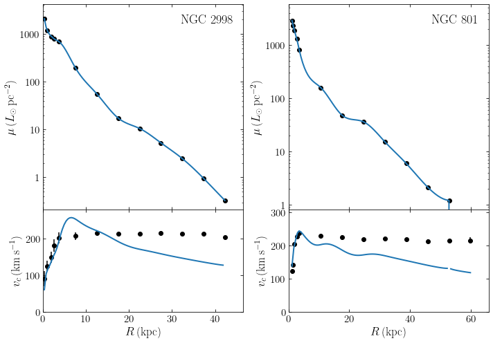
We see that in both cases, the predicted rotation curve for the maximum-disk fit peaks at 5 to 10 kpc from the center and then decays to a value that is just over half of the observed value at the largest radius. We also see that the predicted disk rotation curve for NGC 801 decays rather than staying flat in the Kent (1986) analysis. This is because the more accurate and precise Spitzer photometry displays a steeper decline than the photometry used by Kent (1986). The mass-to-light ratios of \(M/L \approx 1\) are reasonable for the mid-infrared photometric bandpass used by SPARC.

Thus, we see that the combination of the modern photometric and rotation curve data for the disk galaxies observed by Rubin et al. (1980) clearly indicate that the mass-to-light ratio increases significantly with radius (by a factor of approximately four for the galaxies that we looked at).

Radio observations of the 21cm line of neutral hydrogen allow the velocity field to be mapped at larger distances than the optical rotation curves that we have discussed so far. At the start of this chapter, we showed the velocity maps from Bosma (1978) (which surely must be one of the most highly-cited PhD theses in astronomy). Many of these extend to beyond the optical radius of the galaxy, typically to between the optical radius and twice that radius. Therefore, we expect to approach the Keplerian drop-off in the rotation curves in the outer observed regions and we should see clear closed contours in the two-dimensional velocity maps \(V(x,y)\). However, looking at the velocity maps, we see that closed contours are rare and that most of the galaxies in Bosma’s sample have the “spider” shape indicative of flat rotation curves.

Bosma used a tilted-ring model to extract the one-dimensional rotation curves from the two-dimensional velocity fields. The figure below displays the resulting rotation curves, arranged by Hubble type (the “Galaxy” rotation curve is that of the Milky Way, which we will come back to below):

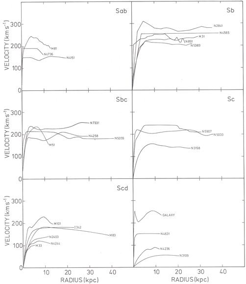
(Credit: Bosma 1978)

The rotation curves of the majority of these galaxies remain flat to the furthest observed point, typically well beyond the optical radius of the galaxy. Without good optical photometry for these galaxies, Bosma (1978) could not do an analysis of the type performed by Kent (1986) for the Rubin et al. (1980) sample above. Instead, Bosma (1978) attempted an inversion of the observed \(v_c(R)\) to \(\Sigma(R)\) and \(M(<R)\) assuming either (i) that the mass was distributed as a razor-thin disk with a to-be-determined surface density \(\Sigma(R)\) or (ii) that the mass was made up of spheroidal and simple disk components with to-be-determined parameters. The first of these methods is problematic, because determining a razor-thin disk’s \(\Sigma(R')\) at a radius \(R'\) requires knowledge of \(v_c(R)\) at large \(R\), but the rotation curves are observed to be flat at all \(R\), so extrapolating to the necessary decline at large \(R\) is difficult. However, no matter what method is used to determine \(M(<R)\) from the observed rotation curve, mass profiles similar to Bosma (1978)’s would result. The following figure displays the derived mass profiles:

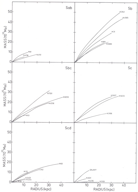
(Credit: Bosma 1978)

As expected from our discussion in Chapter 3.3, a flat rotation curve implies \(M(<R) \propto R\) and this is indeed what can be seen in the figure above. These galaxies have large masses enclosed within the radius of the last point where \(v_c(R)\) was measured and the mass should be expected to keep rising, because the increase barely flattens at large radius. These masses are larger by a factor of at least a few than the mass observed within the optical radius (which can be read off from \(M(<R)\) at the optical radius and requires no mass-to-light assumptions). These radio observations therefore leave no doubt about the presence of a large amount of dark matter in these galaxies.

Finally, let’s look at one of the best poster childs for flat rotation curves: NGC 3198. We displayed the two-dimensional velocity field \(V(x,y)\) from the THINGS survey at the start of this chapter. That velocity field beautifully shows the vertical contours near the center (perpendicular to the major axis) indicative of solid-body rotation and the spider-like contours outside of the center indicative of a flat rotation curve. A tilted-ring analysis leads to the following rotation curve for NGC 3198:

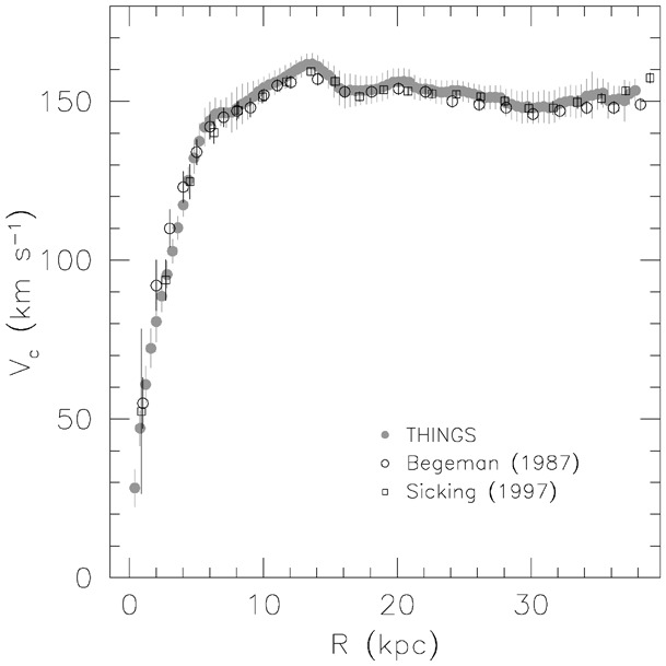
(Credit: de Blok et al. 2008)

The scale length of the light profile of NGC 3198 is \(\approx 2.7\,\mathrm{kpc}\) (van Albada et al. 1985) and the optical radius is about 10 kpc. This rotation curve therefore extends out to about 11 disk scale lengths or four times the optical radius. Looking at the rotation curve of an exponential disk in Chapter 8.3.3.2, we see that at 11 disk scale lengths the rotation velocity should be less than half of the maximum rotation velocity and we should see a strong decline in the rotation velocity that is essentially Keplerian. That the actual rotation curve is flat means that NGC 3198 must have a large amount of matter beyond the optical radius: approximately four times as much (van Albada et al. 1985). This is confirmed by repeating our Kent (1986)-style analysis using the SPARC data. For a mid-infrared mass-to-light ratio of \(M/L = 0.8\), we find

figsize(5,7)
gs= gridspec.GridSpec(ncols=1,nrows=2,hspace=0.,height_ratios=[2,1])
plot_sparc('NGC3198',lambda i: gs[i,0])
plot_sparc_model(0.8*u.Msun/u.Lsun,'NGC3198',lambda i: gs[i,0])

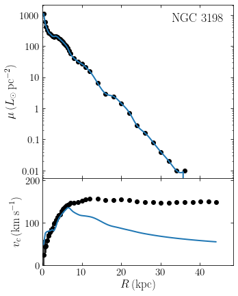
Because the surface brightness profile is so close to exponential with a scale length of \(\approx 2.7\) kpc, we see that the rotation curve peaks at \(R \approx 6\) kpc as expected for an exponential disk (which peaks at \(R \approx 2.15\,R_d\), see Equation 8.56). The rotation curve predicted from the stellar luminosity alone then steadily declines and the mass-to-light ratio must increase with radius to counter-act this predicted decline for a constant mass-to-light ratio.

Thus, we see that the evidence from HI rotation curves of external galaxies is clear: galaxies must be surrounded by an extended distribution of non-luminous, dark matter that causes the total mass-to-light ratio to increase with radius.

9.3. The kinematics of the Milky Way’s interstellar medium

9.3.1. The longitude-velocity diagram

\label{sec-galrot-lv}

In the Milky Way, we can also observe the kinematics of tracers such as HI and CO to study galactic rotation. A complication, however, is that the observer’s (i.e., our own) position is itself participating in the rotation of the disk and the observed velocities of the gas therefore reflect both intrinsic galactic rotation as well as the motion of the Sun and Earth. This greatly complicates measuring the rotation curve of the Milky Way from the kinematics of the interstellar medium (or from the kinematics of any disk tracer really). Despite this complication, the kinematics of the interstellar medium contains a wealth of information about the rotation of the Milky Way and perturbations to circular rotation from the influence of, e.g., the bar and spiral structure. In this section we will only consider motions in the mid-plane of the Milky Way and ignore the motion perpendicular to the mid-plane, because we may assume that gas orbits in the mid-plane (at least at \(R \lesssim 10\,\mathrm{kpc}\)).

We will work in the following approximation. No matter whether the gas is on circular or closed orbits, we can assume that at a given position in the plane, gas can only have a single velocity. If this were not the case, gas trajectories would cross. At a point of crossing, non-gravitational forces would be important and significantly change the orbits, pushing them toward a single velocity. This is a powerful assumption, because it means that only a two-dimensional subspace of the four-dimensional phase-space of positions and velocities in the mid-plane is occupied by gas (because velocity space reduces to a single point at every \(\vec{x}\)). We can thus hope to observe the full phase-space distribution of gas from a two-dimensional projection of its phase-space onto observable quantities.

Just like in external galaxies, we can observe the intensity of emission from the interstellar medium at different wavelengths at any sky position in the mid-plane by obtaining a spectrum at this position. This spectrum can be converted to a distribution of emission as a function of velocity \(v_\mathrm{los}\) by interpreting wavelength shifts from the restframe wavelength of, say, the HI 21cm line, as Doppler velocity shifts. By going around the Milky Way as a function of Galactic longitude \(l\), we can therefore map the intensity of emission as a function of \((l,v_\mathrm{los})\). Thus, we obtain the so-called longitude–velocity diagrams of different tracers of the interstellar medium. One of the main ones of interest of these is the HI 21cm emission:

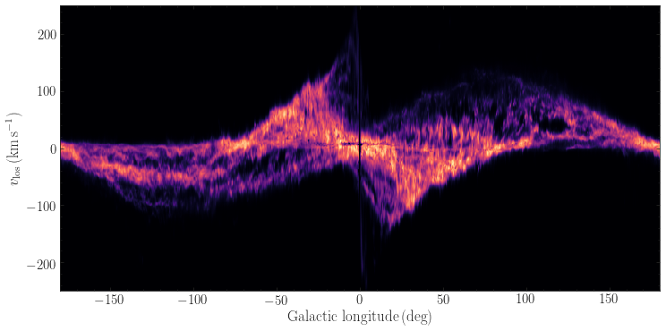
(Created using data from the HI4PI survey [HI4PI Collaboration et al. 2016]; because creating this map requires one to download GBs of data, we do not provide the code, but this map is simply created by taking their pixels at \(b=0^\circ\). In detail \(v_{\mathrm{los}}\) is their \(v_{\mathrm{LSR}}\).)

Another one is the \((l,v_\mathrm{los})\) diagram of molecular gas, for which we can use the molecular-cloud catalog of Miville-Deschênes et al. (2017) that we already used in Chapter 2.2.2. Because we will use the molecular-gas \((l,v_\mathrm{los})\) diagram to compare to models below, we first implement some functions to (a) download the data from Vizier, (b) read the GMC catalog, and (c) plot the \((l,v)\) distribution of the GMCs. To download the data from Vizier, we use the function that we defined in Section 9.2.2 above to download a catalog from the Vizier service. Then we read the catalog using astropy and convert it to a convenient pandas format:

import os, os.path
from astropy.io import ascii
_CACHE_BASEDIR= os.path.join(os.getenv('HOME'),'.galaxiesbook','cache')
_CACHE_VIZIER_DIR= os.path.join(_CACHE_BASEDIR,'vizier')
_MIVILLE_VIZIER_NAME= 'J/ApJ/834/57'
def gmc_read(verbose=False):
    """
    NAME:
       gmc_read
    PURPOSE:
       read the Miville-Deschênes GMC catalog
    INPUT:
       verbose= (False) if True, be verbose
    OUTPUT:
       pandas dataframe
    HISTORY:
       2017-09-12 - Written - Bovy (UofT)
    """
    # Generate file path and name
    tPath= os.path.join(_CACHE_VIZIER_DIR,'cats',
                        *_MIVILLE_VIZIER_NAME.split('/'))
    filePath= os.path.join(tPath,'table1.dat.gz')
    readmePath= os.path.join(tPath,'ReadMe')
    # download the file
    if not os.path.exists(filePath[:-3]):
        vizier(_MIVILLE_VIZIER_NAME,filePath,readmePath,
               catalogname='table1.dat.gz',readmename='ReadMe')
    # Read with astropy, w/o the .gz
    table= ascii.read(filePath[:-3],readme=readmePath,format='cds')
    return table.to_pandas()

Next we write a function to plot the \((l,v)\) diagram, because we will re-use it below:

def gmc_plot_lv(**kwargs):
    data= gmc_read()
    data= data[numpy.fabs(data['GLAT']) < 2.]
    s= data['Area']*15.
    s[s>30.]= 30.
    c= 'k'
    out= pyplot.scatter(data['GLON'],data['Vcent'],s=s,c=c,
                        cmap='gist_yarg',alpha=0.1,**kwargs)
    pyplot.xlabel(r'$\mathrm{Galactic\ longitude}\,(\mathrm{deg})$')
    pyplot.ylabel(r'$v_{\mathrm{los}}\,(\mathrm{km\,s}^{-1})$')
    pyplot.xlim(185.,-185.)
    pyplot.ylim(-200.,200.)
    return out

and then we plot the molecular-gas \((l,v_\mathrm{los})\) diagram:

data= gmc_plot_lv()

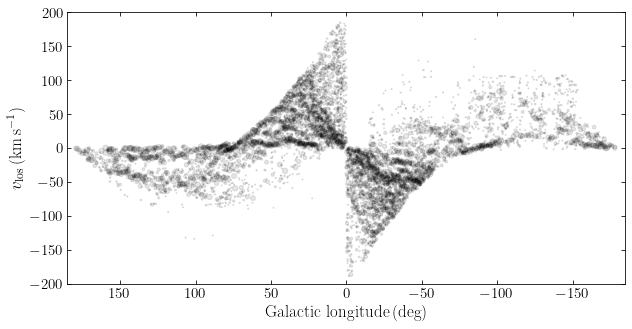
Both the HI and the molecular-gas \((l,v_\mathrm{los})\) diagrams display a similar pattern, with a similar envelope tracing the edges of the distribution and similar features near \(l=0^\circ\), but the intensity is different at different locations because the density distribution of neutral hydrogen and molecular gas is different (see Chapter 2.2.2).

These \((l,v_\mathrm{los})\) diagrams are thus full representations of the phase-space distribution of the interstellar medium. In the remainder of this section, we will discuss the mapping of the four-dimensional phase-space distribution \(f(R,\phi,v_R,v_\phi)\) (in polar coordinates) onto \((l,v_\mathrm{los})\). A minor complication that we will see is that at some locations in the \((l,v_\mathrm{los})\) diagram two different \((R,\phi,v_R,v_\phi)\) get projected onto the same \((l,v_\mathrm{los})\), so we can only recover \(f(R,\phi,v_R,v_\phi)\) up to this degeneracy.

9.3.2. Circular rotation and the longitude-velocity diagram

\label{sec-galrot-circlv}

We start by determining the patterns in the \((l,v_\mathrm{los})\) [which we will abbreviate as \((l,v)\) from hereon] diagram that we would see for a disk of gas in circular rotation with a rotation curve \(v_c(R)\). As usual, we will work in a left-handed Milky-Way frame where the disk rotates clockwise when seen from the North Galactic Pole. For a parcel of gas at a position \(\vec{x}\) with respect to the Galactic center that is on a circular orbit at radius \(R = |\vec{x}|\), the velocity is

\begin{equation} \vec{v} = \vec{v}_c(R)\times\hat{\vec{x}}\,, \end{equation}

where \(\vec{v}_c(R)\) is a vector with magnitude \(v_c(R)\) that is perpendicular to the mid-plane (pointing towards negative \(z\), so we can work out cross products with the usual right-hand rule) and \(\hat{\vec{x}}\) is the unit vector in the direction of \(\vec{x}\). We will assume that the observer itself is on a circular orbit at position \(\vec{x}_0\) with radius \(R=|\vec{x}_0|\) and velocity \(\vec{v}_0 = \vec{v}_c(R_0)\times\hat{\vec{x}}_0\); this orbit is called the local standard of rest (LSR) and we can approximately correct the Sun’s peculiar motion with respect to the LSR (which is about \(10\,\mathrm{km\,s}^{-1}\), although the exact value is still under debate; Chapter 11.3.1). The observed line-of-sight velocity \(v_\mathrm{los}\) is then the projection of the velocity difference \((\vec{v}-\vec{v}_0)\) onto the line-of-sight direction \((\vec{x}-\vec{x}_0)/|\vec{x}-\vec{x}_0|\)

\begin{align} v_\mathrm{los} & = (\vec{v}-\vec{v}_0)\cdot\frac{\vec{x}-\vec{x}_0}{|\vec{x}-\vec{x}_0|}\nonumber\\ & = \left(\vec{v}_c(R)\times\hat{\vec{x}}-\vec{v}_c(R_0)\times\hat{\vec{x}}_0\right)\cdot\frac{\vec{x}-\vec{x}_0}{|\vec{x}-\vec{x}_0|}\,. \end{align}

We can work this out further by expanding the dot product, writing \(\vec{v}_c(R) = \vec{\Omega}(R)\,R\), and using that \(\vec{a}\cdot(\vec{a}\times\vec{b}) = 0\) and \(\vec{a}\cdot(\vec{b}\times\vec{c}) = \vec{b}\cdot(\vec{c}\times\vec{a})\). We end up with

\begin{align} v_\mathrm{los} & = \left[\vec{\Omega}(R)-\vec{\Omega}(R_0)\right]\cdot\frac{\left(\vec{x}_0\times\vec{x}\right)}{|\vec{x}-\vec{x}_0|}\,. \end{align}

Using basic geometry, the last factor is equal to \(-R_0\,\sin l\,\hat{\vec{n}}\), where \(\hat{\vec{n}}\) is the unit vector perpendicular to the mid-plane pointing toward the North Galactic Pole. The rotation vector \(\vec{\Omega} = -|\vec{\Omega}|\,\hat{\vec{n}}\) and thus we get the final result

\begin{align}\label{eq-vlos-midplane-omega} v_\mathrm{los}(l) & = \left[\Omega(R)-\Omega(R_0)\right]\,R_0\,\sin l\,. \end{align}

This equation makes sense for the following reasons: (i) a disk in solid-body rotation has \(\Omega(R) = \mathrm{constant}\) and therefore \(v_\mathrm{los} = 0\) from Equation \(\eqref{eq-vlos-midplane-omega}\); this must be the case because in a disk in solid-body rotation, the distance between any two points remains constant and therefore there can be no non-zero line-of-sight velocities. Also, (ii) at \(l=0\) and \(l=180^\circ\), the line-of-sight velocity coincides with (minus) the Galactocentric radius velocity, which is zero for a disk in circular rotation; Equation \(\eqref{eq-vlos-midplane-omega}\) indeed gives \(v_\mathrm{los} = 0\) at \(l=0\) and \(l=180^\circ\). Finally, (iii) it is clear that the expression of \(v_\mathrm{los}(l)\) needs to involve the subtraction of the projection of the LSR motion onto the line of sight, which is \(-v_c(R_0)\,\sin l = -\Omega(R_0)\,R_0\,\sin l\); therefore \(R_0\sin l\) must multiply \(\left[\Omega(R)-\Omega(R_0)\right]\).

Let’s now explore how gas at different \((R,\phi)\) get mapped onto the \((l,v)\) plane using Equation \(\eqref{eq-vlos-midplane-omega}\) as our guide. Gas on a circular ring at radius \(R_c\) has a constant \(\Omega(R_c)\) along the ring (in the axisymmetric rotation approximation). Equation \(\eqref{eq-vlos-midplane-omega}\) therefore tells us that this ring will map onto a sinusoidal curve \(\propto \sin l\) with prefactor \(\left[\Omega(R_c)-\Omega(R_0)\right]\,R_0\). For \(R_c < R_0\), the ring does not subtend the entire longitude range, but runs from \(-\mathrm{arcsin}(R_c/R_0)\) to \(\mathrm{arcsin}(R_c/R_0)\). At \(R_c > R_0\), the ring subtends the entire range of Galactic longitudes.

If we then assume a rotation curve \(v_c(R)\), we can map any ring at \(R_c\) to a locus in the \((l,v)\) plane. In the following figure we do this for rings at a few different radii assuming a flat rotation curve (using galpy’s LogarithmicHaloPotential) and overlaying the locations of the rings on the map of the molecular clouds from Miville-Deschênes et al. (2017), using the function to plot this data that we defined above:

from galpy import potential
# Function to map (l,R) -> vlos
def vlos_ring(ls,Rc,pot=None,ro=8.):
    return (pot.omegac(Rc)-pot.omegac(ro))*ro*numpy.sin(ls)
figsize(10,5)
# First plot the GMCs
data= gmc_plot_lv()
ro= 8.*u.kpc
vo= 220.*u.km/u.s
lp= potential.LogarithmicHaloPotential(normalize=1.,
                                       vo=vo,ro=ro)
Rc= 3.*u.kpc
ls= numpy.linspace(-numpy.arcsin(Rc/ro),numpy.arcsin(Rc/ro),101)
line_3= plot(ls.to(u.deg),vlos_ring(ls,Rc,pot=lp,ro=ro).to(u.km/u.s),lw=3.,
            label=r'$R = %.0f\,\mathrm{kpc}$' % Rc.to(u.kpc).value)
Rc= 6.*u.kpc
ls= numpy.linspace(-numpy.arcsin(Rc/ro),numpy.arcsin(Rc/ro),101)
line_6= plot(ls.to(u.deg),vlos_ring(ls,Rc,pot=lp,ro=ro).to(u.km/u.s),lw=3.,
            label=r'$R = %.0f\,\mathrm{kpc}$' % Rc.to(u.kpc).value)
Rc= 12.*u.kpc
ls= numpy.linspace(-numpy.pi,numpy.pi,101)*u.rad
line_12= plot(ls.to(u.deg),vlos_ring(ls,Rc,pot=lp,ro=ro).to(u.km/u.s),lw=3.,
             label=r'$R = %.0f\,\mathrm{kpc}$' % Rc.to(u.kpc).value)
Rc= 20.*u.kpc
ls= numpy.linspace(-numpy.pi,numpy.pi,101)*u.rad
line_20= plot(ls.to(u.deg),vlos_ring(ls,Rc,pot=lp,ro=ro).to(u.km/u.s),lw=3.,
             label=r'$R = %.0f\,\mathrm{kpc}$' % Rc.to(u.kpc).value)
legend(handles=[line_3[0],line_6[0],
               line_12[0],line_20[0]],
       fontsize=18.,loc='upper left',frameon=False);

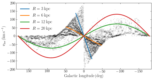
We see that the features which run from the top-left center of this figure to the bottom-right center arise from rings inside of the solar circle, \(R_c < R_0\). The material at negative \(v_\mathrm{los}\) for \(l >0\) (left side) and positive \(v_\mathrm{los}\) for \(l < 0\) (right side) comes from rings outside of the solar circle. Very few clouds are found outside of the red curve for \(R_c = 20\,\mathrm{kpc}\), indicating that very little molecular gas is located that far from the center.

The molecular-gas distribution has a strong overdensity that runs from the top-left center to the bottom-right center. It should now be clear that this is naturally explained if much molecular gas is found in a ring, somewhere between the blue and orange curve in the previous figure. A ring of \(R_c \approx 4.5\,\mathrm{kpc}\) provides a good match to the overdense feature (at least at positive \(l\)), as highlighted in the next figure:

figsize(10,5)
data= gmc_plot_lv()
Rc= 4.5*u.kpc
ls= numpy.linspace(-numpy.arcsin(Rc/ro),numpy.arcsin(Rc/ro),101)
line_4= plot(ls.to(u.deg),vlos_ring(ls,Rc,pot=lp,ro=ro).to(u.km/u.s),lw=3.,
            label=r'$R = %.1f\,\mathrm{kpc}$' % Rc.to(u.kpc).value)
legend(handles=[line_4[0]],
       fontsize=18.,loc='upper left',frameon=False);

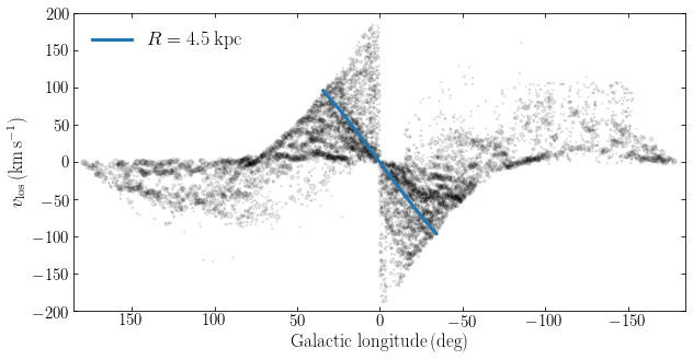
This indicates that there is an overdensity of molecular gas around \(R \approx 4.5\,\mathrm{kpc}\) in the Milky Way.

Coming back to galactic rotation, we can learn a few things from Equation \(\eqref{eq-vlos-midplane-omega}\). One is that the observed \(v_\mathrm{los}\) is only sensitive to \(\Omega(R)-\Omega(R_0)\), that is, differences in angular rotation rate. Adding a constant rotation rate \(\Omega_\mathrm{add}\) therefore does not change anything about the observed \((l,v)\) distribution. However, if we assume that as \(R \rightarrow \infty\) that \(\Omega(R) \rightarrow 0\), then Equation \(\eqref{eq-vlos-midplane-omega}\) tells us that \(v_\mathrm{los}(l) = -\Omega(R_0)\,R_0\,\sin l = -v_c(R_0)\,\sin l\) as \(R \rightarrow \infty\) and rings would bunch up near this “final” curve as we go to larger \(R\). Therefore, if we could measure the location of this final curve by delineating the outermost contour in the \((l,v)\) diagram, we could measure the circular velocity at the Sun’s location. The problem with this measurement is that it is difficult to see gas at large enough \(R\) for the limit \(R \rightarrow \infty\) to well describe the rotation curve. For example, for a flat rotation curve we have that \(\Omega(R) \propto \Omega(R_0)\,R_0/R\) and therefore for \(\Omega(R)\) to be, e.g., only 10% of \(\Omega(R_0)\), we require \(R = 10\,R_0 \approx 80\,\mathrm{kpc}\), where there is essentially no gas in the disk.

Therefore, to do this type of measurement of \(v_c(R_0)\) in the Milky Way, we require a model for the surface-density distribution \(\Sigma_{HI}(R)\) of the neutral hydrogen (we use neutral hydrogen, because CO has a shorter scale length than HI) and can then predict the amount of HI as a function of \(v_\mathrm{los}\) by mapping \(R \rightarrow v_\mathrm{los}\) using Equation \(\eqref{eq-vlos-midplane-omega}\). This was done by Knapp et al. (1978). Below, we display their Figures 9 and 10 which show the HI intensity toward \(l=90^\circ\) together with models for different values of \(v_c(R_0)\) (\(\Theta_0\) in their notation):

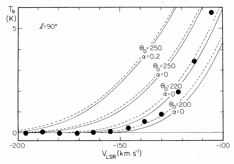
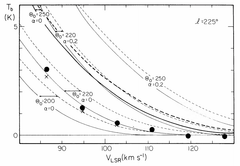
(Credit: Knapp et al. 1978)

We see that the intensity of HI emission (shown here as the brightness temperature \(T_b\)) agrees best with \(v_c(R_0) = 220\,\mathrm{km\,s}^{-1}\) in both of these directions. Based on this good agreement, this has been the standard value of \(v_c(R_0)\) for the last 35 years (Kerr & Lynden-Bell 1986). But the value of \(v_c(R_0)\) continues to be debated until this day and it is clear that this HI-based measurement is not unambiguous. Modern determinations of \(v_c(R_0)\) are made using, among others, the observed kinematics of disk stars based on dynamical-modeling techniques that we introduced in the next few chapters or using modeling of tracers in the stellar halo along the lines that we discussed in Part I.

The most important property of Equation \(\eqref{eq-vlos-midplane-omega}\) is that for rings inside the solar circle, the \((l,v)\) distribution terminates at a positive velocity for \(l > 0\) and a negative value for \(l < 0\). This terminal point at a given \(l\) is where a ring of radius \(R_c = R_0\,|\sin l|\) reaches its extremum in \(l\). At that point, \(v_\mathrm{los}\) is

\begin{equation}\label{eq-vterm} v_\mathrm{los, term}(l\in[-90^\circ,90^\circ]) = \left[\Omega(R_0\,|\sin l|)-\Omega(R_0)\right]\,R_0\,\sin l\,. \end{equation}

Because this is the locus on which the \((l,v)\) diagram ends or “terminates”, this is known as the terminal velocity curve. Because the terminal velocity is that along the line of sight where the line of sight is tangent to the circle with \(R_c = R_0\,|\sin l|\), this method is also known as the tangent-point method. We can measure the terminal velocity as a function of \(l\) by delineating the line at which the \((l,v)\) distribution ends (because the terminal-velocity curve is made up of gas inside of the solar circle, there is no reason to think that there would be no gas observed at this terminal curve, which is different from the “final curve” at large \(R\) that we discussed above). With measurements of \(v_\mathrm{los, term}(l)\) in hand, we can then determine the rotation curve from Equation \(\eqref{eq-vterm}\)

\begin{equation}\label{eq-vterm-vc} v_c(R) = \pm v_\mathrm{los, term}(l) + v_c(R_0)\,\frac{R}{R_0}\,, \end{equation}

where \(l = \pm\mathrm{arcsin}(R/R_0)\). Each value of \(|l|\) gives two independent estimates of \(v_c(R)\). Equation \(\eqref{eq-vterm-vc}\) is one of the main methods with which the Milky Way’s rotation curve has been determined at \(R < R_0\).

We can directly compare the terminal velocity curve for different potentials with the observed \((l,v)\) distribution. In the following figure we do this for three rotation curve: a flat rotation curve \(v_c(R) = \mathrm{constant}\), a solid-body rotation curve \(v_c(R) = \Omega\,R\), and the rotation curve for a razor-thin exponential disk with \(R_d = 3\,\mathrm{kpc}\). We use \(v_c(R_0) = 220\,\mathrm{km\,s}^{-1}\) for all three rotation curves. This predicts the following terminal-velocity curves using Equation \(\eqref{eq-vterm}\):

figsize(10,5)
data= gmc_plot_lv()
ylim(-225.,225.)
ro= 8.*u.kpc
vo= 220.*u.km/u.s
lp= potential.LogarithmicHaloPotential(normalize=1.,
                                       vo=vo,ro=ro)
ls= numpy.linspace(-numpy.pi/2.,numpy.pi/2.,101)*u.rad
line_flat= plot(ls.to(u.deg),lp.vterm(ls).to(u.km/u.s),lw=3.,
               label=r'$v_c(R) = \mathrm{constant}$')
# size R of homogeneous >> considered region
hp= potential.HomogeneousSpherePotential(normalize=1.,R=10.,
                                         vo=vo,ro=ro)
line_solid= plot(ls.to(u.deg),
                 u.Quantity([hp.vterm(l).to(u.km/u.s) for l in ls]),
                 lw=3.,
                 label=r'$\Omega(R) = \mathrm{constant}$')
rp= potential.RazorThinExponentialDiskPotential(normalize=1.,
                                                hr=3.*u.kpc,
                                               vo=vo,ro=ro)
ls= numpy.linspace(0.,numpy.pi/2.,101)*u.rad
line_rp= plot(ls.to(u.deg),rp.vterm(ls).to(u.km/u.s),lw=3.,
             label=r'$v_c(R) = \mathrm{exp.\ disk}$')
plot(-ls.to(u.deg),-rp.vterm(ls).to(u.km/u.s),lw=3.,
     color=line_rp[0].get_color())
legend(handles=[line_flat[0],line_solid[0],
               line_rp[0]],
       fontsize=18.,loc='upper left',frameon=False);

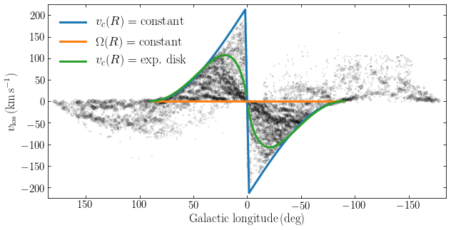
As expected, the solid-body rotation curve is zero everywhere (remember that solid-body rotation keeps all relative line-of-sight velocities zero within a disk) and it is clear that gas in the Milky Way does not rotate as a solid body. The terminal velocity curve from the razor-thin exponential disk turns over around \(l=20^\circ\), which is not observed in the distribution. The terminal velocity curve of a flat rotation curve rises toward \(l=0\) (from the side of positive \(l\)) in a similar way as observed in the data. We should not overinterpret this good agreement, because it is somewhat accidental: within \(\approx R_0\,\sin 30^\circ = 4\,\mathrm{kpc}\), the bar dominates the potential and gas is not on circular orbits as we assumed in the derivation so far, so we cannot directly interpret the observed terminal velocity curve at \(|\sin l| < 1/2\) in terms of the rotation curve of an axisymmetric disk (e.g., Chemin et al. 2015).

So far we have only discussed the effect of axisymmetric galactic rotation on the observed \((l,v)\) diagram. Looking more closely at the \((l,v)\) diagrams of HI and of the molecular gas, we see that there are significant overdensities in it. We have explained one of these as the signature of a ring of molecular gas, but others cannot be interpreted in terms of rings and even the ring that we purportedly explained looks distinctly asymmetric in \(l\).

9.4. Observing differential rotation locally: The Oort constants

\label{sec-galrot-oort}

So far, we have discussed galactic rotation in external galaxies and over the full extent of the Milky Way using observations of the kinematics of the interstellar medium, but historically the first evidence that the Milky Way is not rotating as a solid body—hence differential rotation—came from the kinematics of nearby stars. One might think that the motions of nearby stars would only be negligibly affected by the overall rotation of the disk, but in fact the differential rotation of the Milky Way is apparent in the motions of stars within just a few 100 pc. Because it remains important in a variety of astrophysical contexts (e.g., in accretion disks: Balbus & Hawley 1991; Balbus & Hawley 1992), we briefly go over the formalism describing the local dynamics of a differentially-rotating disk and its application to the local velocity field.

We consider the velocity field of a stellar population in the mid-plane of the Galaxy; the velocity field is given by the average velocity \(\langle \vec{v}\rangle(R,\phi)\) as a function of position in the Milky Way. This leaves aside, for now, the question of whether this velocity field is that of an axisymmetric galaxy and whether the mean rotational velocity is the circular velocity \(v_c(R)\). The latter of these turns out to be a quite subtle question that we will only resolve in Chapter 11.

Consider the rectangular Galactic coordinate system \(\vec{X} = (X,Y)\) centered on the Sun introduced in Appendix A.2. We work at \(b = 0\) and therefore \(X = D\,\cos l\) and \(Y = D\,\sin l\), where \(D\) is the distance. Using the distance \(R_0\) to the Galactic center, we can convert between Galactic \((X,Y)\) coordinates and Galactocentric \((R,\phi)\) coordinates; in particular we can consider the mean velocity field as a function of \((X,Y)\): \(\langle \vec{v}\rangle(X,Y)\). We can Taylor expand the velocity field around the Sun’s position \((X,Y) = (0,0)\) as (to simplify notation, we will denote partial derivatives evaluated at \((X,Y) = (0,0)\) as follows: \(\frac{\partial f_x}{\partial x}\Big|_{(0,0)} \equiv f_{x,x}\))

\begin{equation} \langle \vec{v}\rangle(X,Y) = \langle \vec{v}\rangle(0,0)+\,\left(\begin{matrix} v_{X,X} & v_{X,Y} \\ v_{Y,X} & v_{Y,Y}\end{matrix}\right)\,\left(\begin{matrix} X\\Y\end{matrix}\right)\,, \end{equation}

where \((v_X,v_Y)\) are the \(X\) and \(Y\) components of the mean velocity field. The difference between the mean velocity and the mean velocity at the Sun is then given by

\begin{equation}\label{eq-dvmean-matrix} \delta\langle \vec{v}\rangle(X,Y) = \langle \vec{v}\rangle(X,Y) - \langle \vec{v}\rangle(0,0)= \,\left(\begin{matrix} K+C & A-B \\ A+B & K-C\end{matrix}\right)\,\left(\begin{matrix} X\\Y\end{matrix}\right)\,, \end{equation}

where we have also introduced an alternative way to write the partial derivatives in the matrix.

The observed line-of-sight velocity \(v_\mathrm{los}\) of a nearby star at \(b=0\) is the combination of (i) the mean difference given in Equation \(\eqref{eq-dvmean-matrix}\), (ii) the Sun’s motion \(\vec{v}_\odot = (U_0,V_0)\) with respect to \(\langle \vec{v}\rangle(0,0)\), and (iii) random motions. We will ignore the random component and obtain the line-of-sight velocity \(v_\mathrm{los}(D,l)\) at a given distance \(D\) and longitude \(l\) by projecting the full velocity onto the line of sight

\begin{align} v_\mathrm{los}(D,l) & = \hat{\vec{X}}\cdot \left[\delta\langle \vec{v}\rangle-\vec{v}_\odot\right]\nonumber\\ & = \frac{1}{D}\left(\begin{matrix} X & Y \end{matrix}\right)\, \left[\left(\begin{matrix} K+C & A-B \\ A+B & K-C\end{matrix}\right)\,\left(\begin{matrix} X\\Y\end{matrix}\right)-\left(\begin{matrix} U_0\\V_0\end{matrix}\right)\right]\nonumber\\ & = D\,\left[K + A\,\sin 2l + C\,\cos 2l\right]-U_0\,\cos l - V_0\,\sin l\,,\label{eq-oort-vlos} \end{align}

where we used the trigonometric relations \(2\sin l\,\cos l = \sin 2l\) and \(\cos^2 l-\sin^2 l = \cos2l\). We can derive a similar relation for the proper motion \(\mu_l(D,l)\)

\begin{align} \mu_l(D,l) & = \frac{1}{D}\,\left(\hat{\vec{X}}\times \left[\delta\langle \vec{v}\rangle-\vec{v}_\odot\right]\right)_z\nonumber\\ & = \frac{1}{D}\,\left(X\,\left[\delta\langle \vec{v}\rangle-\vec{v}_\odot\right]_y - Y\left[\delta\langle \vec{v}\rangle-\vec{v}_\odot\right]_x\right)\nonumber\\ & = B + A\,\cos 2l - C\,\sin 2l+\frac{1}{D}\left[U_0\,\sin l - V_0\,\cos l\right]\,,\label{eq-oort-pm} \end{align}

where we obtained the tangential velocity in the first line as the \(Z\) component of the cross product of the position vector and the relative velocity (which picks out the component perpendicular to the line of sight).

Equations \(\eqref{eq-oort-vlos}\) and \(\eqref{eq-oort-pm}\) demonstrate that if we can measure the pattern of radial velocities and proper motions of stars, we can determine the quantities \((A,B,C,K)\). Because these quantities come in as either a constant term (\(K\) and \(B\)) or a sine or cosine of \(2l\), while the Sun’s motion contributes a sine or cosine of \(l\), with full longitude coverage we can separate the contribution from the Sun’s motion from that from the derivative of the mean velocity field.

Let us now consider these constants for a population of stars believed to be on average on circular orbits in an axisymmetric disk. In this case, the quantities \((A,B,C,K)\) are known as the Oort constants. Oort (1927) presented the first measurement of these. For circular orbits in an axisymmetric disk, the mean radial velocity is zero and at the Sun’s location \(v_X = -v_R\), where \(v_R\) denotes the Galactocentric radial component of the mean velocity. We also have that \(X = R_0-R\) for points at \(Y=0\); therefore we must have that \(v_{X,X} = 0\) or \(K+C = 0\). Similarly, \(v_Y = v_c(R)\) at the Sun’s location and the \(Y\) axis is tangential to a circular orbit at \(X=0\). Along the tangential direction, \(v_c(R)\) does not change in an axisymmetric disk, and therefore \(v_{Y,Y} = 0\) or \(K-C = 0\). It must therefore be the case that \(K = C = 0\) in an axisymmetric disk.

What about \(A\) and \(B\)? Again, \(v_Y = v_c(R)\) and \(X = R_0 - R\), so it must be the case that \(v_{Y,X} = -\mathrm{d} v_c(R) / \mathrm{d} R\) or that

\begin{equation}\label{eq-oort-apb} A+B = -\frac{\mathrm{d} v_c(R)}{\mathrm{d} R}\Bigg|_{R=R_0}\,. \end{equation}

The final relation for \(v_{X,Y}\) is a little trickier. To determine this, we need \(v_X = v_c(R)\,y/\sqrt{y^2+(R_0-x)^2}\), which holds in an axisymmetric galaxy. Then \(v_{X,Y} = v_c(R) / R_0\) or

\begin{equation}\label{eq-oort-amb} A-B = \frac{v_c(R_0)}{R_0}\,. \end{equation}

The relations in Equations \(\eqref{eq-oort-apb}\) and \(\eqref{eq-oort-apb}\) relate the Oort constants \(A\) and \(B\) to the rotation curve in an axisymmetric disk. Re-arranging them we have that

\begin{align} 2A & = \phantom{-}\frac{v_c(R_0)}{R_0}-\frac{\mathrm{d} v_c(R)}{\mathrm{d} R}\Bigg|_{R=R_0}\,,\\ 2B & = -\frac{v_c(R_0)}{R_0}-\frac{\mathrm{d} v_c(R)}{\mathrm{d} R}\Bigg|_{R=R_0}\,.\label{eq-oort-b} \end{align}

Another way to write \(A\) is as

\begin{equation}\label{eq-oort-a-domega} 2A = -R_0\,\frac{\mathrm{d} \Omega(R)}{\mathrm{d} R}\Bigg|_{R=R_0}\,, \end{equation}

where \(\Omega(R)\) is the angular rotation rate of the disk. Therefore, \(A\) would be zero if the disk were in solid-body rotation and because the differential rotation of non-solid-body rotation shears the disk, \(A\) is known as the azimuthal shear. Oort was the first to measure \(A\) from the behavior of \(v_\mathrm{los}\) of local stars: for an axisymmetric disk and setting \((U_0,V_0) = (0,0)\) for simplicitly, Equation \(\eqref{eq-oort-vlos}\) becomes

\begin{equation} v_\mathrm{los}(D,l)= D\,A\,\sin 2l\,, \end{equation}

and the line-of-sight velocities should therefore display a simple sinusoidal pattern for stars at a given distance \(D\). This expression also makes sense in light of the discussion of the line-of-sight velocity field of the interstellar medium above: a solid-body rotation disk has zero relative line-of-sight velocities everywhere, so must have \(A=0\). Oort (1927) measured \(A\) from the line-of-sight velocities and found that it was \(A\approx 31\,\mathrm{km\,s}^{-1}\,\mathrm{kpc}^{-1}\) (with a rather small uncertainty of \(\approx3\,\mathrm{km\,s}^{-1}\,\mathrm{kpc}^{-1}\)!). This value was significantly different from zero, indicating that the disk does not rotate as a solid body and providing the first evidence of the differential rotation of the Milky Way disk. As we will discuss below, this value is however significantly different from that found by modern determinations.

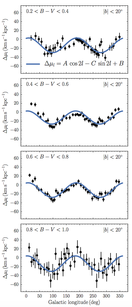
The first data release from Gaia, an astrometric space mission measuring parallaxes and proper motions for millions of stars, has provided us with a sample of proper motions for hundreds of thousands of stars within a few hundred parsec (Gaia Collaboration et al. 2016a; Gaia Collaboration et al. 2016b). These allow one to measure \(A\), \(B\), and \(C\) using Equation \(\eqref{eq-oort-pm}\). The inverse distance that is required in the terms for the Sun’s motion is given by the observed parallax. Bovy (2017a) has performed this measured for different stellar types. The following figure shows the mean proper motion \(\mu_l(l)\) after correcting for the best-fit solar motion \((U_0,V_0)\) using the parallax for each star:

(Credit: Bovy 2017a)

This figure beautifully displays the dominant \(\cos 2l\) behavior expected from Equation \(\eqref{eq-oort-pm}\) for a close-to-axisymmetric disk (\(C \approx 0\) and therefore the \(\sin 2l\) term is sub-dominant). The overall offset from zero is \(B\). From these figures it should be clear that \(A \approx -B \approx 15\,\mathrm{km\,s}^{-1}\,\mathrm{kpc}^{-1}\). A detailed fit gives

\begin{align}\label{eq-galrot-obsOort-A} A & = \phantom{-}15.3 \pm 0.4 \,\mathrm{km\,s}^{-1}\,\mathrm{kpc}^{-1}\,,\\ B & = -11.9 \pm 0.4 \,\mathrm{km\,s}^{-1}\,\mathrm{kpc}^{-1}\,,\label{eq-galrot-obsOort-B}\\ C & = -\phantom{1}3.2 \pm 0.4\,\mathrm{km\,s}^{-1}\,\mathrm{kpc}^{-1}\,,\\ K & = -\phantom{1}3.3\pm 0.6\,\mathrm{km\,s}^{-1}\,\mathrm{kpc}^{-1}\,.\label{eq-galrot-obsOort-K} \end{align}

All of these were determined from observations of the proper motions alone. This makes use of the fact that if we assume that the disk is in cylindrical rotation then Equation \(\eqref{eq-oort-vlos}\) applies to the component of the line-of-sight velocity that is parallel to the mid-plane. But for \(b \neq 0\), the actual line-of-sight velocity is directed away from the mid-plane and the cylindrical radial velocity gets mixed into the line-of-sight velocity as well as the \(b\) component of the proper motion in the observational spherical coordinate system. This leads to an equation for \(\mu_b(l)\) similar to Equation \(\eqref{eq-oort-pm}\)

\begin{align}\label{eq-oort-pmb-b} \mu_b(D,l) = -& \left( K + A\,\sin 2l + C\,\cos 2l\right)\,\sin b\,\cos b\\ & +\frac{1}{D}\left[\left(U_0\,\cos l + V_0\,\sin l\right)\,\sin b - W_0 \cos b\right]\,,\nonumber \end{align}

where we have now explicitly included the \(b\) dependence and \(W_0\) is the Sun’s motion vertically with respect to the plane. Therefore, we can use observations of \(\mu_b(l)\) to determine \(A\), \(C\), and \(K\) and combine them with the \(A\), \(B\), and \(C\) measurements from \(\mu_l(l)\) to determine all four Oort constants. For completeness and for use in Chapter 11, we also state the equations for \(v_\mathrm{los}(D,l)\) and \(\mu_l(D,l)\) that include the \(b\) dependence

\begin{align}\label{eq-oort-vlos-b} v_\mathrm{los}(D,l) & = D\,\left[K + A\,\sin 2l + C\,\cos 2l\right]\,\cos b\\ & \quad -\left(U_0\,\cos l + V_0\,\sin l\right)\cos b + W_0\,\sin b\,,\nonumber\\ \mu_l(D,l) & = \left(B + A\,\cos 2l - C\,\sin 2l\right)\,\cos b+\frac{1}{D}\left[U_0\,\sin l - V_0\,\cos l\right]\,.\label{eq-oort-pm-b} \end{align}

The measurements of the Oort constants indicate that (i) the rotation curve is slightly declining at the Solar circle, with \(\mathrm{d}v_c(R) / \mathrm{d} R \approx -3\,\mathrm{km\,s}^{-1}\,\mathrm{kpc}^{-1}\), (ii) the angular rotation rate is \(\Omega(R_0) \approx 27\,\mathrm{km\,s}^{-1}\,\mathrm{kpc}^{-1}\), in good agreement with the standard values of \(v_c(R_0) = 220\,\mathrm{km\,s}^{-1}\) and \(R_0 = 8\,\mathrm{kpc}\), which give \(v_c(R_0) / R_0 = 27.5\,\mathrm{km\,s}^{-1}\,\mathrm{kpc}^{-1}\), and (iii) the disk is non-axisymmetric because both \(C\) and \(K\) are significantly different from zero; however, non-axisymmetry can be largely treated as a perturbation near the Sun, because \(|C|/(A-B)\) and \(|K|/(A-B) \ll 1\).

To interpret the measurements discussed here in terms of the rotation curve, we have assumed that the observed stars on average travel on circular (or at least closed in the case of non-axisymmetry) orbits. We will see in the next chapter that this is in fact not the case: In typical disks, the average rotation velocity of a sample of stars at a given radius is less than the circular velocity at that radius. However, the effect of this on the Oort constants \(A\) and \(B\) is small—less than \(\approx 1\,\mathrm{km\,s}^{-1}\,\mathrm{kpc}^{-1}\) (Bovy 2015)—so the mean-field kinematics of nearby stars provides rather accurate measurements of the Oort constants and Galactic rotation in the Milky Way.