
3. Gravitation
In this chapter, we introduce the basics of gravitational dynamics: how does mass give rise to forces that lead to the motion of planets, stars, gas, and dark matter in the Universe? The next chapters discuss how masses move under the influence of the gravitational force—these motions we refer to as “orbits”—which is the realm of classical mechanics, and we introduce the important concept of dynamical equilibrium.
In this first part, we apply these concepts to mass distributions that are spherically symmetric. Real galaxies look like this:
|
|
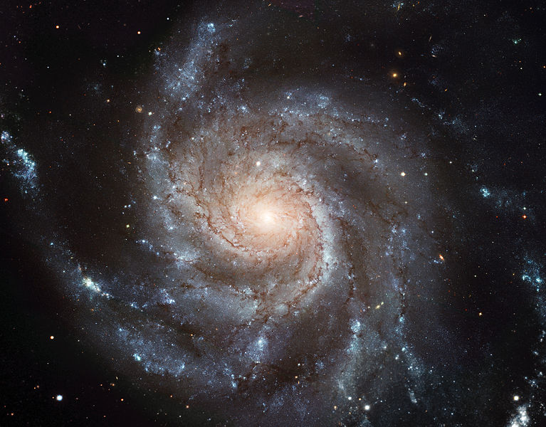
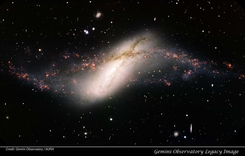
(Credit: M101: European Space Agency & NASA; NGC 660: Gemini Observatory, AURA)
One might therefore wonder how useful it is to study spherical mass distributions, when most galaxies are so far from being spherically symmetric. We will see in later chapters that, even though mass distributions can be quite far from spherical, many of the properties of non-spherical distributions can be understood by approximating these distributions with some equivalent spherical distribution. Similarly, many of the concepts that we will introduce in this chapter (like that of dynamical time and the circular velocity) remain similar for non-spherical distributions. And spherical mass distributions provide a simple manner to introduce many of the concepts that are relevant for all galaxies.
3.1. Matter and the gravitational field
A theory for the motion of objects under the influence of gravity requires two ingredients: how mass gives rise to a gravitational force and how objects move under the influence of this force. In classical physics, the laws for each of these go back to Newton and contemporaries: Newton’s law of universal gravitation that gives the force \(F\) from a mass \(M\) acting on a second mass \(m\) in terms of the distance \(r\) between the two as \(F = -GMm/r^2\), and Newton’s second law that gives the relation between force and acceleration \(a\) for an object with mass \(m\) as \(F = ma\). A more modern understanding of the law of universal gravitation, however, emphasizes that the three-dimensional force \(\vec{F}(\vec{x})\) derives from a scalar-valued gravitational potential \(\Phi(\vec{x})\) through:
and replaces Newton’s inverse-square law of gravitation with the Poisson equation as the fundamental equation relating mass and gravitational force:
where \(\rho(\vec{x})\) is the mass density, \(G\) is the gravitational constant, and \(\nabla^2\) is the Laplace operator.
The reason that the Poisson equation is more properly considered to be the fundamental equation between mass and gravitational force is that it is the direct Newtonian limit of Einstein’s field equation \(R_{\mu\nu} -R\,g_{\mu\nu}/2 = 8\pi G\,T_{\mu\nu}\) in the general theory of relativity, which is our best theory of gravity so far. This is not a book about the general theory of relativity and the origin of Einstein’s field equation is typically not important for understanding galaxy dynamics, but a key point is that Einstein’s field equation reduces to the Poisson equation in the limit that velocities \(v\) and the gravitational potential are small compared to the speed of light \(c\) (the potential \(\Phi\) has units of velocity squared, so this limit is \(|\Phi|/c^2 \ll 1\) and \(v/c\ll 1\)). This limit always applies on the scale of galaxies, with the notable exception of gravitational lensing by galaxies as discussed in Chapter 16. For the interested reader, Appendix C has a self-contained discussion of Einstein’s field equation and how it reduces to the Poisson equation in the low-velocity limit.
Before continuing our discussion, it is worth noting that the Poisson equation (or its generalization, Einstein’s field equation) is a hypothesis. Like any other physical theory, we test the Poisson equation by making predictions derived using this equation and testing these predictions against observational data. Gravity as defined by the Poisson equation is extraordinarily well tested using laboratory experiments and solar-system gravitational dynamics: it is known to hold to one-part-in-one-billion in these settings (Adelberger et al. 2003; Will 2014). Partly because of these tests, most astrophysicists assume that the Poisson equation holds on the scales of galaxies and on the scale of the Universe (as Einstein’s equation) and that any anomalies that may result from its application are due to new forms of mass or energy that enter the mass density \(\rho\) or the energy-momentum tensor \(T_{\mu\nu}\), rather than indicating a problem with the Poisson equation. Large anomalies are indeed known to exist: these are dark matter, which is a \(\approx100\%\) anomaly on the scales of galaxies, and dark energy, which is a \(\approx100\%\) anomaly on the largest cosmological scales (meaning that ignoring them leads to \(\mathcal{O}(1)\) discrepancies with the observations).
Throughout this book, we will largely assume that the Poisson equation holds and, thus, that dark matter (and dark energy, but it is less important for our purposes) is a new form of matter whose density distribution can be studied using the Poisson equation. Theories that attempt to account for the anomalies typically interpreted as dark matter and dark energy without introducing new forms of matter and energy do so by modifying the Poisson equation or Einstein’s equation. Such modifications have to account for the fact that the Poisson equation holds to high accuracy in the solar system and, thus, can only change the Poisson equation in vastly different physical regimes.
Starting from the Poisson equation, we can derive Newton’s inverse-square law by computing the gravitational potential for a point mass \(M\) at position \(\vec{x}\). Because the Laplacian is a differential operator, we can move the origin of the coordinate system to any position, and calculations are most straightforward if we position the mass at the origin. The density in this case is \(\propto\delta(\vec{x})\), where \(\delta(\cdot)\) is Dirac’s delta function (Chapter B.1.1) . To show that the potential \(\Phi(\vec{x}) = -GM/r\), where \(r = |\vec{x}|\), is the solution of the Poisson equation in this case, we compute the Laplacian of \(-GM/r\) for \(r \neq 0\) using the expression for the Laplacian in spherical coordinates (Equation A.12):
Thus, the density is zero for all \(r\neq 0\). Finally, to show that at \(r=0\), the density corresponding to \(\Phi(\vec{x}) = -GM/r\) is the correct delta function, we integrate the Laplacian of \(\Phi/(4\pi G)\) over a small spherical volume \(V\) of radius \(R\) with surface \(S\), because this should equal the mass \(M\):
Here, we have used the divergence theorem in going to the second line and the expression for the gradient in spherical coordinates in going to the third line (Equation A.11); \(\vec{\hat{r}}\) is the unit vector in the radial direction, which is perpendicular to the surface \(S\). Thus, the gravitational potential of a point mass \(M\) at distance \(r\) is \(\Phi = -GM/r\). Using that the gravitational force is the gradient of the potential from Equation \(\eqref{eq-force-gradient-potential}\), we find Newton’s law of gravity: at a three-dimensional position \(\vec{x}\) a distance \(r\) from the point-mass \(m\)
Putting the position \(\vec{x}_0\) of the mass \(M\) back in explicitly, this force law becomes
where we have used the standard simplification that the unit vector along \((\vec{x}-\vec{x}_0)\) is \((\vec{x}-\vec{x}_0)/|\vec{x}-\vec{x}_0|\). Because the force falls off as \(1/r^2\) rather than following something like a fast exponential decline, it is called a long-range force. In particular, if a point mass \(m\) is surrounded by a density of point masses that is uniform, then the amount of mass \(M\) in a shell at distance \(R\) is \(\propto R^2\), which combined with the \(1/R^2\) behavior of the force means that the force acting on \(m\) from shells at different \(R\) is approximately constant. In a constant-density medium, there are many more such shells at large distances than at small distances, and therefore the force is dominated by the total contribution from distant shells, rather than that from a few nearby shells.
A pair of functions (\(\Phi,\rho\)) that solve the Poisson equation \((\nabla^2 \Phi = 4\pi G \rho)\) is known as a potential-density pair. Because the Laplacian is a linear differential operator, we have that a linear combination of solutions to the Poisson equation is itself a solution: for potential-density pairs (\(\Phi_1,\rho_1\)) and (\(\Phi_2,\rho_2\)), the pair (\(\Phi_1+\Phi_2,\rho_1+\rho_2\)) is also a solution. A consequence of this is that the gravitational potential for a set of \(N\) point masses is simply given by the sum of the potentials for the individual point masses: If an object at \(\vec{x}\) with mass \(m\) is at a distance \(d_i = |\vec{x}-\vec{x}_i|\) from point masses \(M_i\) at positions \(\vec{x}_i\), the total gravitational potential is
Similarly, the gravitational force is
Note that this follows directly from the Poisson equation, while deriving it from Newton’s law of universal gravitation would require the additional assumption that forces add up linearly (which is of course baked into the Poisson equation).
The mass of galaxies is contained in discrete chunks, whether they be stars, putative dark-matter particles, or the atoms and molecules of the interstellar medium. Even though this matter is discrete, the overall distribution of mass is rather uniform, and the gravitational force even between large chunks like stars is therefore dominated by distant bodies (see the argument above). Therefore, we can approximate the density in a galaxy as a smooth function, rather than as a sum over discrete bodies. From the Poisson equation, this means that the gravitational potential and gravitational force are smooth functions as well: Because the density is a second derivative of the potential, the potential is essentially a double integral of the density and, therefore, much smoother than the density.
Newton’s second law (which will be discussed in more detail in the next chapter), states that mass times acceleration equals force. The mass that appears in this equation is the same mass as that appears in the equation between the gravitational potential and force (Equation [\(\ref{eq-force-gradient-potential}\)]; or in Newton’s law of gravitation if you wish). Therefore, we have that
or
The motion of an object in a smooth, external gravitational potential therefore does not depend on its mass. This fails when the field is not external, that is, when the object’s mass has an effect on its surrounding mass distribution, which in turn affects its motion through Newton’s second law. But for many applications of galaxy dynamics, a smooth, external gravitational potential is an excellent approximation. It therefore makes sense to introduce the gravitational field \(\vec{g}(\vec{x})\)—the force per unit mass— as
because then in a smooth, external potential we have that
This is known as the weak equivalence principle or the universality of free fall: all objects fall the same in an external gravitational field, whether they be feathers, stones, or stars. Einstein made this principle the centerpiece of his theory of relativity.
Because most of the time we do not need to consider an object’s mass to discuss its motion under gravity, we typically deal only with the gravitational field and much of the literature on galactic dynamics uses the terms “gravitational force” and “gravitational field” interchangeably and often uses the force symbol \(\vec{F}\) when really the field \(\vec{g}\) is meant. In this book, I will attempt to correctly use the terms “force” and “field”. Similarly, because of the weak equivalence principle, the gravitational field and the acceleration caused by it are the same, and the terms acceleration and force/field are often used interchangeably. Obviously we can only do this when the force is that due to gravity.
When working with physical quantities and equations, it is often useful to keep their units in mind. From the universality of free fall, we know that the units of gravitational field are the same as those of acceleration: length over time squared. The gravitational field is the spatial derivative of the gravitational potential. Therefore, gravitational potential has units of length squared over time squared, or more simply, velocity squared. Conversely, from the Poisson equation, we have that \(G\times\mathrm{density}\) has the same units as the spatial derivative of the gravitational field: units of inverse-time squared. \(G\) itself therefore has units of length cubed over mass over time squared. For galactic systems, \(G\) is most usefully expressed as (using the CODATA 2018 version of the recommended values of the fundamental physical constants)
where \(M_\odot\) is the mass of the Sun. We can also write this as
Because gravity is such a weak force, measuring \(G\) precisely is difficult and the relative uncertainty of the current measurement is \(2\times 10^{-5}\). This is a much larger relative uncertainty than those of other physical constants, which have typical relative uncertainties of \(\approx 10^{-10}\). However, essentially all of astrophysics is only sensitive to the combination \(GM_\odot\), which is known to a relative uncertainty of \(\approx 10^{-10}\), because it is measured using the orbits of spacecraft in the solar system. It is worth remembering that whenever you see a quoted measured mass outside of the solar system, what is really determined is \(G\) times that mass.
To sum up: The Poisson equation is the fundamental equation one has to solve to obtain the gravitational force due to any mass distribution. Because of this fundamental relation, we will use the terms mass distribution and (gravitational) potential interchangeably (where “gravitational” is typically implied in this context if it is not mentioned in front of “potential”). The (negative) gradient of the potential gives the gravitational field that gives rise to motion and is therefore the only quantity that has physical significance. Thus, we can add or subtract any constant from the potential without changing the dynamics; whenever possible we shall fix this constant such that the potential equals zero at \(r = \infty\).
3.2. Spherical systems: Newton’s shell theorems
For spherical mass distributions, Newton proved two fundamental theorems that significantly simplify all work with spherical mass distributions and, in particular, that of solving the Poisson equation. These are:
Newton’s first shell theorem: A body that is inside a spherical shell of matter experiences no net gravitational force from that shell.
Newton’s second shell theorem: The gravitational force on a body that lies outside a spherical shell of matter is the same as it would be if all of the shell’s matter were concentrated into a point at its center.
A direct, mathematical proof is most easily based on Gauss’s theorem, which is a direct consequence of the Poisson equation. Let’s integrate the Poisson equation over an arbitrary volume \(V\) containing total mass \(M\) and bounded by the surface \(S\) and use the divergence theorem to turn the volume integral into a surface integral. Then we obtain that
where \(\vec{\hat{n}}\) is the unit vector perpendicular to the surface \(S\). Thus, the integral of the component of the gravitational field perpendicular to a given surface is equal to the mass contained within that surface (multiplied by \(-4\pi G\)).
To prove Newton’s first shell theorem, we consider a spherical shell \(S_a\) centered on the origin with radius \(a\) and we integrate the gravitational field over a similar spherical shell \(S_b\) with radius \(b < a\). By symmetry, the gravitational field can only depend on \(r\) and for a non-zero field would therefore be constant \(g_b\) on \(S_b\); its integral over \(S_b\) is therefore \(4\pi b^2 \,g_b\)—the surface of the shell times the gravitational field. By Gauss’ theorem, this should equal \(-4\pi\,G\) times the enclosed mass, which is zero because \(S_b\) is within \(S_a\). Therefore, the gravitational field \(g_b = 0\). This holds for all \(b < a\), which proves Newton’s first shell theorem.
Newton’s second shell theorem can be proven in a similar way. We now integrate over a shell \(S_c\) with \(c > a\). Again, the gravitational field on this shell is a constant \(g_c\) and the integral is equal to \(4\pi c^2 g_c\). Because \(S_c\) is outside of \(S_a\), all of \(S_a\)’s mass is contained within \(S_c\) and Gauss’ theorem now implies that this should equal \(-4\pi\,G\) times the mass of the shell \(S_a\). Because this equality does not depend on the radius \(a\) of \(S_a\), it would be the same if we shrunk the shell to a point, thus proving Newton’s second shell theorem.
Newton originally proved his first shell theorem using more geometric means that are more intuitive. We consider the force on a point interior to a thin shell from a small section of the shell obtained from the two intersections of a cone centered on this point with a small opening angle as in the following figure:
[6]:
figsize(6,6)
gca().add_patch(Circle((0.2,0.1),radius=1,fc='none',ec='k',zorder=0))
gca().add_patch(Circle((0.2,0.1),radius=1.05,fc='none',ec='k',zorder=0))
gca().add_patch(Circle((0.5,0.6),radius=.04,fc='k',ec='none',zorder=2))
plot((-1.,1.1,),(5/7*-1-5/14+6/10,5/7*1.1-5/14+6/10),zorder=1,color='#1f77b4')
plot((-.6,0.9,),(6/4*-.6-6/8+6/10,1.2),zorder=1,color='#1f77b4')
# Find intersection points
m, b= 5/7.,-5/14+6/10
pp= numpy.roots((1+m**2.,-(0.4-2*m*(b-0.1)),0.04-1.025**2+(b-0.1)**2.))
p= (pp[pp<0.2],m*pp[pp<0.2]+b)
q= (pp[pp>0.2],m*pp[pp>0.2]+b)
m, b= 6/4.,-6/8+6/10
pp= numpy.roots((1+m**2.,-(0.4-2*m*(b-0.1)),0.04-1.025**2+(b-0.1)**2.))
qp= (pp[pp>0.2],m*pp[pp>0.2]+b)
pp= (pp[pp<0.2],m*pp[pp<0.2]+b)
# intersection lines
m,b= (pp[1]-p[1])/(pp[0]-p[0]), -(pp[1]-p[1])/(pp[0]-p[0])*p[0]+p[1]
#m,b= -(p[0]-0.2)/(p[1]-0.1),p[1]+(p[0]-0.2)/(p[1]-0.1)*p[0]
plot((p[0]+0.525,p[0]-0.2),(m*(p[0]+0.525)+b,m*(p[0]-0.2)+b),color='#ff7f0e')
m,b= (qp[1]-q[1])/(qp[0]-q[0]), -(qp[1]-q[1])/(qp[0]-q[0])*q[0]+q[1]
#m,b= -(q[0]-0.2)/(q[1]-0.1),q[1]+(q[0]-0.2)/(q[1]-0.1)*q[0]
plot((q[0]+0.2,q[0]-0.3),(m*(q[0]+0.2)+b,m*(q[0]-0.3)+b),color='#ff7f0e')
plot((p[0],pp[0],q[0],qp[0]),(p[1],pp[1],q[1],qp[1]),'ko',ms=5.)
text(-0.5,0.,r'$d_1$',size=18.)
text(0.5,0.825,r'$d_2$',size=18.)
text(-1.225,-0.8,r'$\delta m_1 \propto d_1^2$',size=18.)
text(0.9,1.1,r'$\delta m_2 \propto d_2^2$',size=18.)
xlim(-1.25,1.5)
ylim(-1.25,1.5)
gca()._frameon= False
gca().xaxis.set_visible(False)
gca().yaxis.set_visible(False)
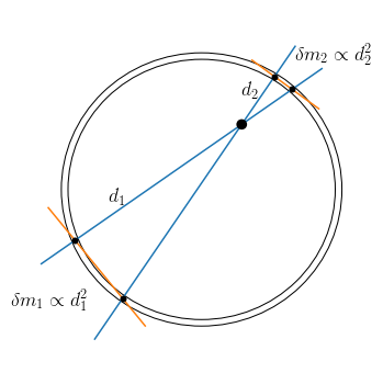
For a narrow cone, the surface of the intersection between the cone and the shell is approximately that of the cone and a plane; such an intersection is a conical section and in this case in particular, an ellipse. The major and minor axis are the segment of the orange line between the two dots in the figure above (major or minor depending on the projection). For small opening angles, the ratio of the lengths of these axes is equal to the ratio of the distances between the center of the cone and the intersections: \(d_1/d_2\) in the figure above. Therefore, the ratio of the areas of the ellipses is \(d_1^2/d_2^2\) and, because the shell has uniform density and thickness, the ratio of the masses is the same. Because of the \(1/r^2\) dependence of the gravitational force, the gravitational forces from the two intersections are then equal in magnitude and opposite in sign and they therefore cancel. This holds for any narrow cone centered on any point within the shell and, therefore, there is no net force from the shell on any interior point.
The first theorem implies that for a spherical mass distribution, mass outside of the current radius of a body has no influence on the motion of that body (at the present time). In particular, for a body on a circular orbit, the mass outside of this circle has no effect on the entire orbit. We will see in Chapter 8 that this is not the case for flattened mass distributions (the geometric proof of Newton’s first theorem immediately makes it clear why it does not hold for flattened distributions).
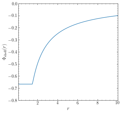
Newton’s second shell theorem implies that the gravitational potential outside of a shell of radius \(R\) is
The first theorem together with the requirement that the potential is continuous at \(R\) then implies that the gravitational potential within a shell of radius \(R\) is equal to
An example of the potential of a shell at \(r=1.5\) is:
[8]:
from galpy.potential import SphericalShellPotential
from galpy.util import plot as galpy_plot
sp= SphericalShellPotential(a=1.5)
rs= numpy.linspace(0.1,10.,101)
galpy_plot.plot(rs,[sp(r,0.) for r in rs],
                yrange=[-.8,0.],
                xlabel=r'$r$',ylabel=r'$\Phi_{\mathrm{shell}}(r)$');
To obtain the gravitational potential at radius \(r\) due to a spherical mass distribution \(\rho(r')\), we can therefore sum the contributions from all shells with mass \(\mathrm{d}M(r') = 4\pi G\rho(r')r'^2\mathrm{d}r'\) inside and outside of \(r\) as follows
One can show that this satisfies the Poisson equation using the Laplacian in spherical coordinates (Equation A.12). Thus, for spherical mass distributions, we can compute the potential \(\Phi\) using a simple quadrature for any mass distribution \(\rho(r)\).
As an example, we discretize the mass distribution of a Plummer profile (see below) into a small number of shells where each shell contains the mass between the radius of the shell just inside it and the shell’s radius (and the innermost shell contains all mass up to its radius). We can do this with the following function, which creates a galpy potential that is a set of discrete shells defined in this way for any spherical potential:
[9]:
from scipy import integrate
def discretize_potential_into_shells(pot,rmin,rmax,dr):
    rs= numpy.arange(rmin,rmax+dr,dr)
    dM= numpy.empty_like(rs)
    dM[0]= 4.*numpy.pi*integrate.quad(lambda r: r**2*pot.dens(r,0.),
                                      0.,rs[0])[0]
    for ii in range(1,len(rs)):
        dM[ii]= 4.*numpy.pi*integrate.quad(lambda r: r**2*pot.dens(r,0.),
                                           rs[ii-1],rs[ii])[0]
    return [SphericalShellPotential(amp=dm,a=r) for (dm,r) in zip(dM,rs)]
Applying this for a Plummer profile with scale parameter \(b=1.5\), using shells spaced \(\Delta r = 1\) apart out to \(r = 3\times b\) gives:
[10]:
from galpy.potential import PlummerPotential, evaluatePotentials
pp= PlummerPotential(amp=1.,b=1.5)
rmin, rmax, dr= 0.5,4.5,1.
discrete_pp= discretize_potential_into_shells(pp,rmin,rmax,dr)
line_approx= galpy_plot.plot(rs,[evaluatePotentials(discrete_pp,r,0.)
                                 for r in rs],
                             yrange=[-.75,0.],
                             xlabel=r'$r$',ylabel=r'$\Phi(r)$',
                             label=r'$\mathrm{Shell\ approximation}$'\
                              +'\n'+r'$r_\mathrm{max}=3b, \Delta r=1$')
line_plummer= galpy_plot.plot(rs,pp(rs,0.),overplot=True,zorder=0,
                              label=r'$\mathrm{Plummer}$')
legend(handles=[line_approx[0],line_plummer[0]],
       fontsize=18.,loc='lower right',frameon=False);
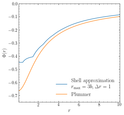
The orange curve shows the actual potential for a Plummer profile (given in Section 3.4.3 below). We see the discreteness of the approximation clearly at \(r \lesssim 2b\), but at larger \(r\) the approximation becomes largely smooth because most of the mass is within a few times \(b\) for a Plummer profile. We also notice that the approximation, while smooth, remains too high at large \(r\). Decreasing the spacing of the shells improves the agreement at small \(r\):
[11]:
rmin, rmax, dr= 0.5,4.5,0.1
discrete_pp= discretize_potential_into_shells(pp,rmin,rmax,dr)
line_approx= galpy_plot.plot(rs,[evaluatePotentials(discrete_pp,r,0.)
                                 for r in rs],
                             yrange=[-.75,0.],
                             xlabel=r'$r$',ylabel=r'$\Phi(r)$',
                             label=r'$\mathrm{Shell\ approximation}$'\
                              +'\n'+r'$r_\mathrm{max}=3b, \Delta r=0.1$')
line_plummer= galpy_plot.plot(rs,pp(rs,0.),overplot=True,zorder=0,
                              label=r'$\mathrm{Plummer}$')
legend(handles=[line_approx[0],line_plummer[0]],
       fontsize=18.,loc='lower right',frameon=False);
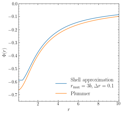
But there is still an overall offset between the shells and the true potential. This is because we are ignoring the mass at \(r > 3b\), thus clearly showing that the potential—unlike the force—at \(r\) depends on the mass profile outside of \(r\). We therefore edit our shell-discretization function to let the final shell contain all mass out to infinity:
[12]:
def discretize_potential_into_shells(pot,rmin,rmax,dr):
    rs= numpy.arange(rmin,rmax+dr,dr)
    dM= numpy.empty_like(rs)
    dM[0]= 4.*numpy.pi*integrate.quad(lambda r: r**2*pot.dens(r,0.),
                                      0.,rs[0])[0]
    for ii in range(1,len(rs)-1):
        dM[ii]= 4.*numpy.pi*integrate.quad(lambda r: r**2*pot.dens(r,0.),
                                           rs[ii-1],rs[ii])[0]
    dM[-1]= 4.*numpy.pi*integrate.quad(lambda r: r**2*pot.dens(r,0.),
                                       rs[ii],numpy.inf)[0]
    return [SphericalShellPotential(amp=dm,a=r) for (dm,r) in zip(dM,rs)]
Using this function and using shells out to \(r = 5b\) then gives:
[13]:
rmin, rmax, dr= 0.5,7.5,0.1
discrete_pp= discretize_potential_into_shells(pp,rmin,rmax,dr)
line_approx= galpy_plot.plot(rs,[evaluatePotentials(discrete_pp,r,0.)
                                 for r in rs],
                             yrange=[-.75,0.],
                             xlabel=r'$r$',ylabel=r'$\Phi(r)$',
                             label=r'$\mathrm{Shell\ approximation}$'\
                              +'\n'+r'$r_\mathrm{max}=5b, \Delta r=0.1$')
line_plummer= galpy_plot.plot(rs,pp(rs,0.),overplot=True,zorder=0,
                              label=r'$\mathrm{Plummer}$')
legend(handles=[line_approx[0],line_plummer[0]],
       fontsize=18.,loc='lower right',frameon=False);
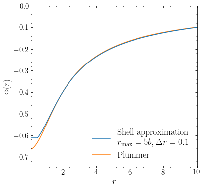
Now we have almost perfect agreement for all but the innermost part of the potential well.
The only non-zero component of the gravitational field is the radial component \(g_r\), which is given by
where \(M(<r)\) is the mass contained within radius \(r\). This can be derived directly from Newton’s theorems or by taking the derivative from Equation (\(\ref{eq-spherpot}\)) for the potential. Because \(g_r(r) = -\partial \Phi(r) / \partial r\), this gives an alternate relation between the enclosed mass and the potential
or
You can show that Equation \(\eqref{eq-spherpot-encmassdens}\) is equal to Equation \(\eqref{eq-spherpot}\) by changing the order of the integration (carefully). These forms can make the calculation of the potential easier if the enclosed mass has a known, simple form.
3.3. Circular velocity and dynamical time
Next we introduce some of the most basic properties of mass distributions, those of circular velocity and dynamical time. We define these here based on the properties of circular orbits and they therefore require equations for the motion of a body under the influence of gravity. We discuss these equations in far more detail in Chapters 4.1 and 5. All we need for the purposes of this discussion is that for a circular orbit, the centripetal acceleration \(a_r=-v^2/r\) is balanced by the gravitational field. Thus, for a spherical mass distribution using Equation \(\eqref{eq-sphere-gr}\) we have
or
This velocity is the circular velocity \(v_c\) at radius \(r\). This equation directly shows that the circular velocity at radius \(r\) is a direct measure of the total mass contained within that radius and measuring the circular velocity as a function of \(r\) therefore directly measures the mass distribution of a spherical distribution. We will see in Chapter 8 that even for very flattened systems, like disk galaxies, the circular velocity is of a similar magnitude as if the flattened mass were distributed spherically. So the circular velocity measures the mass distribution well even for such systems. For reference, the Sun orbits the center of the Milky Way at a distance of \(R_0 \approx 8\,\mathrm{kpc}\) where the circular velocity is \(v_c \approx 220\,\mathrm{km\,s}^{-1}\). Assuming that the mass within the solar orbit is distributed spherically (a rather poor assumption), the values of \(r = 8\,\mathrm{kpc}\) and \(v_c = 220\,\mathrm{km\,s}^{-1}\) mentioned above give an enclosed mass of
By comparing to the mass within 8 kpc in a sophisticated mass model for the Milky Way that is shown in Chapter 2.2.3, you can see that this estimate is actually quite accurate!
We can immediately use the relation between the circular velocity and the mass distribution to understand how we know of the presence of dark matter in galaxies (a preview of what we will discuss in detail in Chapter 9). Interstellar gas orbits the centers of galaxies on approximately circular orbits and the velocity of the gas can be measured through Doppler shifts of radio emission lines (like the 21 cm line). This allowed researchers in the 1970s and 1980s to measure the rotation curves—the circular velocity \(v_c(r)\) as a function of \(r\)—at distances \(r\) where few stars and little gas are observed to be present. What they found was that \(v_c\) is almost constant with \(r\). Re-arranging Equation (\(\ref{eq-vcirc}\)) above shows that this implies that the mass distribution behaves as
the cumulative mass increases linearly with \(r\). Given that little stellar or gaseous material is observed, this implied the existence of a large amount of dark matter in galaxies.
We can define the crossing time or dynamical time as the time necessary to cross the galaxy, \(t_\mathrm{dyn} \approx R /v\). More formally, we may define the dynamical time at \(r\) as the period of a circular orbit at \(r\), the time it takes to orbit the galaxy (or other stellar system) once
Note that this is not the only possible definition, but all other definitions would involve \(r/v_c\), perhaps with a different pre-factor (see the discussion of the homogeneous sphere below for more justification for this). Using the relation between \(v_c\) and \(M(<r)\) we can express the dynamical time in terms of the average density
where \(\bar{\rho}\) is the average density within radius \(r\): \(\bar{\rho} = M(<r)/(4\pi r^3/3)\). Thus we have that \(t_\mathrm{dyn} \propto (G\bar{\rho})^{-1/2}\). This formula provides a simple and general way to estimate the dynamical time of any mass distribution, spherical or otherwise. Systems of high average density (such as the centers of galaxies or the centers of globular clusters) have short dynamical times, while low average density regions (such as the outskirts of the halos of galaxies) have long dynamical time scales.
For galaxies, the dynamical times are typically hundreds of Myr to Gyr. For example, using the distance and velocity of the Sun within the Milky Way quoted above, we get that the dynamical time is
Because galactic rotation curves are close to flat, the dynamical time scales approximately as the distance to the center and, thus, it drops to tens of Myr in the inner kpc and increases to 1 Gyr at \(r \gtrsim 50\) kpc. Galaxies are about 10 Gyr old today, which depending on where you are in the galaxy corresponds to a few dynamical times (in the outskirts) to a few thousand dynamical times (in the innermost regions, with the solar neighborhood being about 40 dynamical times old. Compared to, for example, the \(\approx 4.6\times 10^9\) times that the Earth has gone around the Sun, galaxies are dynamically young.
3.4. Examples of spherical potentials
Let’s now consider some example spherical potentials that illustrate the concepts above. This is by no means an exhaustive list of spherical potentials, but they are main ones that we will use in the rest of this book and some of the main ones that often come up in research. More examples are discussed in the exercises.
3.4.1. Point-mass potential
The most basic spherical potential is that of a point mass. As we demonstrated in Section 3.1 above, the potential is
for a point mass \(M\). Because of Newton’s second shell theorem, this is also the potential outside the boundary for any spherical mass distribution with a finite extent. Any potential with a total finite mass should also approach the point-mass potential as \(r \rightarrow \infty\).
The circular velocity is given by
The point-mass potential of the Sun is the dominant gravitational potential that sets planetary trajectories in the solar system (perturbations from other planets are very small). Because Equation \(\eqref{eq-vc-kepler}\) is equivalent to Kepler’s third law, first proposed by Kepler, the point-mass potential and orbits within it are often referred to as Keplerian. For example, a disk of mass \(m \ll M\) orbiting a point mass is Keplerian and is in Keplerian rotation. Keplerian orbits have special properties that we discuss in more detail in the next chapters.
In galactic dynamics, point-mass potentials are typically only used to represent the gravitational field from (supermassive) black holes or as an approximation. Point-mass potentials are not typically used in \(N\)-body simulations of galaxies as we will discuss in Chapter 19: the gravitational potential of individual particles in \(N\)-body simulations is smoothed to, for example, a Plummer potential (see below) to avoid the force divergence for (unphysical) close encounters; these encounters are unphysical because galaxies are collisionless. \(N\)-body simulations of stellar clusters do use the point-mass potentials for all of their constituent stars.
3.4.2. The homogeneous sphere
The potential of a homogeneous density sphere, \(\rho(r) = \rho_0 =\) constant for all \(r < R\) and zero at \(r \geq R\), can be calculated using \(\eqref{eq-spherpot}\); the result is
At \(r<R\), this quadratic potential is that of a harmonic oscillator; we only consider \(r < R\) in the following, because at \(r \geq R\) the behavior is the same as that of the point-mass potential above due to Newton’s second shell theorem. The circular velocity is
and the dynamical time using the definition from \(\eqref{eq-tdyn}\) is therefore
The dynamical time in Equation \(\eqref{eq-tdyn-homogeneous}\) is the same as that we derived in Equation \(\eqref{eq-tdyn-dens}\) when substituting \(\rho_0\) for the average density. In a homogeneous sphere, the dynamical time is constant with \(r\). If instead of considering a body on a circular orbit, we look at a body moving perfectly radially, it’s equation of motion according to Newton’s second law is
which is the equation of motion of a simple harmonic oscillator with frequency \(\omega = \sqrt{4\pi\,G\,\rho_0/3}\). The period of this radial oscillation is
which is again constant. This result provides further justification for the definition of the dynamical time in \(\eqref{eq-tdyn}\): no matter whether a body is on a circular orbit or a purely radial orbit, the period of the orbit is \(\approx t_\mathrm{dyn}\).
Because \(v_c(r) \propto r\) for a homogeneous sphere, a disk of bodies rotates with an angular rotation rate of \(\Omega(r) = v_c(r)/r =\) constant. Because the rotation rate is constant, such a disk rotates as a solid body and this setup is referred to as solid-body rotation.
3.4.3. Plummer sphere
Next we will look at a few generalizations of the Kepler point-mass potential above that often crop up in the study of galaxies. One of the most important of these is the Plummer model (Plummer 1911), which smooths the Kepler potential for a mass \(M\) by replacing the radius \(r\) in the denominator of Equation \(\eqref{eq-pot-kepler}\) by \(\sqrt{r^2+b^2}\) where \(b\) is a constant, the Plummer scale length,
This potential approaches a Kepler potential as \(b \rightarrow 0\), or, put in a way that is more practically useful, \(r \gg b\). The Plummer potential was originally introduced to represent globular clusters, but is no longer a preferred model for these systems. It remains highly useful because it has many convenient analytical properties and provides a crude model for, e.g., dark matter halos that is easy to work with; it is also used to represent the stellar density in small dwarf galaxies. Finally, it also provides a simple kernel used to smooth the gravitational field of point particles in \(N\)-body simulations.
It is straightforward to derive the circular velocity from Equation \(\eqref{eq-pot-plummer}\). The density profile using the Poisson equation is
3.4.4. Isochrone potential
Similar to the Plummer sphere, the isochrone potential is obtained by smoothing the potential of a point mass (Henon 1959). For the isochrone potential, this is done by replacing \(r\rightarrow b+\sqrt{r^2+b^2}\) in the denominator of the gravitational potential (see Equation \([\ref{eq-pot-kepler}]\)), where \(b\) is again a constant
Similar to the Plummer sphere, this potential approaches a Kepler potential when \(b \rightarrow 0\), or when \(r \gg b\). We can determine how fast the isochrone model approaches the Kepler potential by expanding the potential around \(b/r\) for \(r \gg b\)
Because the first term is the potential of a point mass, which has zero density at \(r \neq 0\), the density at large radii is given by that corresponding to the second term, \(\Phi(r) \propto r^{-2}\). From the Poisson equation, we know that the density is a second derivative of the potential, and must therefore tend to \(\rho_{r\gg b}(r) \propto r^{-4}\). This \(1/r^4\) behavior is also that of a popular model for dark-matter halos, the Hernquist model. We will discuss power-law potentials and the Hernquist model in more detail below.
When \(r/b \rightarrow 0\), we can expand the potential around \(r/b\)
Up to an irrelevant constant, this is the potential of a homogeneous sphere with density \(\rho_0 = 3\,M/(16\pi\,b^3)\). This immediately tells us that the central density of the isochrone mass distribution is this \(\rho_0\).
Thus, the isochrone potential smoothly interpolates between the potential of a point mass and that of a homogenous density distribution, essentially the two extremes of the types of densities seen in stellar systems.
The circular velocity of the isochrone potential is given by
where \(a = \sqrt{r^2+b^2}\).
It is clear that the isochrone model can represent a wide range of potentials. Because it interpolates between the two extremes of density distributions, over a narrow radial range it can essentially represent all spherical potentials. But the main reason for the importance of the isochrone potential is that it is the most realistic model for galaxies in which all of the orbits can be solved analytically (Saha 1991). That is, just like for the Kepler potential, we can work out the full orbit of a body in terms of elementary functions, without requiring any numerical quadrature or numerically solving the differential equation of motion. Naturally, the analytic solution is more complicated than that for a Kepler potential, but not so much more so (like for Keplerian orbits, we only need to solve a single transcendental equation, a generalization of Kepler’s equation). That all of the orbits are analytic is extremely useful in many settings in galactic dynamics.
Let’s compare the rotation curves of the spherical potentials that we have discussed so far by plotting them with galpy. We normalize the point-mass, Plummer, and isochrone potentials such that they all have \(G\,M = 1\), and the homogeneous sphere such that \(v_c = 1\) for \(r = 1\). We set the scale \(b\) of the isochrone and Plummer potentials to \(b=1\) and we set the size of the homogeneous sphere to be larger than the radial range that we consider such that its
density is constant everywhere that we consider here.
[14]:
from galpy import potential
figsize(10,6)
# Define each potential
kp= potential.KeplerPotential(amp=1.)
hp= potential.HomogeneousSpherePotential(normalize=1.,R=20.)
pp= potential.PlummerPotential(amp=1.,b=1.)
ip= potential.IsochronePotential(amp=1.,b=1.)
# Plot the rotation curve for each
line_kepler= potential.plotRotcurve(kp,Rrange=[0.,10.],\
                label=r'$\mathrm{Point\ mass}$',yrange=[0.,1.5],
                xlabel=r'$r$',ylabel=r'$v_c(r)$')
line_homog= potential.plotRotcurve(hp,Rrange=[0.,10.],\
                label=r'$\mathrm{Homogeneous\ sphere}$',overplot=True)
line_plummer= potential.plotRotcurve(pp,Rrange=[0.,10.],\
                label=r'$\mathrm{Plummer}\,(b=1)$',overplot=True)
line_isochrone= potential.plotRotcurve(ip,Rrange=[0.,10.],\
                label=r'$\mathrm{Isochrone}\,(b=1)$',overplot=True)
legend(handles=[line_kepler[0],line_homog[0],
                line_plummer[0],line_isochrone[0]],
       fontsize=18.,loc='upper right',frameon=False);
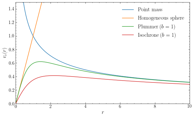
We see the expected behavior in these curves: the point-mass \(v_c(r)\) drops as \(r^{-1/2}\), while the other potentials all have \(v_c(r) \propto r\) at \(r \ll b\) (and everywhere for the homogeneous sphere, which quickly runs out of the shown range in \(v_c\)), because they all have an approximate constant-density core. At \(r > b\) the Plummer and isochrone potentials approach the Keplerian curve, because they all have the same total mass. The Plummer potential approaches the Keplerian curve quicker than the isochrone potential for the same \(b\).
3.4.5. Power-law models
An important class of models are those in which the density is a power-law of radius
where \(\rho_0\) is the density at \(r=r_0\). The enclosed mass of this density profile is
which is finite at \(r=\infty\) only when \(\alpha > 3\). Using Equation \(\eqref{eq-spherpot-encmass}\), we find that the potential is
and
The circular velocity is given by
For \(\alpha = 2\) the circular velocity is constant with \(v_c =\sqrt{4\pi\,G\,\rho_0\,r_0^2}\) and we can write the gravitational potential in Equation \(\eqref{eq-pot-powlaw-log}\) in terms of \(v_c\)
This is an important potential that is, for obvious reasons, often referred to as the logarithmic potential. Because it gives rise to a constant circular velocity—a flat rotation curve—it is a very simple and often-used model for the potential of galaxies with a flat rotation curve. When we study self-consistent dynamical equilibrium states in Chapter 6, we will see that for the logarithmic potential the velocity dispersion is constant with \(r\) and it is therefore also often referred to as the singular isothermal sphere, with the “singular” modifier due to the \(1/r^2\) density divergence as \(r\rightarrow 0\).
3.4.6. Two-power density models
A final important class of spherical potentials for galaxies are those that are described by a different power law in their inner and outer parts, with a smooth transition region between the two. A popular set of models with this property is that with the following density law
In the small and large \(r\) limit, these models behave as power law models
The inner slope is therefore \(\alpha\) and the outer slope is \(\beta\), with the transition occurring around \(r \approx a\), where \(a\) is known as the scale radius. The second parameter of these profiles, \(\rho_0\), gives a typical density, because it is the density at the scale radius up to a numerical factor that depends on \(\alpha\) and \(\beta\). For \(\beta=4\), these models have relatively simple properties and they are known as \(\gamma\) models (where \(\gamma\) is what we call \(\alpha\) above); Dehnen (1993) and Tremaine et al. (1994) provide more information on this set of models. We will only consider two popular instances of two-power density models: the Hernquist model (Hernquist 1990), which has \(\alpha = 1, \beta =4\), and the Navarro-Frenk-White (NFW; Navarro et al. 1997) model, with \(\alpha = 1, \beta = 3\). The enclosed mass is given by
Using Equation \(\eqref{eq-spherpot-encmass}\), this gives the gravitational potential
The total mass of an NFW potential does not converge as we increase \(r\), but Equation \(\eqref{eq-massenc-hernnfw}\) demonstrates that the total mass of a Hernquist potential is \(M = 2\pi\,\rho_0\,a^3\). The Hernquist potential written in terms of this mass \(M\) is
The Hernquist potential is therefore also a simple smoothing of the Kepler point-mass potential (like the Plummer model), in this case by replacing \(r \rightarrow r+a\). As for the Plummer model, this often means that calculations involving a Hernquist potential can be analytically simplified. Another member of this family (and of the \(\gamma\) models) is that with \(\alpha=2\) and \(\beta=4\), the Jaffe profile, which is often used to represent very cuspy profiles because of its convenient analytical properties (Jaffe 1983).
The NFW profile is found to describe the density profile of dark matter halos well in cosmological simulations (Navarro et al. 1996) and remains highly important for this reason. Hernquist profiles have somewhat more tractable properties and are also a popular model for dark matter halos and for elliptical galaxies and galactic bulges, because they can approximately represent the \(R^{1/4}\) de Vaucouleurs surface-brightness profile of ellipticals and bulges (see Chapter 13.1). The outskirts of dark-matter halos at the present time have not yet fully formed and it has also been argued that the long-term state of dark-matter halos more closely resembles a Hernquist profile than an NFW profile (Busha et al. 2005).
Let’s compare the rotation curves of Hernquist and NFW potentials with the same scale radius \(a\). First, we compare the rotation curves for the case where both potentials correspond to the same enclosed mass at \(r= 12\,a\) (this is approximately the virial radius for Milky-Way-mass dark-matter halos). We do this by computing the enclosed mass using galpy’s .mass function for each potential set up with an amplitude of unity and then setting the new amplitude such that both
potentials have the same mass:
[15]:
from galpy import potential
from galpy.util import plot as galpy_plot
figsize(10,6)
# Define each potential, equal mass at 12 scale radii
hp_4scale= potential.HernquistPotential(amp=1.,a=1.)
hp= potential.HernquistPotential(amp=10./hp_4scale.mass(12.),a=1.)
nfp_4scale= potential.NFWPotential(amp=1.,a=1.)
nfp= potential.NFWPotential(amp=10./nfp_4scale.mass(12.),a=1.)
# Plot the rotation curve for each
line_hernquist= potential.plotRotcurve(hp,Rrange=[0.,15.],\
                label=r'$\mathrm{Hernquist}$',yrange=[0.,2.5],
                xlabel=r'$r/a$',ylabel=r'$v_c(r/a)$')
line_nfw= potential.plotRotcurve(nfp,Rrange=[0.,15.],\
                label=r'$\mathrm{NFW}$',overplot=True)
legend(handles=[line_hernquist[0],line_nfw[0]],
       fontsize=18.,loc='upper right',frameon=False)
galpy_plot.text(r'$\mathrm{Equal\ mass\ at}\ R=12\,a$',
                top_left=True,size=18.)
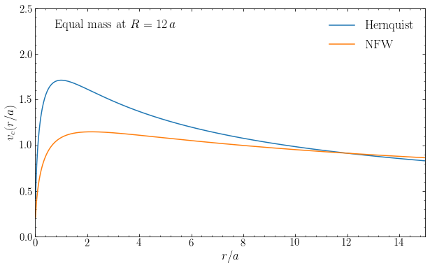
Because both potentials are defined to have the same mass at \(r=12\,a\), the circular velocity at these radii is the same. We see that the rotation curve of the Hernquist potential reaches a much higher maximum value than the NFW potential with the same mass, because the Hernquist sphere’s mass is much more concentrated than that of the NFW sphere. At \(r > 12\,a\), the Hernquist \(v_c(r)\) declines more steeply with radius than the NFW \(v_c(r)\), because of the \(r^{-4}\) behavior of the density at \(r \gg a\) for the Hernquist profile versus the \(r^{-3}\) behavior for the NFW density.
Next, let’s compare the rotation curves if we normalize the Hernquist and NFW potentials such that they have the same inner density profile \(\rho(r) \propto \rho_0\,r^{-1}\) at \(r \ll a\):
[16]:
figsize(10,6)
# Define each potential, equal inner profile
hp= potential.HernquistPotential(amp=20.,a=1.)
nfp= potential.NFWPotential(amp=20.,a=1.)
# Plot the rotation curve for each
line_hernquist= potential.plotRotcurve(hp,Rrange=[0.,15.],\
                label=r'$\mathrm{Hernquist}$',yrange=[0.,2.5],
                xlabel=r'$r/a$',ylabel=r'$v_c(r/a)$')
line_nfw= potential.plotRotcurve(nfp,Rrange=[0.,15.],\
                label=r'$\mathrm{NFW}$',overplot=True)
legend(handles=[line_hernquist[0],line_nfw[0]],
       fontsize=18.,loc='upper right',frameon=False)
galpy_plot.text(r'$\mathrm{Equal\ inner\ density\ profile}$',
               top_left=True,size=18.)
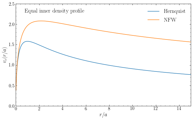
The inner rotation curves are now the same, because the enclosed mass profile is the same at \(r \ll a\), but because the density of the NFW profile is shallower than that of the Hernquist profile, the NFW rotation curve reaches a significantly higher value than that of the Hernquist profile.
NFW models for dark-matter halso are in widespread use and there are various other ways to parametrize these beside the \((\rho_0,a)\) parameterization used in Equation \eqref{eq-twopower-dens} (which is, in fact, not commonly used). The most important of these is the parameterization using the virial mass and concentration. As we discussed above, NFW models do not have a finite mass, so any mass parameter has to be defined within a specified radius. The virial mass is the mass within the virial radius. We will discuss the gravitational collapse and virialization of dark-matter halos in detail in Chapter 18.2.2, but one thing we will derive there is that after formation, the virialized part of dark-matter halos has a radial extent—the virial radius—within which the mean density is a constant factor \(\Delta_v\) times the Universe’s critical density (the density for which the Universe is spatially flat, \(\rho_\mathrm{crit} = 3 H^2/[8\pi G]\), with \(H\) the Hubble parameter; see Chapter 18). This factor is often set to 200, although technically this factor depends on a halo’s formation redshift and it is only \(\approx 200\) at \(z \gtrsim 2\). To relate the virial radius to the \((\rho_0,a)\) parameterization used in Equation \eqref{eq-twopower-dens}, we first compute the mean density within a given radius for the NFW profile using Equation \eqref{eq-massenc-hernnfw}
At the virial radius \(r_\mathrm{vir}\), this mean density should equal \(\Delta_v \rho_\mathrm{crit}\)
where \(c\) is the concentration, \(c = r_\mathrm{vir}/a\), the second parameter used in the (virial mass,concentration) parameterization. The expression in parentheses is often abbreviated as \(f(c)\)
Because of the definition of the virial radius, we have the following relation between virial mass \(M_\mathrm{vir}\) and virial radius
Thus, given a pair \((M_\mathrm{vir},c)\) and a value of \(\Delta_v\), we can set the amplitude parameter \(\rho_0\) using
and \(\rho_0\) therefore only depends on the concentration and is independent of the virial mass. Similarly, we obtain \(a = r_\mathrm{vir}/c\) or
Conversely, to determine \(M_\mathrm{vir}\) and \(c\) for a given \(\rho_0\) and \(a\), we need to numerically solve Equation \eqref{eq-meandens-nfw-atrvir} for \(c\), compute \(r_\mathrm{vir} = a\,c\), and obtain \(M_\mathrm{vir}\) from Equation \eqref{eq-nfw-mvir-rvir}. In terms of \((M_\mathrm{vir},c,r_\mathrm{vir})\), the enclosed mass profile is given by
Another popular way of parameterizing NFW halos is by the maximum of the circular-velocity curve, \(v_\mathrm{max}\), and the radius \(r_\mathrm{max}\) at which this maximum occurs. This is an especially useful parameterization to use when analyzing \(N\)-body simulations of dark-matter halos, because these quantities are easy to measure from the simulation. To relate this to the other parameterizations, we first derive the rotation curve of an NFW profile by combining Equations \eqref{eq-vcirc} and \eqref{eq-nfw-encmass-invirial}
Only the second fraction in the second expression depends on \(r\) and to find the radius of the maximum, we only need to consider this factor; we find the maximum by setting the derivative of this expression to zero, using \(x \equiv r/a\) as the variable
This function looks like
[28]:
xs= numpy.linspace(0.,12.,101)
plot(xs,-numpy.log(1+xs)/xs+(2.*xs+1)/(1.+xs)**2.)
xlabel(r'$x$')
ylabel(r'$\mathrm{d} [f(x)/x] / \mathrm{d} x)$');
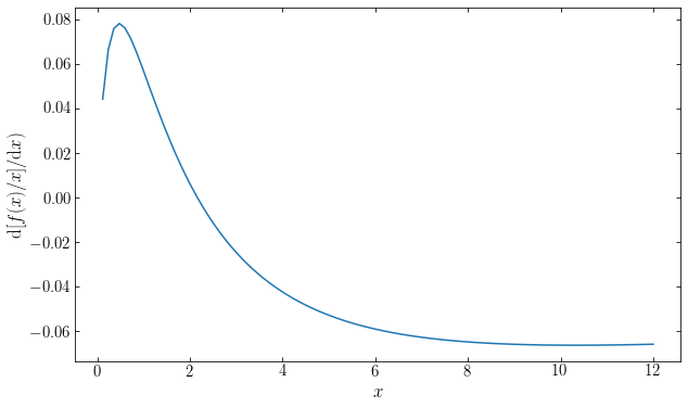
and we can find the exact location of \(x_\mathrm{max}\) by finding the root of this function:
[29]:
from scipy import optimize
print("The NFW rotation curve peaks at r/a = {:.16f}".format(
    optimize.brentq(lambda x: -numpy.log(1+x)/x+(2.*x+1)/(1.+x)**2.,0.1,10)))
The NFW rotation curve peaks at r/a = 2.1625815870646115
Thus, we have that
or using Equation \eqref{eq-nfw-a-frommvirc}
Note that the relation between \(r_\mathrm{max}\) and \(a\) does not depend on the second parameter of the NFW profile (\(\rho_0\), \(M_\mathrm{vir}\), or \(v_\mathrm{max}\)). To get \(v_\mathrm{max}\), we then substitute \(r_\mathrm{max}\) into Equation \eqref{eq-nfw-vc2} and we get
where \(0.21621659550187314= f(2.1625815870646115)/2.1625815870646115\), or in terms of \((\rho_0,a)\)
Because \(\sqrt{G M_\mathrm{vir}/ r_\mathrm{vir}}\) is the circular velocity \(v_{c,\mathrm{vir}}\) at the virial radius, we can also write this as
where 2.6 is a typical value for \(\sqrt{c/f(c)}\) (which varies by only \(\approx\pm 10\,\%\) for relevant concentrations).
Large numerical simulations of the formation of dark-matter halos in Universes with similar cosmological parameters as our own have shown that the formed dark-matter halos populate only a narrow sequence in the space of \((M_\mathrm{vir},c)\) following a relation between \(M_\mathrm{vir}\) and \(c\) (Navarro et al. 1996, Navarro et al. 1997). Such relations are known as concentration–mass relations and they are updated every few years whenever a new set of best-fit cosmological parameters are determined, but a representative relation is the redshift zero relation of Dutton & Macciò (2014)
where \(\Delta_v = 200\) and the authors use a Hubble constant of \(H_0 = 100\,h\,\mathrm{km\,s}^{-1}\,\mathrm{Mpc}^{-1} = 67.1\,\mathrm{km\,s}^{-1}\,\mathrm{Mpc}^{-1}\) following Planck Collaboration et al. (2014). The following figure shows the relation between the two parameters in all three parameterizations of the NFW profile for this concentration–mass relation from the scale of the smallest dwarf galaxies to that of large clusters of galaxies:
[140]:
from galpy.potential import NFWPotential
from matplotlib.ticker import FuncFormatter
from matplotlib.cm import autumn, winter
def dutton14_conc(m200):
    return 10.**(0.905-0.101*numpy.log10(m200*0.671/10.**12/u.Msun))
m200s= numpy.geomspace(1e7,1e15,101)*u.Msun
cs= numpy.linspace(2.,28.,101)
const_cs= numpy.arange(5,30,5)
const_m200s= numpy.geomspace(1e8,1e14,7)
const_c_cmap= autumn
const_m200_cmap= winter
figsize(10,5)
subplot(1,3,1)
galpy_plot.plot(m200s.to_value(u.Msun),dutton14_conc(m200s),
                semilogx=True,gcf=True,color='k',lw=3.,
                xrange=[3e6,3e15],
                yrange=[0.,30],
                xlabel=r'$M_\mathrm{vir} / M_\odot$',
                ylabel=r'$c$')
for const_c in const_cs:
    plot(m200s.to_value(u.Msun),
         const_c*numpy.ones_like(m200s.to_value(u.Msun)),
         color=const_c_cmap((const_c-5.)/20.),lw=1.5,zorder=0)
for const_m200 in const_m200s:
    plot(const_m200*ones_like(cs),
         cs,
         color=const_m200_cmap((numpy.log10(const_m200)-8.)/6),
         lw=1.5,zorder=0)
subplot(1,3,2)
# Set up NFWPotentials for each (mvir,conc)
nps= [NFWPotential(mvir=m200.to_value(1e12*u.Msun),
                   conc=dutton14_conc(m200).to_value(u.dimensionless_unscaled),
                   H=67.1,overdens=200.,wrtcrit=True,
                   ro=8.,vo=220.)
      for m200 in m200s]
# rho0 = 4 rho(a) from definition
galpy_plot.plot([4.*np.dens(np.a,0.).to_value(u.Msun/u.pc**3) for np in nps],
                [np.a*np._ro for np in nps],
                loglog=True,gcf=True,color='k',lw=3.,
                xrange=[3e-4,9e-2],
                yrange=[0.08,900],
                xlabel=r'$\rho_0\,(M_\odot\,\mathrm{pc}^{-3})$',
                ylabel=r'$a\,(\mathrm{kpc})$')
# Also for const_cs
all_const_cs_nps= []
for const_c in const_cs:
    all_const_cs_nps.append([NFWPotential(mvir=m200.to_value(1e12*u.Msun),
                                          conc=const_c,
                                          H=67.1,overdens=200.,wrtcrit=True,
                                          ro=8.,vo=220.)
                             for m200 in m200s])
    plot([4.*np.dens(np.a,0.).to_value(u.Msun/u.pc**3) for np in all_const_cs_nps[-1]],
         [np.a*np._ro for np in all_const_cs_nps[-1]],
         color=const_c_cmap((const_c-5.)/20.),lw=1.5,zorder=0)
# Also for const_m200s
all_const_m200s_nps= []
for const_m200 in const_m200s:
    all_const_m200s_nps.append([NFWPotential(mvir=const_m200/1e12,
                                             conc=c,
                                             H=67.1,overdens=200.,wrtcrit=True,
                                             ro=8.,vo=220.)
                                for c in cs])
    plot([4.*np.dens(np.a,0.).to_value(u.Msun/u.pc**3) for np in all_const_m200s_nps[-1]],
         [np.a*np._ro for np in all_const_m200s_nps[-1]],
         color=const_m200_cmap((numpy.log10(const_m200)-8.)/6),
         lw=1.5,zorder=0)
gca().xaxis.set_major_formatter(FuncFormatter(
                lambda y,pos: (r'${{:.{:1d}f}}$'.format(int(\
                    numpy.maximum(-numpy.log10(y),0)))).format(y)))
gca().yaxis.set_major_formatter(FuncFormatter(
                lambda y,pos: (r'${{:.{:1d}f}}$'.format(int(\
                    numpy.maximum(-numpy.log10(y),0)))).format(y)))
subplot(1,3,3)
galpy_plot.plot([np.rmax().to_value(u.kpc) for np in nps],
                [np.vmax().to_value(u.km/u.s) for np in nps],
                loglog=True,gcf=True,color='k',lw=3.,
                xrange=[0.15,3000.],
                yrange=[0.5,3000.],
                xlabel=r'$r_\mathrm{max}\,(\mathrm{kpc})$',
                ylabel=r'$v_\mathrm{max}\,(\mathrm{km\,s}^{-1})$')
# Also for const_cs
for const_c,const_cs_nps in zip(const_cs,all_const_cs_nps):
    plot([np.rmax().to_value(u.kpc) for np in const_cs_nps],
         [np.vmax().to_value(u.km/u.s) for np in const_cs_nps],
          color=const_c_cmap((const_c-5.)/20.),lw=1.5,zorder=0)
# Also for const_m200s
for const_m200,const_m200s_nps in zip(const_m200s,all_const_m200s_nps):
    plot([np.rmax().to_value(u.kpc) for np in const_m200s_nps],
         [np.vmax().to_value(u.km/u.s) for np in const_m200s_nps],
         color=const_m200_cmap((numpy.log10(const_m200)-8.)/6),
         lw=1.5,zorder=0)
gca().xaxis.set_major_formatter(FuncFormatter(
                lambda y,pos: (r'${{:.{:1d}f}}$'.format(int(\
                    numpy.maximum(-numpy.log10(y),0)))).format(y)))
gca().yaxis.set_major_formatter(FuncFormatter(
                lambda y,pos: (r'${{:.{:1d}f}}$'.format(int(\
                    numpy.maximum(-numpy.log10(y),0)))).format(y)))
tight_layout()
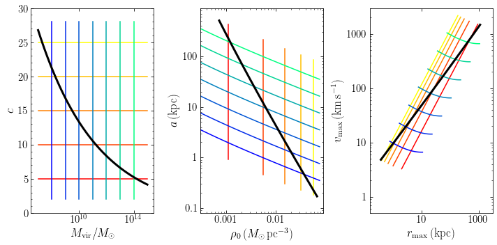
We see that lighter dark-matter halos are more concentrated than heavier halos, which results in an increase in the typical density \(\rho_0\) as the size \(a\) decreases. The behavior of the \(v_\mathrm{max}\) vs. \(r_\mathrm{max}\) relation mostly reflects the changing mass, which affects both \(v_\mathrm{max}\) and \(r_\mathrm{max}\) significantly. To allow the effects of changing concentration and virial-mass to be disentangled, the above figure also shows the location of a grid of halos with either concentration or virial mass held fixed (at \(c = 5, 10, \ldots\) or \(M_\mathrm{vir} = 10^8, 10^9, \ldots M_\odot\)). We see that, as expected from Equation \eqref{eq-nfw-rhoo-fromconc}, the typical density \(\rho_0\) only depends on concentration, while \(a\) depends on both virial mass and concentration. A wide range of concentrations only results in a small range of \(v_\mathrm{max}\) at a given \(r_\mathrm{max}\) compared to the range of \(v_\mathrm{max}\).