
6. Equilibria of collisionless stellar systems
The concept of equilibrium is of great importance in the observational study of galaxies. The basic reason for this comes from considering Newton’s second law: the gravitational force sets the acceleration of bodies, but does not directly set their positions and velocities. Yet, positions and velocities are all that we can observe for stars and gas in galaxies. Without further assumptions, positions and velocities themselves contain no direct information about the mass distribution in galaxies. That a dynamical system is in equilibrium is one of the most useful of such additional assumptions that one can make and one that allows us to probe the mass and orbital distributions of our own galaxy, the Milky Way, and of external galaxies in detail. We will start our study of dynamical equilibria in this chapter with some general results and their specific application to spherical systems.
Before starting on a mathematical description of dynamical equilibria, it is worth asking why we think this might be a good assumption. If you have ever watched a movie of a simulation of the formation of galaxies in the cosmological setting, you will know that galaxies are not in any equilibrium state when they form and keep being perturbed by infalling gas and galaxies. In section 6.1 below, we will demonstrate that the two-body relaxation time—on which timescale we can expect an equilibrium distribution to form through energy exchanges between pairs of bodies—is \(t_\mathrm{relax} \approx t_\mathrm{dyn}\,N/[8\,\ln N] \gg t_\mathrm{dyn}\) and is many orders of magnitude larger than the current age of the Universe for all galaxies. Thus, we cannot rely on two-body relaxation for galaxies to reach an equilibrium state.
Fortunately, there are non-collisional effects that drive stellar systems to an equilibrium state, in particular violent relaxation and phase mixing, and these effects act on the dynamical time scale rather than the two-body relaxation time scale (we discuss these effects in more detail in Chapter 18.3). Since the dynamical time is typically a few 100 Myr in galaxies, this means that galaxies have typically reached a quasi-equilibrium state at the present time. For any particular galaxy, this quasi-equilibrium can be perturbed, e.g., because of a merger with another galaxy, and the equilibrium assumption should therefore not be made blindly, but overall galaxies are close to being in dynamical equilibrium. An example of violent relaxation and phase-mixing for a one-dimensional, gravitating system is shown in the following animation:

What is shown is the phase-space distribution of \(N\) particles moving under the influence of their mutual gravity in one dimension. The system starts out in a very inhomogeneous state in phase-space—all particles have almost zero velocity over a wide range of positions—but over the course of just a few orbits, the distribution reaches a quasi-equilibrium.
Because the dynamical time behaves as \(t_\mathrm{dyn} \propto R/v\) and in galaxies \(v \approx\) constant or decreasing at large \(R\), the dynamical time at large distances (e.g., 100 kpc) becomes large and closer to the age of the Universe. The assumption of equilibrium is therefore more suspect in such places. This is also seen in the animation above, where phase-mixing is faster near the center of the mass distribution, because the dynamical time is shorter there.
We start this chapter with a detailed discussion of whether and on what timescales we can approximate a distribution of \(N\) bodies as a smooth distribution rather than a collection of point masses and derive an approximate expression for the relaxation timescale of stellar systems: the timescale on which interactions with the individual bodies that make up a smooth mass distribution are important. We then introduce one of the most basic relations for an equilibrium dynamical system: the virial theorem. The virial theorem is a blunt tool that relates the global spatial and kinematic properties to the overall gravitational potential and therefore does not lead to detailed knowledge about a galaxy’s mass distribution. However, it clearly shows the relation between kinematics, spatial scale, and gravitational mass that underlies all of the more sensitive methods that we will discuss later in this chapter and in later chapters. We then continue with a more rigorous discussion of the evolution of collisionless stellar systems and apply it to the equilibrium of spherical systems.
6.1. Collisionless vs. collisional dynamics
Galaxies are made up of large numbers \(N\) of stars and most probably even larger numbers of dark matter particles. For a typical galaxy like the Milky Way, the number of stars is \(N \approx 10^{11}\). One might think that the strong, gravitational interactions between individual stars are important drivers of the evolution of galaxies. In this case we would say that the dynamics is collisional (because collisions, even if they are not direct physical collisions, but simply near misses, are important). However, as we will see in this section, this is not the case and close encounters are not important. Galaxies are collisionless. More generally, we refer to effects as being “collisional” if they result from the fact that stellar systems are made up of a finite number of stars or gas clouds (or dark matter if the dark-matter mass is high).
The first thing of note is that the gravitational force drops off as \(1/r^2\) and is therefore a long-range force (a short-range force would be one where the force drops off exponentially or similarly fast). To a first approximation the density in galaxies is roughly constant and the total amount of gravitational force exerted on a star by a shell of stars with width \(\mathrm{d}r\) at a distance \(r\) is therefore \(\approx 1/r^2 \times 4\pi\,r^2\,\mathrm{d}r \propto \mathrm{d}r\): each shell contributes the same amount of force. Encounters between individual stars must be well within 1 pc to have a large effect and there are many more shells beyond 1 pc than within it. Therefore, the gravitational force on a star in a galaxy is dominated by the sum of the forces of distant stars rather than by the force from the nearest stars. Because the sum is over the contributions of \(\approx 10^{11}\) stars, this gravitational force is smooth in space and time and stars follow smooth orbits (we won’t say regular here, because that has a specific meaning as discussed in Section 4.4.3 and the smooth orbits of stars are not necessarily regular).
In more detail, we can compute the relaxation time as the time over which the combined effect of many close encounters has changed a star’s velocity by \(100\,\%\). To estimate the relaxation time of galactic systems, we will approximate them as consisting of \(N\) equal-mass bodies with mass \(m\) (for a total mass \(M = Nm\)) that are uniformly distributed over a sphere with radius \(R\). To first approximation, the effect of a two-body encounter is to deflect the orbits of the participating bodies and we can compute this deflection using the impulse approximation. In this approximation, we work in the coordinate frame centered on the first body and approximate the trajectory of the second body for the purpose of computing the deflection as following a straight line at constant speed \(v\) as shown in the following figure
[63]:
from galpy.potential import KeplerPotential
from galpy.orbit import Orbit
kp= KeplerPotential(normalize=1.)
r_init= 5.
v_init= 20.*kp.vcirc(r_init)
phi_init= numpy.pi-0.2
o= Orbit([r_init,v_init*numpy.cos(phi_init),
          -v_init*numpy.sin(phi_init),phi_init])
o.integrate(numpy.linspace(0.,1.2,101),kp)
# Location of first mass
o.plot(yrange=[-0.5,1.5])
plot([0.],[0.],'ko',ms=10.)
# Impule approx. trajectory
axhline(o.y(),ls='--')
# Impact parameter
plot([0.,0.],[0.,o.y()])
text(0.2,0.7,r'$b$',fontsize=20.,
     horizontalalignment='left',
     verticalalignment='center')
# theta line and label
force_arrow_t= 0.15
plot([0.,o.x(force_arrow_t)],[0.,o.y(force_arrow_t)])
text(-0.4,0.3,r'$\theta$',fontsize=20.,
     horizontalalignment='center',
     verticalalignment='center')
# Force arrow
gca().annotate("",
               xy=(o.x(force_arrow_t),o.y(force_arrow_t)-0.4),
               xytext=(o.x(force_arrow_t),o.y(force_arrow_t)),
              arrowprops=dict(arrowstyle="->"))
text(o.x(force_arrow_t)-0.1,o.y(force_arrow_t)-0.2,r'$F_\perp$',
     fontsize=20.,
     horizontalalignment='right',
     verticalalignment='center')
# x annotation
text(o.x(2.5*force_arrow_t),o.y()+0.05,
     r'$x$',
     fontsize=20.,
     horizontalalignment='center',
     verticalalignment='bottom')
gca()._frameon= False
gca().xaxis.set_visible(False)
gca().yaxis.set_visible(False);
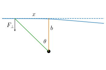
Thus, we approximate the true trajectory (the blue curve, from left to right) as following the dashed straight line. This line make a closest approach to the first body (the big dot) with a relative distance given by the impact parameter \(b\). We compute the deflection as the change in the component of the velocity perpendicular to the straight-line trajectory, \(\delta v_y\) in the example above. Following Newton’s second law (Equation 4.2), this change can be computed as
where \(F_\perp\) is the perpendicular component of the force, in this case given by
where \(\theta\) is the angle between the two lines indicated above. From trigonometry, we have that \(\cos \theta = b/\sqrt{x^2+b^2}\) and from the impulse approximation we have that \(x = vt\), such that the deflection becomes
where we used \(\tilde{x} = x/b\) and that \(\int_{-\infty}^\infty \mathrm{d} \tilde{x}\, {1 / (\tilde{x}^2+1)^{3/2}} = 2\). This is an often-used formula in different contexts and an easy way to remember it is to approximate the integral over force in Equation \eqref{eq-impulsedv-int} as the force at the impact parameter acting over the time \(\Delta T = 2b/v\) that it takes to cross from \(x=-b\) to \(x=b\)
This approximation works quite well in practice. For instance, for the example shown above, which has a noticeable deviation from the impulse approximation, we can compute the exact \(\delta v\) and the approximation (which we compute using that \(-GM/b = \Phi[b]\)):
[70]:
print("dv_exact = {:.5f}, dv_approx = {:.5f}, difference = {:.2f}%"\
      .format(o.vy(1.2), 2*kp(o.y(),0.)/o.vx(),
     (2*kp(o.y(),0.)/o.vx()-o.vy(1.2))/o.vy(1.2)*100.))
dv_exact = -0.22170, dv_approx = -0.22510, difference = 1.54%
Now consider a “subject” star passing through our galaxy of size \(R\). Crossing the galaxy, our “subject” star encounters approximately \(N/(\pi R^2) \times 2\pi\,b\mathrm{d}b = 2N\,b\mathrm{d}b/R^2\) stars in a shell of impact radius \(b\) (this is the surface density of stars \(N/(\pi R^2)\) times the area of the shell \(2\pi\,b\mathrm{d}b\)). If the impacts are at random angles, the velocity change from this shell will exhibit a random walk, leading the mean squared velocity to increase by
Integrating over all \(b\) gives
where \(\Lambda = b_{\mathrm{max}}/b_{\mathrm{min}}\), the minimum and maximum impact parameter. The minimum can be set to the impact parameter where the change in velocity from a single kick is equal to the velocity, \(v \approx \delta v = 2Gm/(b_{\mathrm{min}}v)\) or \(b_{\mathrm{min}} = 2Gm/v^2\). The maximum can be set to the size of the system, \(b_\mathrm{max} = R\). Then \(\Lambda = Rv^2/(2Gm)\).
We can now define and compute the relaxation time. The relaxation time is defined as the typical time it takes for individual encounters to change a star’s velocity (squared) by 100% (because the specific process that we are considering concerns interactions between two bodies, this process is known as two-body relaxation). First we compute the number of crossings necessary, from the equation for \(\langle \Delta v^2 \rangle\) per crossing:
We can simplify this expression by considering the circular velocity \(v_c\) at \(R\) as a typical velocity \(v\). In Chapter 3.3, we showed that \(v_c^2 = GM(<r)/r\) such that in this case \(v^2 = v_c^2=GNm/R\) or \(v^4 R^2 / (G^2\,m^2) = N^2\). Therefore, for a typical velocity we get
We can also simplify the expression for \(\Lambda = Rv^2/(2Gm)\) for this typical velocity: \(\Lambda = N/2 \approx N\). Thus,
Each crossing takes approximately a dynamical time \(t_\mathrm{cross} = 2\pi R/v\) and the relaxation time is therefore
For galaxies, \(N \approx 10^{11}\) and \(t_\mathrm{cross} \approx 100\) Myr. Therefore,
[4]:
trelax= 10.**11./8./numpy.log(10.**11)*100*u.Myr
print(trelax.to(10**10*u.Myr))
4.935164567082407 1e+10 Myr
or \(t_\mathrm{relax} \approx 5\times 10^{10}\) Myr, much much much larger than the age of the Universe (\(\approx 10^4\) Myr). There’s enough room in this argument for the effect of simplifying assumptions that any galaxy has a two-body relaxation time much larger than the age of the Universe. Therefore, we can safely say that galaxies are collisionless.
The situation in disk galaxies is slightly more complex than the above argument makes it appear. Even when only considering two-body relaxation, disks have shorter relaxation times than elliptical galaxies for the same \(N\). This is because the stars in disks are (a) packed closer together for the same size \(R\) (as they stay close to the mid-plane) and (b) move at smaller relative velocities with respect to each other, causing velocity kicks by Equation \(\eqref{eq-impulse-dv}\) to be larger. In fact, the two-body relaxation time in a razor-thin disk is \(t_\mathrm{relax} \approx t_\mathrm{dyn}\). But even after accounting for the thickness of a disk galaxy and its (small) internal velocity dispersion, one can show that the two-body relaxation time is longer than the age of the Universe for disk galaxies. Collisional effects, however, can also occur due to collective effects, for example, the tendency of disks to form spiral structure. Spiral structure can appear without any outside influence, caused simply by the finite number of stars and gas clouds that form a disk galaxy; spiral structure influences the orbits of stars in disks, which are then affected by a collisional effect. Similarly, stars in disks get deflected on their orbits by giant molecular clouds, which is also a direct collisional effect that changes the distribution function of stars. Most of these effects act on timescales larger than the dynamical time, thus, over a few dynamical times we can still mostly consider disks to be collisionless. We will come back to this question in later chapters.
The two-body relaxation argument fully breaks down for regions of high stellar density, such as within tens of parsecs of the centers of galaxies or in the cores of globular clusters. As we saw in Chapter 2.2.4, globular clusters have about \(N = 10^5\) stars in a region of a few pc. Their typical velocity is therefore \(v \approx 5\,\mathrm{km\,s}^{-1}\) and their crossing time \(t_\mathrm{cross} \approx 1\) Myr. Therefore,
[5]:
trelax= 10.**5./8./numpy.log(10.**5)*1*u.Myr
print(trelax.to(u.Gyr))
1.0857362047581296 Gyr
or
Two-body relaxation therefore plays a large role in the evolution of globular clusters. However, in these dense environments, it is still the case that \(t_\mathrm{relax} \gg t_\mathrm{dyn}\) and over a few dynamical times, we can still approximate the dynamics as being collionless. In the context of equilibrium models, this means that we can apply the tools from collionless modeling to the dynamics of galactic nuclei and globular clusters to investigate their instantaneous equilibrium state and relaxation slowly changes this (collisionless) equilibrium state through the slow effect of two-body interactions.
6.2. The virial theorem
The virial theorem relates the kinetic and potential energy of a system of bodies. We can derive different versions of the virial theorem, depending on whether we are dealing with a self-gravitating system of bodies (bodies moving under the influence of their mutual gravity) or a system of bodies orbiting within the potential due to an external mass distribution (for example, the system of globular clusters in the Milky Way, which orbit in the total Milky Way mass distribution and contribute almost no mass to this themselves). We can derive all different versions by starting from the virial quantity \(G\)
where \(w_i\) are a set of weights that is left arbitrary for now. Assuming that the system of \(N\) bodies is in equilibrium, we have that \(\mathrm{d} G / \mathrm{d} t = 0\) or
which we can write in terms of the gravitational field as
For \(w_i = m_i\), the masses of the bodies, the left-hand side of this equation equals twice the kinetic energy of the system.
If we now consider that the bodies are orbiting within a central, external point-mass potential, \(\Phi(r) = -G\,M/r\), then we get the following virial theorem
where \(r_i = |x_i|\) and the right-hand side is now minus the potential energy. The mass of the system is therefore
This result holds for any weighting \(w_i\), although how good of an estimator the right-hand side is for the mass will strongly depend on how the bodies are weighted (for example, setting all \(w_i\) but one equal to zero will make this a very noisy estimator! Of course, then the assumption that \(\mathrm{d} G / \mathrm{d} t = 0\) also breaks down). The simplest choice for the weights is \(w_i=1\).
Alternatively, we can work out Equation \(\eqref{eq-virial-verygeneral}\) for a set of self-gravitating bodies. In that case, \(\vec{g}(\vec{x}_i) = \sum_{j \neq i} G\,m_j\,(\vec{x}_i-\vec{x}_j)/|\vec{x}_i-\vec{x}_j|^3\). The right-hand side of Equation \(\eqref{eq-virial-verygeneral}\) can then be written as
If we then set \(w_i = m_i\), this can be simplified to
which is again minus the potential energy of the system. The virial theorem for self-gravitating systems is therefore
If all bodies have the same mass \(m\) and the total mass is \(M = Nm\) then we can estimate the mass as
Equations \(\eqref{eq-virial-mass-kepler}\) and \(\eqref{eq-virial-mass-selfgrav}\) both make it clear that under the assumption of equilibrium, the mass of a stellar system can be obtained by balancing the spread in velocities (the kinetic energy) with an appropriate weighting of the spread in positions (the potential energy). This makes sense: if we guess a mass \(M\) that is too low, then the observed velocities would be too high and the system would in the future quickly spread out and thus not be in equilibrium; if on the other hand, we guess a mass that is too high, the velocities would appear low and the system will quickly collapse to occupy a smaller volume. For the correct mass \(M\), both the spread in velocities and in positions can be maintained over time.
The virial theorem in the form above is also known as the scalar virial theorem, to distinguish it from more detailed forms of the virial theorem like the tensor virial theorem that we will discuss in Chapter 15.1 in the context of elliptical galaxies. There, we also discuss how to generalize the virial theorem to continuous, collisionless systems. When we set \(w_i = m_i\), both the external-point-mass-potential and self-gravitating cases of the virial theorem can be written as
where \(K\) is the kinetic energy and \(W\) is the potential energy. Using that the total energy \(E = K + W\), we can also write this as
Let’s use these virial estimators to estimate the mass of the Milky Way using globular clusters from the Harris 1996 catalog (2010 edition) catalog that we discussed in Chapter 2.2.4. First we write a function to download and read the catalog, which we save in a cache directory $HOME/.galaxiesbook/cache/harris (note that the catalog is
somewhat difficult to read, which is why the harris_read function below is quite complicated…):
[74]:
# harris.py: download, parse, and read the Harris
# Milky-Way globular cluster catalog
# Include all necessary imports to make this cell self-contained
import sys
import os, os.path
import shutil
import subprocess
import tempfile
import numpy
import pandas
_MAX_DOWNLOAD_NTRIES= 2
_ERASESTR= "                                                                                "
_CACHE_BASEDIR= os.path.join(os.getenv('HOME'),'.galaxiesbook','cache')
_CACHE_HARRIS_DIR= os.path.join(_CACHE_BASEDIR,'harris')
_HARRIS_URL= 'http://physwww.mcmaster.ca/~harris/mwgc.dat'
def harris_read(verbose=False):
    """
    NAME:
       read
    PURPOSE:
       read and parse the Harris Milky-Way globular cluster catalog
    INPUT:
       verbose= (False) if True, print some progress updates
    OUTPUT:
       pandas DataFrame with the catalog
    HISTORY:
       2017-07-26 - Started - Bovy (UofT)
    """
    filePath= os.path.join(_CACHE_HARRIS_DIR,'mwgc.dat')
    _download_harris(filePath,verbose=verbose)
    with open(filePath,'r') as harrisfile:
        lines= harrisfile.readlines()
        # 1st part: 72-229, 2nd part: 252-409, 3rd part: 433-590
        ids= lines[72:229]
        metals= lines[252:409]
        vels= lines[433:590]
        # Parse into dict
        ids_dict= {'ID': [],
                   'Name': [],
                   'RA': numpy.empty(len(ids)),
                   'DEC': numpy.empty(len(ids)),
                   'L': numpy.empty(len(ids)),
                   'B': numpy.empty(len(ids)),
                   'R_Sun': numpy.empty(len(ids)),
                   'R_gc': numpy.empty(len(ids)),
                   'X': numpy.empty(len(ids)),
                   'Y': numpy.empty(len(ids)),
                   'Z': numpy.empty(len(ids)),
                   '[Fe/H]': numpy.empty(len(ids)),
                   'wt': numpy.empty(len(ids)),
                   'E(B-V)': numpy.empty(len(ids)),
                   'V_HB': numpy.empty(len(ids)),
                   '(m-M)V': numpy.empty(len(ids)),
                   'V_t': numpy.empty(len(ids)),
                   'M_V,t': numpy.empty(len(ids)),
                   'U-B': numpy.empty(len(ids)),
                   'B-V': numpy.empty(len(ids)),
                   'V-R': numpy.empty(len(ids)),
                   'V-I': numpy.empty(len(ids)),
                   'spt': ['---' for ii in range(len(ids))],
                   'ellip': numpy.empty(len(ids)),
                   'v_r': numpy.empty(len(ids)),
                   'v_r_unc': numpy.empty(len(ids)),
                   'v_LSR': numpy.empty(len(ids)),
                   'sig_v': numpy.empty(len(ids)),
                   'sig_v_unc': numpy.empty(len(ids)),
                   'c': numpy.empty(len(ids)),
                   'r_c': numpy.empty(len(ids)),
                   'r_h': numpy.empty(len(ids)),
                   'mu_V': numpy.empty(len(ids)),
                   'rho_0': numpy.empty(len(ids)),
                   'lg(tc)': numpy.empty(len(ids)),
                   'lg(th)': numpy.empty(len(ids)),
                   'core_collapsed': numpy.zeros(len(ids),dtype='bool')}
        # Parse first part
        rest_keys= ['L','B','R_Sun','R_gc','X','Y','Z']
        for ii in range(len(ids)):
            # Parse ID and Name
            ids_dict['ID'].append(ids[ii][:10].strip())
            name= ids[ii][10:25].strip()
            if name == '': ids_dict['Name'].append('---')
            else: ids_dict['Name'].append(name)
            # Parse RA and Dec, Harris (l,b) don't seem exactly right...
            hms= ids[ii][25:36].split() # hour, min, sec
            ids_dict['RA'][ii]=\
                int(hms[0])*15.+int(hms[1])/4.+float(hms[2])/240.
            hms= ids[ii][38:49].split() # deg, arcmin, arcsec
            sgn= -1 if ids[ii][38] == '-' else 1
            ids_dict['DEC'][ii]=\
                int(hms[0])+sgn*(int(hms[1])/60.+float(hms[2])/3600.)
            # Split the rest
            rest= ids[ii][49:].split()
            for r,k in zip(rest,rest_keys): ids_dict[k][ii]= float(r.strip())
        # Parse second part
        idx_arr= numpy.arange(len(ids))
        for ii in range(len(metals)):
            # Not sure whether I can assume that they are in order
            idname= metals[ii][:10].strip()
            idx= idx_arr[\
                numpy.core.defchararray.equal(ids_dict['ID'],idname)][0]
            ids_dict= _parse_float_entry(ids_dict,'[Fe/H]',idx,
                                         metals[ii][13:18].strip())
            ids_dict= _parse_float_entry(ids_dict,'wt',idx,
                                         metals[ii][19:21].strip())
            ids_dict= _parse_float_entry(ids_dict,'E(B-V)',idx,
                                         metals[ii][24:28].strip())
            ids_dict= _parse_float_entry(ids_dict,'V_HB',idx,
                                         metals[ii][29:34].strip())
            ids_dict= _parse_float_entry(ids_dict,'(m-M)V',idx,
                                         metals[ii][35:40].strip())
            ids_dict= _parse_float_entry(ids_dict,'V_t',idx,
                                         metals[ii][42:46].strip())
            ids_dict= _parse_float_entry(ids_dict,'M_V,t',idx,
                                         metals[ii][48:53].strip())
            for k,si,ei in zip(['U-B','B-V','V-R','V-I'],
                               [56,62,68,74],[60,66,72,78]):
                ids_dict= _parse_float_entry(ids_dict,k,idx,
                                             metals[ii][si:ei].strip())
            ids_dict['spt'][idx]= metals[ii][80:82].strip()
            ids_dict= _parse_float_entry(ids_dict,'ellip',idx,
                                         metals[ii][86:].strip())
        # Parse third part
        idx_arr= numpy.arange(len(ids))
        for ii in range(len(vels)):
            # Not sure whether I can assume that they are in order
            idname= vels[ii][:10].strip()
            idx= idx_arr[\
                numpy.core.defchararray.equal(ids_dict['ID'],idname)][0]
            for k,si,ei in zip(['v_r','v_r_unc','v_LSR','sig_v','sig_v_unc',
                                'c','r_c','r_h','mu_V','rho_0',
                                'lg(tc)','lg(th)'],
                               [13,21,27,37,43,50,59,66,73,80,88,93],
                               [19,25,33,41,47,54,64,70,78,85,91,98]):
                ids_dict= _parse_float_entry(ids_dict,k,idx,
                                             vels[ii][si:ei].strip())
            if vels[ii][56] == 'c': ids_dict['core_collapsed'][idx]= True
        return pandas.DataFrame(ids_dict)

def _parse_float_entry(ids_dict,key,idx,val):
    try:
        ids_dict[key][idx]= float(val)
    except ValueError:
        ids_dict[key][idx]= numpy.nan
    return ids_dict

def _download_harris(filePath,verbose=False):
    if not os.path.exists(filePath):
        _download_file(_HARRIS_URL,filePath,verbose=verbose)
    return None

def _download_file(downloadPath,filePath,verbose=False,spider=False,
                   curl=False):
    sys.stdout.write('\r'+"Downloading file %s ...\r" \
                         % (os.path.basename(filePath)))
    sys.stdout.flush()
    try:
        # make all intermediate directories
        os.makedirs(os.path.dirname(filePath))
    except OSError: pass
    # Safe way of downloading
    downloading= True
    interrupted= False
    file, tmp_savefilename= tempfile.mkstemp()
    os.close(file) #Easier this way
    ntries= 1
    while downloading:
        try:
            if curl:
                cmd= ['curl','%s' % downloadPath,
                      '-o','%s' % tmp_savefilename,
                      '--connect-timeout','10',
                      '--retry','3']
            else:
                cmd= ['wget','%s' % downloadPath,
                      '-O','%s' % tmp_savefilename,
                      '--read-timeout=10',
                      '--tries=3']
            if not verbose and curl: cmd.append('-silent')
            elif not verbose: cmd.append('-q')
            if not curl and spider: cmd.append('--spider')
            subprocess.check_call(cmd)
            if not spider or curl: shutil.move(tmp_savefilename,filePath)
            downloading= False
            if interrupted:
                raise KeyboardInterrupt
        except subprocess.CalledProcessError as e:
            if not downloading: #Assume KeyboardInterrupt
                raise
            elif ntries > _MAX_NTRIES:
                raise IOError('File %s does not appear to exist on the server ...' % (os.path.basename(filePath)))
            elif not 'exit status 4' in str(e):
                interrupted= True
            os.remove(tmp_savefilename)
        finally:
            if os.path.exists(tmp_savefilename):
                os.remove(tmp_savefilename)
        ntries+= 1
    sys.stdout.write('\r'+_ERASESTR+'\r')
    sys.stdout.flush()
    return None
We now load the catalog and convert the positions to the Galactocentric frame:
[75]:
import astropy.units as u
import astropy.constants as const
import astropy.coordinates as apycoords
gcdata= harris_read()
c= apycoords.SkyCoord(ra=gcdata['RA'],
                      dec=gcdata['DEC'],
                      distance=gcdata['R_Sun'],
                      unit=(u.deg,u.deg,u.kpc),
                      frame='icrs')
gc_frame= apycoords.Galactocentric(galcen_distance=8.1*u.kpc,
                                   z_sun=25.*u.pc)
gc = c.transform_to(gc_frame)
gc.representation_type = 'spherical'
To be in a regime where the assumption of spherical symmetry is closer to being correct, we only select clusters at distances well beyond the disk, \(r > 20\,\mathrm{kpc}\). We can then estimate the mass of the Milky Way using the estimator from Equation \(\eqref{eq-virial-mass-kepler}\), assuming that the globular clusters are test particles in a point-mass potential. Observations of the proper motions of globular clusters are difficult, so we will estimate \(\sum_i |\vec{v}_i|^2\) from just the line-of-sight velocities under the assumption that (a) the velocity distribution is Gaussian and isotropic and (b) the line-of-sight velocity (approximately corrected for the Sun’s motion with respect to the solar neighborhood to \(v_\mathrm{LSR}\)) is approximately equal to the Galactocentric radial velocity; then we can estimate \(\sum_i |\vec{v}_i|^2\) as \(3\sum_i v_\mathrm{LSR}^2\). Putting this together with the Galactocentric distances, we find
[8]:
indx= (gc.distance > 20.*u.kpc)*(True^numpy.isnan(gcdata['v_LSR']))
M_est= (3.*numpy.sum(gcdata['v_LSR'][indx]**2.)\
        *(u.km/u.s)**2\
       /numpy.sum(1./gc.distance[indx])/const.G)
print("""For a point-mass central potential,
    with %i GCs with median distance %.0f kpc
    the mass is %.2f 10^12 Msun""" % \
    (numpy.sum(indx),
     numpy.median(gc.distance[indx]).to(u.kpc).value,
     M_est.to(10**12*u.Msun).value))
For a point-mass central potential,
    with 19 GCs with median distance 35 kpc
    the mass is 0.45 10^12 Msun
If instead we assume that the globular clusters form a self-gravitating system and similarly apply Equation \(\eqref{eq-virial-mass-selfgrav}\) we get
[9]:
mutual_dist= \
 (numpy.atleast_2d(gc.distance[indx]).T-gc.distance[indx])
mutual_dist[numpy.diag_indices(numpy.sum(indx))]= 0.
mutual_dist= numpy.triu(mutual_dist)
M_est= (3.*numpy.sum(gcdata['v_LSR'][indx]**2.)*(u.km/u.s)**2\
        /numpy.sum(1./numpy.fabs(mutual_dist)[mutual_dist > 0])\
        *numpy.sum(indx)/const.G)
print("""For a self-gravitating system,
    with %i GCs with median distance %.0f kpc
    the mass is %.2f 10^12 Msun""" % \
    (numpy.sum(indx),
     numpy.median(gc.distance[indx]).to(u.kpc).value,
     M_est.to(10**12*u.Msun).value))
For a self-gravitating system,
    with 19 GCs with median distance 35 kpc
    the mass is 0.17 10^12 Msun
We see that there is only a factor of two difference between the two estimators, so no matter what estimator we use, we always find a large mass (larger than the total mass of stars and gas by at least a factor of two). It is also clear from this that the globular clusters cannot form a self-gravitating system: for the self-gravitating estimator to make sense, each globular cluster would have to have a mass of about \(10^{10}\,M_\odot\), so their mass-to-light ratio would have to be \(M/L \gtrsim 10^4\)!
Comparing the estimate assuming a point-mass potential with the enclosed-mass profile for the Milky Way that we discussed in Chapter 2.2.1, we see that the virial estimator is not that far off from our current best knowledge (it is about 30% higher than the best estimate), even though the virial estimator is highly simplified. This demonstrates the power and simplicity of equilibrium modeling.
6.3. The collisionless Boltzmann equation
To go beyond the virial theorem, we now study the evolution of gravitational systems made up of large numbers of particles in more depth. The fundamental equation describing collisionless systems is the collisionless Boltzmann equation. This equation describes the behavior of the distribution function \(f(\vec{x},\vec{v},t)\) of bodies moving under the influence of gravity. The distribution function gives the number of bodies in a small volume of phase space at a given time \(t\): \(\mathrm{d}N(\vec{x},\vec{v},t) \propto f(\vec{x},\vec{v},t)\,\mathrm{d}\vec{x}\,\mathrm{d}\vec{v}\), with the proportionality set by how one chooses to normalize \(f\). We will use \(\vec{w} \equiv (\vec{x},\vec{v})\) to denote phase-space coordinates. The “collisionless” assumption implies that this “one-body” distribution function fully describes the system, that is, that there are no correlations between the number of bodies at different phase-space positions. Said another way, the assumption is that the presence of a body at one position does not affect the probability of seeing a body at another position. Thus, the \(N\)-body distribution function \(f^{(N)}(\vec{w}_1,\vec{w}_2,\ldots,\vec{w}_N,t)\) is simply given by
for all \(N\). We further normalize \(f(\vec{w},t)\) such that \(\int \mathrm{d}\vec{w}\,f(\vec{w},t) = 1\) for all times \(t\). We can then consider what happens to the total number of stars \(N(\mathcal{V},t) = \int_{\mathcal{V}} \mathrm{d}\vec{w}\, f(\vec{w},t)\) in a volume \(\mathcal{V}\) of phase space with a surface \(S\). As time passes, the number of bodies in \(\mathcal{V}\) will change as \(\mathrm{d} N(\mathcal{V},t) / \mathrm{d} t = \int_\mathcal{V} \mathrm{d}\vec{w}\,\partial f(\vec{w},t) / \partial t\). Assuming that no bodies are created or removed inside the volume, this change happens because stars leave and enter \(\mathcal{V}\) through the boundary \(S\) at a rate of \(f(\vec{w},t)\,\dot{\vec{w}}_\perp\) (the subscript \(\perp\) denotes that the flow is perpendicular to the surface, with a positive rate defined as pointing outward). The total flow across the surface is the integral over the entire surface of this flow: \(\oint_S \mathrm{d} S\, f(\vec{w},t)\,\dot{\vec{w}}_\perp\), and because the number of stars must be conserved, this must be equal to the change in the number of stars in \(\mathcal{V}\):
Using the divergence theorem we can write the integral on the right-hand side as a volume integral as well
Because this equation must hold for any volume \(\mathcal{V}\), it must be the case that
which is the continuity equation for the phase-space density. Now let’s work out the gradient in terms of the cartesian position and momentum coordinates \((\vec{x},\vec{v})\)
Because \(\partial \dot{\vec{x}} / \partial \vec{x} = \partial \dot{\vec{v}} / \partial \vec{v} = 0\) this becomes
which is the collisionless Boltzmann equation. This equation in fact holds for any set of canonical coordinates \((\vec{q},\vec{p})\). The derivation up to Equation \(\eqref{eq-coll-boltzmann-penultstep}\) is the same, because \(f(\vec{q},\vec{p},t) = f(\vec{x},\vec{v},t)\) (which in turn follows from the fact that \(\mathrm{d}\vec{q}\,\mathrm{d}\vec{p} = \mathrm{d}\vec{x}\,\mathrm{d}\vec{v}\) for any set of canonical coordinates as we showed in Section 4.4.2) . The last step leads to
in this case because \(\partial \dot{\vec{q}} / \partial \vec{q} = -\partial \dot{\vec{p}} / \partial \vec{p}\) from Hamilton’s equations. Equation \(\eqref{eq-collisionless-boltzmann}\) makes it much easier to write down the collisionless Boltzmann equation in coordinate systems other than cartesian coordinates. In cartesian coordinates, we can re-write Equation \(\eqref{eq-collisionless-boltzmann-cartesian}\) as
by using Newton’s second law. For general canonical coordinates \((\vec{q},\vec{p})\), we have a similar equation using Hamilton’s equations
The collisionless Boltzmann equation describes the evolution of any collisionless system, not just those that are in equilibrium. It is the fundamental equation of collisionless dynamics and the equation that is solved by \(N\)-body simulations. If the system under consideration is self-gravitating, the density of stars sources the potential and the Poisson equation becomes an additional evolution equation that relates the gravitational potential and the distribution function
where \(M\) is the total mass of the system (because of our convention that \(\int \mathrm{d}\vec{x}\mathrm{d}\vec{v}\,f(\vec{x},\vec{v},t) = 1\), we have that \(\rho(\vec{x},t) = M\,\int \mathrm{d} \vec{v}\,f(\vec{x},\vec{v},t)\) such that \(\int \mathrm{d}\vec{x}\, \rho(\vec{x},t) = M\,\int \mathrm{d}\vec{x}\,\mathrm{d} \vec{v}\,f(\vec{x},\vec{v},t) = M\)).
Such a system is a self-consistent system. But the collisionless Boltzmann equation does not only apply to self-consistent systems, it more generally describes the evolution of a subset of bodies orbiting in a general smooth mass distribution that they do not necessarily contribute much mass to (for example, the globular cluster system in the Milky Way; see above).
For a system in equilibrium, the number of stars in a given region of phase-space does not change, so \(\partial f(\vec{x},\vec{v},t) / \partial t = 0\). For such systems, the collisionless Boltzmann equation reduces to
This is the equilibrium collisionless Boltzmann equation. In the next sections we study solutions and properties of this equilibrium equation.
Before continuing, we will consider one more corollary of the collisionless Boltzmann equation. The collisionless Boltzmann equation describes how the phase-space density \(f(\vec{x},\vec{v})\) behaves in general. But we can also consider how \(f(\vec{x},\vec{v})\) evolves along the orbit of a body. The time evolution of \(f(\vec{x},\vec{v})\) along the orbit is given by
because the right-hand side is simply the expression in the collisionless Boltzmann equation \(\eqref{eq-collisionless-boltzmann}\). Thus, we find Liouville’s theorem: the phase-space density is conserved along orbital trajectories. This is a very useful property of Hamiltonian systems.
Let’s look at an example of Liouville’s theorem. In a simple one-dimensional potential (one-dimensional such that we can directly visualize the two-dimensional phase space), we start with a set of \(n\) initial points \((x_i,v_i)\) along the edge of a small circular area. We then integrate all of these orbits for some time and plot the evolution of the phase-space area spanned by the \((x_i[t],v_i[t])\) at different times \(t\).
[81]:
from galpy.orbit import Orbit
from galpy.potential import LogarithmicHaloPotential
from galpy.util import plot as galpy_plot
from matplotlib import pyplot
from matplotlib.patches import Polygon
from matplotlib.collections import PatchCollection
# Simple one-dimensional potential
lp= LogarithmicHaloPotential(normalize=1.).toVertical(1.)
# Trace out initially circular phase-space area
npoints= 101
theta= numpy.linspace(0,2.*numpy.pi,npoints,endpoint=True)
phase_space_radius= 0.15
xs= phase_space_radius*numpy.cos(theta)+1.
vs= phase_space_radius*numpy.sin(theta)+1
# Integrate all points along the edge of the area
os= [Orbit([x,v]) for x,v in zip(xs,vs)]
nts= 11
ts= numpy.linspace(0.,10.5,nts)
[o.integrate(ts,lp) for o in os]
# Create matplotlib polygons to represent area at each time
patches= []
for ii,t in enumerate(ts):
    polygon= Polygon(numpy.array([[o.x(t),o.vx(t)] for o in os]),
                     closed=True)
    patches.append(polygon)
p= PatchCollection(patches,alpha=1.)
galpy_plot.start_print(axes_labelsize=17.,text_fontsize=12.,
                       xtick_labelsize=15.,ytick_labelsize=15.)
fig, ax= pyplot.subplots(figsize=(10,5))
ax.set_aspect('equal')
ax.add_collection(p)
xlim(-3.,3)
ylim(-1.5,1.5)
xlabel(r'$x$')
ylabel(r'$v$')
pyplot.text(2.1,1.2,r'$t=0$',size=18.)
pyplot.show();
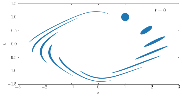
The initially circular phase-space area quickly gets stretched out in one direction and squashed in the other and then gets deformed as time progresses. But it is clear that the total area is conserved: the area becomes progressively thinner, but also gets longer in such a way that the total area does not change.
6.4. The Jeans equations
6.4.1. Generalities
As a partial differential equation, Equation \(\eqref{eq-collisionless-boltzmann-equil}\) admits a wide range of solutions depending on the initial and boundary conditions of the problem being considered. We will discuss two applications of solving the collisionless Boltzmann equation here: (i) to find an equilibrium distribution \(f(\vec{x},\vec{v})\) for a given potential \(\Phi(\vec{x})\) and a given density \(\nu(\vec{x})\) (which may or may not source the potential through the Poisson equation; we write the density as \(\nu(\vec{x})\) in case this density is not the full mass density that sources the potential and which we denote as \(\rho(\vec{x})\)) and (ii) to measure the mass distribution \(\Phi(\vec{x})\) from observations of \((\vec{x},\vec{v})\) assuming equilibrium.
In the next section we will discuss direct solutions of \(f(\vec{x},\vec{v})\) of the collisionless Boltzmann equation, but in this section we first discuss a different and somewhat simpler approach. Rather than working with the collisionless Boltzmann equation \(\eqref{eq-collisionless-boltzmann}\) itself, we can multiply this equation with \(\vec{x}^\alpha\) or \(\vec{v}^\beta\) for some \((\alpha,\beta)\) and integrate over a part of phase-space to obtain moment equations which are known as Jeans equations.
The Jeans equations involve moments of the distribution function. Because astronomical observations are typically performed at a fixed \(\vec{x}\) (or at least at a fixed two-dimensional location on the sky), multiplying the collisionless Boltzmann equation by \(\vec{v}^\beta\) and integrating over all components of the velocity most directly connects to observable quantities. Typical moments that we will consider are the spatial number density \(\nu(\vec{x})\)
and the mean velocity \(\bar{\vec{v}}(\vec{x})\)
which has components \(\bar{v}_i\). We also consider the velocity dispersion tensor \(\vec{\sigma}(\vec{x})\) with components \(\sigma_{ij}(\vec{x})\)
Higher-order moments are defined in a similar manner and quickly become much more complex. By multiplying Equation \eqref{eq-collisionless-boltzmann-cartesian} (or its other forms) by \(\vec{v}^\beta\) and integrating over \(\vec{v}\), we can derive a set of Jeans equations that relate these moments. For example, integrating Equation \eqref{eq-collisionless-boltzmann-cartesian-wpot} over \(\vec{v}\) we obtain
The final term vanishes after applying the divergence theorem (assuming that \(f\) goes to zero as \(\vec{v} \rightarrow \infty\)) and the partial derivatives in the first two terms may be taken outside of the integral, such that this equation becomes
which is the continuity equation for the density. Thus, we see that this Jeans equation involves both the density \(\nu(\vec{x})\) and the three-dimensional mean velocity \(\bar{\vec{v}}(\vec{x})\). This single equation therefore does not provide enough information to solve for the mean velocity given the density. Similarly multiplying Equation \eqref{eq-collisionless-boltzmann-cartesian-wpot} by a component of the velocity \(v_j\), integrating over all \(\vec{v}\), and subtracting the result from \(\bar{v}_j\) times the continuity equation leads to the following equation
for all \(i,j\) (we have dropped the functional dependence on \(\vec{x}\) of all of the quantities involved for notational simplicity). This Jeans equation therefore relates the density, mean velocity, and velocity dispersion tensor (as well as the gravitational field). However, while we now have an additional three equations, we have introduced the six components of the velocity dispersion tensor and there are therefore still not enough equations to solve for all of the kinematic quantities. Continuing this procedure by multiplying by higher powers of velocity (e.g., \(v_i\,v_j\)) and integrating over velocity leads to Jeans equations that involve higher and higher moments of the distribution function and at no point does the system of equations close, i.e., provide enough equations to uniquely solve for all kinematic properties. It is therefore not possible to solve for all of the moments of the distribution function through the Jeans equation starting from a known \(\Phi(\vec{x})\) and \(\nu(\vec{x})\) without additional assumptions to close the set of equations. This is a physical impossibility, not just a mathematical one: there are infinitely many equilibrium distribution functions in any gravitational potential and this continues to be the case when we demand that the distribution function sources the gravitational potential sources through Equation \eqref{eq-spherequil-selfconsist} (except for pathological cases such as the point-mass potential).
The Jeans equations are nevertheless useful, because they involve quantities that are readily observable, such as the spatial density (which can be traced through the surface brightness or through star counts), the mean velocity, and the velocity dispersion. By combining these observables with assumptions about the distribution function to close the system of equations, we can therefore constrain \(\Phi(\vec{x})\). In the Milky Way in particular, it is (in principle) possible to measure all moments of the velocity distribution (because we can obtain full six-dimensional phase-space information for many stars) and in this case the Jeans equation leads to direct measurements of \(\Phi(\vec{x})\) without any closure assumptions.
6.4.2. The spherical Jeans equation
To demonstrate the usefulness of the Jeans equations, we will start by considering them for spherical systems. To derive the spherical Jeans equation, we start from Equation \(\eqref{eq-collisionless-boltzmann-equil}\) and we use the Hamiltonian appropriate for spherical coordinates \(\vec{q} = (r,\phi,\theta)\) (we also set \(m=1\)). This Hamiltonian has momenta \(\vec{p}\) that are easily derived by writing down the Lagrangian in spherical coordinates:
The Hamiltonian itself is
Using \(\dot{\vec{q}} = \partial H / \partial \vec{p}\) and \(\dot{\vec{p}} = -\partial H / \partial \vec{q}\) we find that Equation \(\eqref{eq-collisionless-boltzmann}\) becomes
We now multiply this by \(p_r\) and integrate over all \((p_r,p_\phi,p_\theta)\) using that \(\mathrm{d}p_r\,\mathrm{d}p_\phi\,\mathrm{d}p_\theta = r^2\,\sin\theta\,\mathrm{d}v_r\, \mathrm{d}v_\phi\,\mathrm{d}v_\theta\) and using partial integration to deal with the derivatives of \(f\) with respect to the momenta. In bringing derivatives outside of integrals, it is important to remember the quantities held constant for each partial derivative: the partial derivatives are for the canonical set of coordinates \((r,\phi,\theta,p_r,p_{\phi},p_{\theta})\) and a derivative like \(\partial / \partial r\) therefore in particular keeps the momenta constant and can therefore be brought outside of the momentum integral. In the end, we obtain
As we will see below, for a spherical system the equilibrium distribution function can only be a function of energy and angular momentum, of which only the energy depends on \(p_r\) and it does so in a quadratic manner. This implies that all odd moments of \(v_r\) must vanish, in particular \(\overline{v_r\,v_\theta} = \overline{v_r\,v_\phi} = 0\) and we can therefore simplify Equation \(\eqref{eq-spher-jeans-penult}\) to
or
We can define a parameter \(\beta\) that quantifies the amount of orbital anisotropy (the difference in the velocity distribution in different directions)
where the first line is the actual definition and the second line follows if we assume that the system has no net rotation. This parameter measures a system’s radial anisotropy in the following sense: if the spread in the motions in the radial direction \(r\) is the same as that in the tangential directions \((\phi,\theta)\) then \(\sigma_r = \sigma_\phi = \sigma_\theta\), \(\beta = 0\), and the system is isotropic; if the spread in radial motions is much larger than that in the perpendicular dimensions, \(\sigma_r \gg \sigma_\theta, \sigma_\phi\) and \(\beta \rightarrow 1\) and we say that the system is radially biased; if all orbits are circular, \(\sigma_r = 0\), \(\beta = -\infty\), and we say that the system is tangentially biased (note the unfortunate asymmetry inherent in this definition: the radially biased range for \(\beta\) is \(0 < \beta \leq 1\), while the tangentially biased range is \(-\infty \leq \beta < 0\)). The anisotropy parameter in a realistic system will in general depend on radius \(\beta = \beta(r)\).
In terms of this anisotropy parameter, we can write the spherical Jeans equation for a non-rotating system as
We can also directly express the enclosed-mass profile in terms of the density \(\nu\), the velocity dispersion \(\sigma_r = \sqrt{\overline{v_r^2}}\)—this holds because \(\overline{v_r} = 0\), because all odd moments of \(v_r\) vanish (see above)—and the anisotropy \(\beta\), because \(G\,M(<r)/r^2 = \mathrm{d}\Phi(r) / \mathrm{d} r\)
For spherical systems we can therefore directly measure the enclosed-mass profile from measurements of the radial velocity dispersion and the logarithmic decline of the density times the dispersion squared as long as the anisotropy is known or can be constrained. Unfortunately, for most systems of interest it is difficult to measure the anisotropy, because it requires measurements of at least two of the velocity dimensions, while we typically can only access one through measurements of the line-of-sight velocity (proper motions can only be measured within a few to tens of kpc from the Sun and are therefore inaccessible at the present time for extra-galactic systems or for the far reaches of the Milky Way). This gives rise to the famous mass–anisotropy degeneracy in galactic mass modeling. One way around this is to derive higher-order spherical Jeans equations, which make use of higher-order moments of the velocity distribution (but as we discussed above, these equations do not close and assumptions are always necessary to make the equations work with only the line-of-sight velocity).
When the anisotropy \(\beta\) is assumed to be constant and the system is not rotating, the spherical Jeans equation can be integrated to give
or also
The integration range is such that the solution satisfies the boundary condition that \(\lim_{r\rightarrow\infty}\nu\,\sigma_r^2 = 0\).
If \(\beta = \beta(r)\) and the system is not rotating, we can consider Equation \(\eqref{eq-spher-jeans-anisotropy}\) to be a differential equation for \(\nu\,\overline{v^2_r} = \nu\,\sigma_r^2\). Differential equations of the type in Equation \(\eqref{eq-spher-jeans-anisotropy}\) can be solved in terms of an integrating factor
where \(r_0\) is some arbitrary lower limit, because then Equation \(\eqref{eq-spher-jeans-anisotropy}\) can be written as
This equation can be solved through direct integration of both sides and in the end we have that
These solutions for constant or radially-varying \(\beta\) can be used to determine the velocity dispersion for a mass model \(M(<r')\) and an assumed \(\beta(r)\) when the three-dimensional density is known. In external systems we can typically only measure the two-dimensional surface-brightness profile \(I(R)\) or the projected two-dimensional stellar density \(\Sigma(R)\); we discuss how to deal with this in Jeans analyses in Chapter 7.4.
As an example of the spherical Jeans equation, we can compute the velocity dispersion for a dark-matter halo modeled as an NFW profile for different values of the anisotropy. We use a halo with virial mass \(M_\mathrm{vir} = 10^{12}\,M_\odot\) and a concentration of 8.37 (following the Dutton & Macciò 2014 relation as in Chapter 3.4.6 with \(h=0.671\)). The radial velocity dispersion out to the virial radius is shown in the figure below:
[165]:
from galpy.potential import NFWPotential
from galpy.df import jeans
from matplotlib.cm import winter
from matplotlib.ticker import FuncFormatter
np= NFWPotential(mvir=1,conc=8.37,
                   H=67.1,overdens=200.,wrtcrit=True,
                   ro=8.,vo=220.)
betas= [-5.,-3.,-1.,-0.5,0.,0.5,0.75,0.99]
rs= numpy.geomspace(0.1,np.rvir(H=67.1,overdens=200.,wrtcrit=True).to_value(u.kpc),41)*u.kpc
figsize(10,5)
for ii,beta in enumerate(betas):
    sigs= numpy.array([jeans.sigmar(np,r,beta=beta).to_value(u.km/u.s) for r in rs])
    subplot(1,2,1)
    galpy_plot.plot(rs.to_value(u.kpc),
                    sigs,
                    semilogx=False,
                    xrange=[0.,270.],
                    yrange=[0.,200.],
                    gcf=True,
                    overplot=beta!=betas[0],
                    color=winter(ii/(len(betas)-1.)),
                    xlabel=r'$r\,(\mathrm{kpc})$',
                    ylabel=r'$\sigma_r\,(\mathrm{km\,s}^{-1})$')
    # Bit of fiddling with the label placement
    text(255.,sigs[-1]-(beta < 0)*(3-ii)*3.5+(beta <= -3)*5.,
         r'${:.2f}$'.format(beta),fontsize=15.,
         ha='right')
    subplot(1,2,2)
    galpy_plot.plot(rs.to_value(u.kpc),
                    sigs,
                    loglog=True,
                    gcf=True,
                    overplot=beta!=betas[0],
                    xrange=[0.03,400.],
                    yrange=[1.1,1450.],
                    color=winter(ii/(len(betas)-1.)),
                    xlabel=r'$r\,(\mathrm{kpc})$')
subplot(1,2,1)
text(240.,135.,r'$\beta$'.format(beta),fontsize=18.,
    ha='center')
subplot(1,2,2)
axvline(np.a*np._ro,ymin=0.4,ymax=0.85,color='k',ls='--',lw=2.,zorder=0)
gca().xaxis.set_major_formatter(FuncFormatter(
                lambda y,pos: (r'${{:.{:1d}f}}$'.format(int(\
                    numpy.maximum(-numpy.log10(y),0)))).format(y)))
gca().yaxis.set_major_formatter(FuncFormatter(
                lambda y,pos: (r'${{:.{:1d}f}}$'.format(int(\
                    numpy.maximum(-numpy.log10(y),0)))).format(y)))
tight_layout();
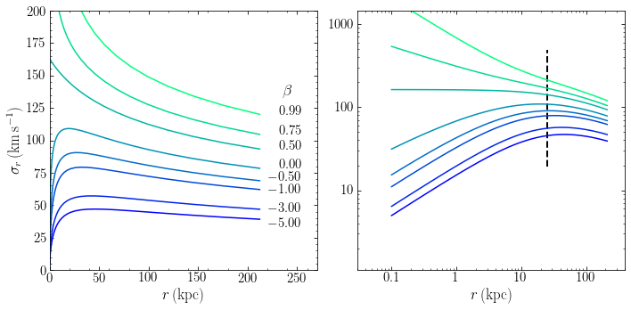
We show the radial velocity dispersion both on a linear scale as on a logarithmic scale so we can best study its behavior. We see that the velocity dispersion increases as we go from the virial radius inwards, but it only keeps increasing for \(\beta > 0.5\) and for such radially-anisotropic halos, the radial velocity dispersion increases without bounds. For \(\beta < 0.5\), the radial velocity dispersion decreases as one approaches the center. On the left, we indicate the scale radius of the profile by the dashed line, which shows that the transition between increasing and decreasing velocity dispersion occurs around the scale radius. The behavior of the velocity dispersion can be understood from solving the Jeans equation analytically in the regions \(r \ll a\) and \(r \gg a\). The overall scale of the radial velocity dispersion is higher for higher values of \(\beta\).
Using Equation \eqref{eq-anisotropy-2}, we can also compute the tangential dispersion \(\sigma_t = \sqrt{\sigma_\theta^2+\sigma_\phi^2}\) and this is displayed in the following figure:
[166]:
figsize(8,5)
for ii,beta in enumerate(betas):
    sigs= numpy.sqrt(2.*(1.-beta))\
        *numpy.array([jeans.sigmar(np,r,beta=beta).to_value(u.km/u.s) for r in rs])
    galpy_plot.plot(rs.to_value(u.kpc),
                    sigs,
                    semilogx=False,
                    xrange=[0.,290.],
                    yrange=[0.,180.],
                    gcf=True,
                    overplot=beta!=betas[0],
                    color=winter(ii/(len(betas)-1.)),
                    xlabel=r'$r\,(\mathrm{kpc})$',
                    ylabel=r'$\sigma_t\,(\mathrm{km\,s}^{-1})$')
plot(rs.to_value(u.kpc),np.vcirc(rs).to_value(u.km/u.s),'k--');
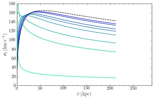
The magnitude of the tangential dispersion behaves opposite that of the radial velocity dispersion, increasing as \(\beta\) decreases, reflecting the increasing importance of tangential motions as \(\beta\) decreases. The dashed curve shows the rotation curve of the NFW profile for these parameters and we see that the tangential dispersion approaches the rotation curve as \(\beta \rightarrow -\infty\). Note that while we talk about “tangential dispersion” here and use the symbol \(\sigma_t\), what we actually calculate is \(\sqrt{\langle v_\theta^2\rangle + \langle v_\phi^2\rangle}\) and the tangential support can be provided either through dispersion or rotation. This makes it clear why the tangential dispersion approaches the circular velocity as \(\beta \rightarrow -\infty\): a purely-anisotropic, spherical system must have all bodies on circular orbits.
For more details on the solution of the spherical Jeans equation for NFW profiles, see Lokas & Mamon (2001).
6.5. The Jeans theorem
The Jeans equations are useful in using observational data to constrain the mass distribution of galaxies, but they suffer from the issue that they do not close in general and that solutions obtained under closure assumptions do not necessarily correspond to distribution functions that are everywhere positive: \(\forall \vec{x},\vec{v}: f(\vec{x},\vec{v}) \geq 0\). Therefore, we now move on to discussing full solutions \(f(\vec{x},\vec{v})\) of the equilibrium collisionless Boltzmann Equation \(\eqref{eq-collisionless-boltzmann-equil}\).
The Jeans theorem is an important theorem that significantly simplifies the problem of solving the equilibrium Boltzmann equation. It concerns integrals of motion, which we discussed in Chapter 5.3. From the definition of an integral of motion \(I(\vec{x},\vec{v})\) in Equation (5.63), we have that
If we write the derivative in terms of the partial derivatives with respect to \(\vec{x}\) and \(\vec{v}\), we find that
Comparing this to Equation \(\eqref{eq-collisionless-boltzmann-equil}\), we see that \(I(\vec{x},\vec{v})\) is a solution of the equilibrium collisionless Boltzmann equation. This immediately leads to the Jeans theorem:
Jeans theorem: Any function of the integrals of motion is a solution of the equilibrium collisionless Boltzmann equation. Furthermore, any solution of the equilibrium collisionless Boltzmann equation only depends on the phase-space coordinates \((\vec{x},\vec{v})\) through the integrals of motion.
Proof: Both statements directly follow from Equations \(\eqref{eq-const-integral-1}\) and \(\eqref{eq-const-integral}\): If \(f \equiv f(I_1,\ldots,I_n)\) is any function of \(n\) integrals of the motion, then \(\frac{\mathrm{d}f}{\mathrm{d} t} = \sum_i \frac{\partial f}{\partial I_i}\,\frac{\mathrm{d} I_i}{\mathrm{d} t} = 0\), by virtue of Equation \(\eqref{eq-const-integral-1}\). Conversely, if \(f(\vec{x},\vec{v})\) is a solution of the equilibrium collisionless Boltzmann equation, then Equation \(\eqref{eq-const-integral}\) holds for \(f(\vec{x},\vec{v})\) and therefore \(f(\vec{x},\vec{v})\) is an integral of the motion, straightforwardly satisfying the second part of the theorem.
The Jeans theorem implies that to find solutions of the equilibrium collisionless Boltzmann equations, we should constrain ourselves to looking for solutions that are functions of the integrals of the motion and that are positive for all \((\vec{x},\vec{v})\). For spherical systems, these integrals are \(E\) and \(\vec{L}\). Therefore, we only need to consider functions \(f \equiv f(E,\vec{L})\). If we are furthermore interested in self-consistent solutions where \(f\) sources the potential or in spherically-symmetric tracer distributions embedded in a spherical potential, the distribution function cannot depend on the orientation of the orbital plane (or the resulting [tracer] density distribution would not be spherically symmetric). Therefore, for spherical systems we generally only consider equilibrium distribution functions \(f \equiv f(E,L)\) (or also including the sign of \(L\) when considering rotation).
Before continuing, it is important to note that even though we will consider distribution functions of the form \(f(E,\vec{L})\), the distribution function is always considered to be a probability density on the phase-space coordinates. That is, \(f(\vec{x},\vec{v})\) has units of one over phase-space volume, because its integral over phase-space volume is a unitless number (the fraction of bodies in that phase-space volume). Therefore, even when we use a distribution function \(f \equiv f(E)\), as we do below, the distribution function still gives the probability of finding stars in a small volume around (\(\vec{x},\vec{v}\)): \(p(\vec{x},\vec{v}) = f(E[\vec{x},\vec{v}])\), not the probability of finding stars with energies in a small range around \(E\) (which would have units of one over energy, because its integral over an energy range would be a unitless number). Because canonical transformations preserve the phase-space volume element, it is well defined for any set of canonical coordinates \((\vec{q},\vec{p})\) to consider \(f(\vec{q},\vec{p})\) to represent the probability of finding stars in a small volume around \((\vec{q},\vec{p})\).
Seeking solutions of the collisionless Boltzmann equation through the Jeans theorem comes in general in two flavors: (i) finding self-consistent solutions that generate a given density profile (and potential) and (ii) finding solutions, which may or may not be self-consistent depending on the context, that are constrained by observational data. The first case is a purely theoretical problem—albeit one whose results might be applied to interpreting observational data—and we can search for the simplest distribution function that generates a given density profile. For the second case, we typically want to find the simplest solution that is consistent with the data (applying Occam’s razor) and this solution may be significantly more complicated.
6.6. Spherical distribution functions
Because of the simplicity of spherical systems, a large variety of spherical distribution functions \(f(E,L)\) have been studied in the literature. To find spherical distribution functions \(f(E,L)\) it is convenient to work with slightly different definitions of the potential, energy, and distribution function than we have used until now. We define the relative potential to be
for some constant \(\Phi_0\). We also define the relative energy \(\mathcal{E}\) as
where \(v = |\vec{v}|\). This is also a specific energy (that is, per unit mass), but we will simply refer to it as an “energy” in what follows. The constant \(\Phi_0\) will in general be chosen such that \(f > 0\) if \(\mathcal{E} > 0\) and \(f = 0\) when \(\mathcal{E} \leq 0\). For isolated systems with \(\Phi(\infty)=0\) that extend to \(\infty\), we can set \(\Phi_0 = 0\) and we simply have that \(\mathcal{E} = -E\), the binding energy. From the definition of the escape velocity in Equation (4.15), we then also have that
The Poisson equation in terms of the relative potential is
Furthermore, we will sometimes define the normalization of the distribution function to be such that \(\int \mathrm{d}\,\vec{x}\,\mathrm{d}\vec{v}\, f(\vec{x},\vec{v}) = M\), the total mass of the system rather than unity. Then we have that \(\rho(\vec{x}) = \int \mathrm{d} \vec{v}\,f(\vec{x},\vec{v})\), which can be useful in simplifying expressions.
6.6.1. Ergodic DFs and the Eddington inversion formula
The simplest solution of the collisionless Boltzmann equation for self-consistent systems is a distribution function that only depends on the (relative) energy, \(f \equiv f(\mathcal{E})\). Such distribution functions are called ergodic distribution functions. We will demonstrate that there is a unique ergodic distribution function for any spherical mass distribution \(\rho(r)\). However, this distribution function is not guaranteed to be everywhere non-negative and thus cannot necessarily be a physical solution when considered on its own. Not all spherical mass distributions can therefore be instantiated as ergodic distribution functions.
We start by writing the density \(\rho(r)\) in terms of the distribution function and changing variables from \(v\) to \(\mathcal{E}\) using Equation \(\eqref{eq-rel-energy}\)
where the second line follows because an isotropic distribution function only depends on the magnitude of the velocity and where the lower limit in the final line is zero because \(f = 0\) for \(\mathcal{E}\leq 0\). For any spherical potential, \(\Phi\)—and therefore also \(\Psi\)—is a monotonic function of radius (e.g., Equation 3.30), so we can write \(\rho\) as a function \(\rho(\Psi)\) of \(\Psi\) in a well-defined way and Equation \(\eqref{eq-to-eddington-1}\) can be written as
Differentiating with respect to \(\Psi\) gives
because the integrand is zero when \(\mathcal{E} = \Psi\). Equation \(\eqref{eq-to-eddington-3}\) is an Abel integral equation, which can be inverted to
or without the derivative of the integral
This is the Eddington formula (Eddington 1916). From Equation \(\eqref{eq-eddington-alt}\) it is clear that \(f(\mathcal{E})\) can only be everywhere non-negative if \(\int_0^\mathcal{E}\mathrm{d}\Psi\,\frac{1}{\sqrt{\mathcal{E}-\Psi}}\,\frac{\mathrm{d}\rho}{\mathrm{d}\Psi}\) is an increasing function of \(\mathcal{E}\). If this is not the case, then no ergodic distribution function is consistent with the density \(\rho(r)\). Because ergodic distribution functions only depend on the energy, which only depends on velocity through \(v^2 = v_r^2 + v_\theta^2+v_\phi^2\), such systems have \(\overline{\vec{v}} = 0\) and \(\overline{v_r^2} = \overline{v_\theta^2} = \overline{v_\phi^2}\), such that the anisotropy \(\beta = 0\) (see Equation \(\ref{eq-anisotropy}\)). This provides an example of a Jeans equation closure that would cause an unphysical situation: if we close the spherical Jeans equation by assuming \(\beta = 0\) for a density that does not satisfy the constraint that \(\int_0^\mathcal{E}\mathrm{d}\Psi\,\frac{1}{\sqrt{\mathcal{E}-\Psi}}\,\frac{\mathrm{d}\rho}{\mathrm{d}\Psi}\) must be an increasing function of \(\mathcal{E}\), then the solution found through the spherical Jeans Equation \(\eqref{eq-spher-jeans}\) would be unphysical.
We did not use the Poisson equation in the derivation of \(\eqref{eq-eddington}\). This equation therefore applies whether or not the density \(\rho\) that appears in it generates the potential or not. We also did not rely on the normalization of \(f\), so Equation \(\eqref{eq-eddington}\) applies no matter how we normalize \(f\).
To sample phase-space points from an ergodic distribution function, it is easiest to proceed as follows:
Sample \(r\) from the cumulative mass profile, e.g., using inverse transform sampling;
Sample random angles on the sphere \((\theta,\phi)\) (keeping in mind that while the distribution of \(\phi\) is uniform in \([0,2\pi]\), the distribution of \(\theta\) is \(p(\theta) \propto \sin\theta\) in \([0,\pi]\));
Sample the magnitude \(v\) of the velocity from \(p(v|r) \propto v^2 f(\mathcal{E}) = v^2 f(\Psi[r]-v^2/2)\). This can also be done using inverse transform sampling between \(v=0\) and the escape velocity \(v= v_\mathrm{esc}(r)\);
Sample velocity angles \((\eta,\psi)\) randomly on the sphere as well, to convert the magnitude of the velocity to the spherical velocity components as
\begin{align} v_r& = v\,\cos \eta\,,\\ v_\theta & = v\,\sin\eta\,\cos\psi\,,\\ v_\phi & = v\,\sin\eta\,\sin\psi\,. \end{align}By randomly distributing the magnitude of the velocity over radial and tangential components, an isotropic distribution function is obtained. Note that the tangential velocity \(v_t\) that is used for anisotropic distribution functions below is \(v_t = v\,\sin\eta\).
For the anisotropic distribution functions that we discuss below, the first three steps are the same (or very similar), but the final step will need to be adjusted to ensure the correct anisotropy of the distribution function.
Let’s use the Eddington formula to find a distribution function that self-consistently generates the Hernquist profile discussed in Section 3.4.6. The Hernquist profile has a mass \(M = 2\pi\,\rho_0\,a^3\) (see Equation 3.60) and a non-zero density at all \(r\). We therefore set \(\Phi_0 = 0\). Using the expression for the Hernquist potential from Equation (3.61), we can express \(r\) as a function of \(\Psi\) as
where
We can then express the Hernquist density from Equation (3.58) in terms of \(\Psi\) as (we use the number density \(\nu = \rho/M\) here rather than the mass density \(\rho\))
Taking the derivative of this with respect to \(\Psi\) and using the Eddington formula in the form from Equation \(\eqref{eq-eddington}\) gives the Hernquist distribution function
in terms of the dimensionless relative energy \(\tilde{\mathcal{E}} = \mathcal{E}\,a/(G\,M) = -E\,a/(G\,M)\).
One advantage of having a full equilibrium distribution-function for a given mass profile is that one can sample a realization of the distribution function as a set of bodies. These could then be used as the starting point of a numerical investigation, like an \(N\)-body simulation of the evolution of a merging satellite galaxy within a larger galaxy. As an example, we draw a realization of a Herquist mass profile that is similar to the dark-matter halo in the Milky Way (with a mass of \(M = 10^{12}\,M_\odot\) and a scale parameter \(a = 16\,\mathrm{kpc}\)). By binning the distribution of radial velocities \(v_r\) at different \(r\), we can compute the velocity dispersion of the sample of bodies and compare it to that obtained by solving the Jeans equation \eqref{eq-spher-jeans-anisotropy}:
[44]:
from galpy.potential import HernquistPotential
from galpy.df import isotropicHernquistdf
from galpy.df import jeans
from matplotlib.ticker import FuncFormatter
hp= HernquistPotential(amp=2.*1e12*u.Msun,a=16.*u.kpc)
dfh= isotropicHernquistdf(pot=hp)
orbs= dfh.sample(n=100000)
rs, vrs= orbs.r(), orbs.vr()
figsize(8,4)
subplot(1,2,1)
w,e= numpy.histogram(rs,range=[0.,40.],bins=31,weights=numpy.ones_like(rs))
mv2,_= numpy.histogram(rs,range=[0.,40.],bins=31,weights=vrs**2.)
brs= (numpy.roll(e,-1)+e)[:-1]/2.
plot(brs,numpy.sqrt(mv2/w),label=r'$\mathrm{samples}$')
# Compare to Jeans
plot(brs,numpy.array([jeans.sigmar(hp,r,beta=0.).to_value(u.km/u.s) for r in brs]),
     label=r'$\mathrm{Jeans\ eq.}$')
legend(frameon=False,fontsize=18.)
subplot(1,2,2)
w,e= numpy.histogram(numpy.log(rs.to(u.kpc).value),
                     range=[numpy.log(1),numpy.log(100.)],
                     bins=31,weights=numpy.ones_like(rs))
mv2,_= numpy.histogram(numpy.log(rs.to(u.kpc).value),
                       range=[numpy.log(1),numpy.log(100.)],
                       bins=31,weights=vrs**2.)
brs= numpy.exp((numpy.roll(e,-1)+e)[:-1]/2.).to_value(u.dimensionless_unscaled)
semilogx(brs,numpy.sqrt(mv2/w),label=r'$\mathrm{samples}$')
# Compare to Jeans
semilogx(brs,numpy.array([jeans.sigmar(hp,r*u.kpc,beta=0.).to_value(u.km/u.s)
                          for r in brs]),
        label=r'$\mathrm{Jeans\ eq.}$')
legend(frameon=False,fontsize=18.)
subplot(1,2,1)
xlabel(r'$r\,(\mathrm{kpc})$')
ylabel(r'$\sigma_r\,(\mathrm{km\,s}^{-1})$')
subplot(1,2,2)
xlabel(r'$r\,(\mathrm{kpc})$')
gca().xaxis.set_major_formatter(FuncFormatter(
                lambda y,pos: (r'${{:.{:1d}f}}$'.format(int(\
                    numpy.maximum(-numpy.log10(y),0)))).format(y)))
tight_layout();
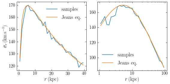
To better show the radial behavior, we have binned the bodies both in equal-width bins in radius \(r\) and in \(\log r\). We see that the velocity dispersion of the sample of bodies matches that computed using the Jeans equation very well. But the full distribution function also allows us to go beyond just a simple velocity dispersion and look at, for example, the distribution of radial velocities at different radii. As an example of that, we plot the distribution of the magnitude \(v\) of the velocity, \(p(v|r) = v^2 f(\mathcal{E}[r,v])\), at three different radii:
[42]:
figsize(6,4)
rs= [1.*u.kpc,8.*u.kpc,32.*u.kpc]
for r in rs:
    vs= numpy.linspace(0.,hp.vesc(r),101)
    # p(v|r) ~ v^2 f(E[r,v])
    pvr= vs**2.*dfh(r,vs,0.,0.,0.).to_value(1./(u.kpc*u.km/u.s)**3)
    pvr/= numpy.sum(pvr*(vs[1]-vs[0]))
    plot(vs,pvr,label=r'$r = {:.0f}\,\mathrm{{kpc}}$'.format(r.to_value(u.kpc)))
xlabel(r'$v\,(\mathrm{km\,s}^{-1})$')
ylabel(r'$p(v|r)$')
legend(frameon=False,fontsize=18.);
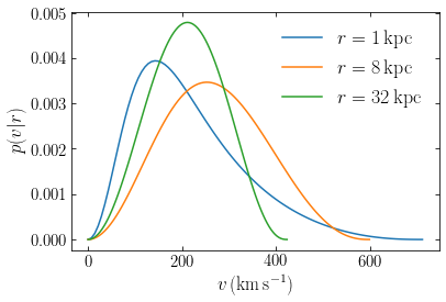
The distributions are shown up to the escape velocity at the different radii and you can see the diminishing escape velocity diminishes increasing radius as the decrease of the extent of the velocity distribution. The width of the velocity distribution is largest for the intermediate radius (being at \(r=8\) kpc in our Milky-Way-inspired model, this is a proxy for the dark-matter velocity distribution near the Sun), as expected from the Jeans equation (see the figure above). But the shape of the velocity distribution changes non-trivially with radius and only a full distribution-function model of a dynamical system can provide this full distribution.
6.6.2. The isothermal sphere
A different approach to solving the collisionless Boltzmann equation using the Jeans theorem is to posit a form for \(f(\mathcal{E},L)\)—for a spherical system—and determine what density profile it corresponds to. In this case you do not know what will come out, but what you get might be useful! This procedure can be followed for self-consistent and non-self-consistent distribution functions: in the former case, we need to use the constraint that the density \(\rho(r) = \int \mathrm{d}v\,v^2\,f(\mathcal{E},L)\) sources the potential through the Poisson equation, in the latter case one simply computes the energy using an external potential.
Let’s consider a distribution function \(f(\mathcal{E})\) of the following form
with parameters \((\rho_1,\sigma)\). Unlike most of the distribution functions that we discuss in this chapter, this distribution function extends all the way down to \(\mathcal{E} = -\infty\) (we will see below that this is because this system has infinite mass and therefore all orbits are bound). Because \(\Psi\) only depends on \(r\), the velocity distribution at any given \(r\) is a Gaussian and the density obtained by integrating over all velocities is (see Equation \ref{eq-to-eddington-1-int})
For a self-consistent system, a second relation between \(\rho(r)\) and \(\Psi\) comes from the Poisson equation (in terms of \(\Psi\): Equation \([\ref{eq-poisson-psi}]\)) for a spherical system
Substituting Equation \(\eqref{eq-isothermaldf-dens-derivation}\) in the Poisson equation gives
One solution of this equation is
which is the singular isothermal sphere. This solution is “singular”, because it diverges as \(r \rightarrow 0\). It is isothermal, because the velocity distribution—the conditional probability distribution \(p(v|r)\) of velocity at a given radius \(r\)—at any radius is a spherical Gaussian with dispersion \(\sigma\), which can be seen directly from Equation \(\eqref{eq-isothermal-df-form}\):
From Equation \(\eqref{eq-isothermaldf-dens-derivation}\), we find the potential
and the circular velocity \(v_c(r)\) is
The singular isothermal sphere therefore corresponds to the distribution function of a spherical distribution of matter that gives rise to a flat rotation curve. For this reason, the isothermal sphere is an important distribution-function model. This correspondence also demonstrates the success of the second approach to solving the collisionless Boltzmann equation. Simply by positing a simple form for the distribution function (Equation \([\ref{eq-isothermal-df-form}]\)) we found an important self-consistent, approximate model for galaxies with a flat rotation curve!
6.6.3. Distribution functions for globular clusters: King profiles
Despite its simplicity, the isothermal sphere model above has significant issues if we want to use it to model real stellar systems. Primary among these is the fact that it has infinite mass and to model a real system we therefore have to cut it off in some manner. A simple way of achieving this is to modify Equation \(\eqref{eq-isothermal-df-form}\) to
for \(\mathcal{E} > 0\) and zero otherwise. This family of models is known as King models and they are a popular model for globular clusters (Michie 1963; Michie & Bodenheimer 1963; King 1966). Integrating over velocity gives the density as a function of \(\Psi\)
where we have defined \(\tilde{\Psi} = \Psi/\sigma^2\). The Poisson equation then becomes
This equation needs to be solved numerically, which we can do by starting at \(r=0\), assuming \(\mathrm{d}\Psi / \mathrm{d} r = 0\) and starting from some chosen value of \(\Psi(0)\). Equation \(\eqref{eq-king-poisson}\) is then an ordinary differential equation that can be solved to give \(\Psi(r)\). As we have already discussed, \(\Psi(r)\) decreases as \(r\) increases for any spherical potential and therefore at some \(r = r_t\) we have that \(\Psi(r_t) = 0\). From Equation \(\eqref{eq-king-dens-implicit}\) it is clear that \(\rho = 0\) when \(\Psi =0\) and therefore the density becomes zero at \(r_t\) (it remains zero for \(r > r_t\), because we have that \(f(\mathcal{E}) = 0\) for \(\mathcal{E} \leq 0\) and \(\mathcal{E} \leq 0\) when \(\Psi < 0\)). The radius \(r_t\) is the tidal radius. Once we have found the tidal radius, we can determine the central potential \(\Phi(0)\), because from Newton’s second theorem discussed in Section 3.2 we know that \(\Phi(r_t) = -G\,M/r_t\), where \(M = 4\pi\,\int \mathrm{d}r\,r^2\rho(r)\) is the total mass of the system: \(\Phi(0) = \Phi(r_t) - \Psi(0)\) from Equation \(\eqref{eq-psi-phi}\).
Besides the tidal radius, another typical radius for a King model is the King radius \(r_0\) defined as
where \(\rho_0\) is the (finite) central density obtained from Equation \(\eqref{eq-king-dens-implicit}\). The ratio of the tidal to the King radius gives the concentration, technically defined as
King models form a three-dimensional sequence of mass, tidal radius, and concentration. The latter is also often parameterized in terms of \(W_0 = \Psi(0)/\sigma^2\), because this allows the King model for a given mass, tidal radius, and \(\Psi(0)/\sigma^2\) to be straightforwardly computed using the procedure described above. In fact, if you inspect the equations above carefully, you see that the fundamental structure of the model, \(\Psi(r)\) and \(\mathrm{d}\Psi(r) / \mathrm{d}r\), can be computed by working in the scaled parameter \(W = \Psi/\sigma^2\). The obtained solution \((W[r],\mathrm{d} W/\mathrm{d}r)\) can then used with any desired mass and tidal radius by simply scaling the mass and tidal radius to the desired values.
To get a sense of what these King models look like, let’s compute the density profile for a range of values of the scaled central potential \(W_0\). Because the mass (or density) and length scales are unimportant for the overall shape of the distribution, we plot the radius as a fraction of \(r_0\) and the density as a fraction of the central density \(\rho_0\):
[90]:
from galpy.df import kingdf
from matplotlib.ticker import FuncFormatter
W0s= [1.,3.,5.,7.,9.,11]
figsize(7,5)
for W0 in W0s:
    dfk= kingdf(W0=W0)
    conc= numpy.log10(dfk.rt/dfk.r0)
    rs= numpy.geomspace(dfk.r0/100.,dfk.rt,101)
    loglog(rs/dfk.r0,dfk.dens(rs)/dfk.rho0,label=r'${:.0f}$'.format(W0))
xlim(3e-2,3e2)
ylim(1e-6,2)
xlabel(r'$r/r_0$')
ylabel(r'$\rho(r)/\rho_0$')
gca().xaxis.set_major_formatter(FuncFormatter(
                lambda y,pos: (r'${{:.{:1d}f}}$'.format(int(\
                    numpy.maximum(-numpy.log10(y),0)))).format(y)))
text(8e-2,2e-2,r'$W_0$',fontsize=18.,horizontalalignment='center')
legend(frameon=False,fontsize=18.,loc='lower left');
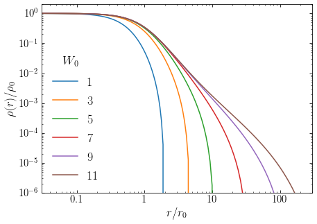
We see that for small values of \(W_0\), the King model is essentially a homogeneous-density sphere that is cut off at the tidal radius. At large values of \(W_0\), there is a small core and outside of the core the density drops as \(\rho(r) \approx r^{-2}\) until the tidal radius is reached.
From the definition of the King distribution function in Equation \(\eqref{eq-king-df-form}\) it is clear that at large binding energies \(\mathcal{E} \gg 0\) the distribution function is approximately that of the isothermal sphere and the velocity distribution is therefore a spherical Gaussian with dispersion \(\sigma\). As \(r\) increases, \(\mathcal{E} \rightarrow 0\) and the velocity dispersion approaches zero. We can see this behavior if we compute the velocity dispersion as a function of radius for the models shown above
[99]:
from galpy.df import kingdf
from matplotlib.ticker import FuncFormatter
W0s= [1.,3.,5.,7.,9.,11]
figsize(7.5,5)
for W0 in W0s:
    dfk= kingdf(W0=W0)
    conc= numpy.log10(dfk.rt/dfk.r0)
    # Approach rt logarithmically, to better resolve the behavior there
    rs= numpy.hstack((numpy.geomspace(dfk.r0/100.,numpy.amax([dfk.r0,dfk.rt/10.]),101),
                      sorted(dfk.rt-numpy.geomspace(1e-4,dfk.rt-numpy.amax([dfk.r0,dfk.rt/10.]),101))))
    semilogx(rs/dfk.r0,numpy.array([dfk.sigmar(r) for r in rs])
               /dfk.sigma,label=r'${:.0f}$'.format(W0))
xlim(3e-2,3e3)
ylim(0.,1.1)
xlabel(r'$r/r_0$')
ylabel(r'$\sigma(r)/\sigma$')
gca().xaxis.set_major_formatter(FuncFormatter(
                lambda y,pos: (r'${{:.{:1d}f}}$'.format(int(\
                    numpy.maximum(-numpy.log10(y),0)))).format(y)))
text(600,1.,r'$W_0$',fontsize=18.,horizontalalignment='center')
legend(frameon=False,fontsize=18.,loc='upper right',bbox_to_anchor=(1,0.92));
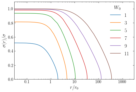
We have normalized the velocity dispersion by the parameter \(\sigma\) and the figure above makes clear that this parameter \(\sigma\) is not the actual velocity dispersion of the model anywhere (except for large \(W_0\), where the core dispersion is approximately \(\sigma\), because the distribution function is very close to isothermal there).
Because the King model is an ergodic distribution function, the velocity anisotropy is zero. A generalization of the King models that have non-zero anisotropy is given by the Michie models (Michie & Bodenheimer 1963).
6.6.4. Anisotropic distribution functions
So far we have only considered ergodic distribution functions, which are always isotropic because the velocities enter the specific energy \(E\) only through \(v^2 = v_r^2 + v_\theta^2+v_\phi^2\) and the velocity dispersion in different directions therefore have to equal each other. However, realistic stellar systems often have some degree of anisotropy. Dark matter halos in the standard cold-dark-matter paradigm are close to isotropic only near their centers, becoming radially biased in their outskirts (\(\beta \approx 0.5\); Diemand et al. 2004; Wojtak et al. 2005). Stars in globular clusters and stellar halos can also have non-isotropic velocity distributions that are not well captured by ergodic distribution functions. To investigate such systems in more detail, we, therefore, require a way to create anistropic distribution function models.
We will only consider anisotropic distribution functions for spherical, non-rotating systems. Such distribution functions can only depend on the magnitude \(L = |\vec{L}|\) of the specific angular momentum in addition to the specific energy \(E\), so we will consider functions \(f(E,L)\). As before, distribution functions are most easily expressed in terms of the relative energy \(\mathcal{E}\) defined in Equation \eqref{eq-rel-energy} and we will therefore consider the function \(f(\mathcal{E},L)\). As for ergodic distribution functions, one important model-building task is to find an anisotropic distribution function \(f(\mathcal{E},L)\) that generates a given density profile \(\rho(r)\). The equation relating the distribution function and the density that is analogous to Equation \eqref{eq-to-eddington-1} for the ergodic case is now
where \(v_t = \sqrt{v_\theta^2+v_\phi^2}\) and as in the ergodic case we require knowledge of \(\Psi(r)\). Unlike Equation \eqref{eq-to-eddington-1}, Equation \eqref{eq-dens-anisotropic-general-1} cannot be directly inverted, mathematically, because a function of a single variable, \(\rho(r)\), is not sufficient to determine a function of two variables, \(f(\mathcal{E},L)\). Physically what happens is that, once we allow for any anisotropy profile, many distribution functions are consistent with the same spatial density.
To make progress in inverting Equation \eqref{eq-dens-anisotropic-general-1}, we therefore need to constrain the possible solutions. This could be done by positing specific forms for \(f(\mathcal{E},L)\) and solving the inversion, but this has the disadvantage of appearing quite ad hoc. Because our first inkling of the breaking of the ergodic assumption typically comes from measurements of the orbital anisotropy \(\beta(r)\), we would like a procedure that guides us towards solutions with a given anisotropy profile. One way to do this, is to consider the density defined by the right-hand side of Equation \eqref{eq-dens-anisotropic-general-1} as a function not just of \(r\), but as a two-dimensional function of \((\Psi,r)\) called the augmented density (Dejonghe 1986)
The true density is obtained as \(\rho(r) = \tilde{\rho}(\Psi[r],r)\). We can then create unique anisotropic distribution functions for a given density \(\rho(r)\), by positing a form for \(\tilde{\rho}(\Psi,r)\) that satisfies \(\rho(r) = \tilde{\rho}(\Psi[r],r)\); because \(\tilde{\rho}(\Psi,r)\) is a function of two variables, it can uniquely determine \(f(\mathcal{E},L)\) and, in fact, one can show that it does (Dejonghe 1986).
To gain insight into the meaning of the augmented density, we can compute the radial and tangential velocity dispersions, \(\sigma_r\) and \(\sigma_t\). We have that
and thus using Equation \eqref{eq-dens-anisotropic-general-2}
or
Similarly, for the tangential velocity dispersion \(\sigma_t\), we have that
To relate this to the augmented density, we first re-write Equation \eqref{eq-dens-anisotropic-general-2} as
We can then see that
and thus
Therefore, we can easily compute the radial and tangential velocity dispersions given the augmented density using Equations \eqref{eq-anidf-sigr-aug} and \eqref{eq-anidf-sigt-aug}. The orbital anisotropy then directly follows from its definition
Thus, we see that the augmented density is directly related to a model’s anisotropy profile. As one would expect from the Eddington-inversion argument, an augmented density that is a function of the potential alone, \(\tilde{\rho}(\Psi,r) \equiv \rho(\Psi)\), corresponds to an isotropic distribution function and the inversion equation \eqref{eq-dens-anisotropic-general-2} reduces to the Eddington inversion.
Unfortunately, inverting Equation \eqref{eq-dens-anisotropic-general-2} for a general augmented density is difficult (requiring combined forward and inverse Laplace and Mellin transformations; Dejonghe 1986). However, we can make progress by considering augmented densities that are separable functions of \(\Psi\) and \(r\):
Then the anisotropy from Equation \eqref{eq-anidf-beta-aug} reduces to the simpler expression
6.6.4.1. Distribution functions with constant anisotropy
Armed with Equation \eqref{eq-anidf-beta-aug-sep}, we can now proceed to construct distribution functions that have constant anisotropy as a function of radius. Substituting \(g(r) = r^{-2\beta}\) into Equation \eqref{eq-anidf-beta-aug-sep}, we find that \(\beta(r) = \beta\) constant with radius, and therefore models with constant anisotropy can be obtained using the augmented density
Because \(r\) only enters the relation \eqref{eq-dens-anisotropic-general-2} between \(\tilde{\rho}(\Psi,r)\) and \(f(\mathcal{E},L)\) through \(f(\mathcal{E},L)\) itself, it is clear that this augmented density must correspond to a distribution function
where
The inner integral can be worked out and using Equation \eqref{eq-anidf-constbeta-aug} to write \(f_\Psi(\Psi)\) in terms of the density, we get
Before discussing the general solution of this inversion, it is worth noting that the case \(\beta = 1/2\) is especially simple, because then Equation \eqref{eq-anidf-constbeta-inveq-1} simplifies to
and therefore
As an example, for the Hernquist profile, combining Equations \eqref{eq-spherdf-hernquist-r-psi} and \eqref{eq-spherdf-hernquist-dens-psi}, we have that
where \(\tilde{\Psi} = \Psi a/[GM]\). Therefore, a distribution function with constant anisotropy \(\beta = 1/2\) for the Hernquist profile is given by
In fact, all half-integer values of \(\beta\) are of a similar simplicity, because we can take a suitable number of derivatives of Equation \eqref{eq-anidf-constbeta-inveq-1} with respect to \(\Psi\) to make the exponent of \((\Psi-\mathcal{E})\) in the integrand equal to zero. For example, for \(\beta = -1/2\), we first take the derivative of Equation \eqref{eq-anidf-constbeta-inveq-1} with respect to \(\Psi\) to get
and then plugging in \(\beta = -1/2\), we find that
or
In this case, for the Hernquist profile, we have that
where again \(\tilde{\Psi} = \Psi a/[GM]\), and therefore
where \(\tilde{\mathcal{E}} = \mathcal{E} a/[GM]\).
For general, half-integer \(\beta\) solution we need to take \(1/2-\beta\) derivatives of Equation \eqref{eq-anidf-constbeta-inveq-1} with respect to \(\Psi\) to make the exponent of \((\Psi-\mathcal{E})\) equal to zero and then another derivative to remove the integral. Thus, we generate a factor \(\Gamma(3/2-\beta)\) from \(\mathrm{d}^{1/2-\beta} (\Psi-\mathcal{E})^{1/2-\beta} / \mathrm{d} \Psi^{1/2-\beta}\) that exactly cancels the same factor in the denominator in Equation \eqref{eq-anidf-constbeta-inveq-1} and the remaining pre-factors can succinctly written in terms of the double factorial \((-2\beta)!! = 2^{1/2-\beta}\,\Gamma(1-\beta)/\sqrt{\pi}\), leading to (Cuddeford 1991; An & Evans 2006)
For non-half-integer values of \(\beta\), we can solve for \(f_\mathcal{E}(\mathcal{E})\) by noting that Equation \eqref{eq-anidf-constbeta-inveq-1} is an Abel integral equation similar to Equation \eqref{eq-to-eddington-3} for a similar suitable number of derivatives of the equation with respect to \(\beta\) (the number of derivatives required is that to make the exponent of \((\Psi-\mathcal{E})\) in the integrand between \(0\) and \(-1\)); the full solution of this Abel inversion is given by
where \(m = \lfloor 3/2-\beta \rfloor\) and \(\alpha = 3/2-\beta-m\).
While this isn’t an easy integral to solve, for values of \(\beta\) that are not too far from zero, computing this integral is not that much more onerous than evaluating the equivalent integral for the isotropic case (Equation \ref{eq-eddington}). The main bottleneck is computing the derivatives of the density times \(r^{2\beta}\) with respect to \(\Psi\). Sampling from these constant-anisotropy distribution functions proceeds in the same way as for ergodic distribution functions as described in Section 6.6.1, except that the velocity angle \(\eta\) is now sampled from \(p(\eta) \propto \sin^{1-2\beta}\eta\) (because of the \(L^{-2\beta} = r^{-2\beta}\,v_t^{-2\beta} = r^{-2\beta}\,v^{-2\beta}\,\sin^{-2\beta}\eta\) additional factor in the distribution function compared to the ergodic case). This can be sampled using inverse transform sampling and the cumulative distribution can be worked out in terms of a hypergeometric function (but it cannot be analytically inverted, so it needs to be inverted using interpolation).
For the Hernquist profile, the integral in Equation \eqref{eq-anidf-constbeta-generalsol} can be performed analytically for all \(\beta\) and expressed as (Baes & Dejonghe 2002)
where \({}_2 F_1\) is the hypergeometric function and, as usual for the Hernquist profile, \(\tilde{\mathcal{E}} = \mathcal{E} a/[GM]\).
As an example, we can look at the distribution of total velocities \(v^2 = v_r^2+v_t^2\) at a given radius in Hernquist profiles with different constant anisotropy parameters. Making use of the fact that a full distribution function model allows us to sample points from the distribution function, let’s do this by sampling points at the given radius. We’ll look at \(r = 8\,\mathrm{kpc}\) in the same Milky-Way dark-matter-halo-like Hernquist profile as in Section 6.6.1 above:
[12]:
from galpy.potential import HernquistPotential
from galpy.df import constantbetaHernquistdf
hp= HernquistPotential(amp=2.*1e12*u.Msun,a=16.*u.kpc)
betas= [0.5,0,-0.5,-1.5]
r= 8.*u.kpc
for beta in betas:
    dfh= constantbetaHernquistdf(pot=hp,beta=beta)
    orbs= dfh.sample(R=r,z=0.,n=100000)
    vs= numpy.sqrt(orbs.vR()**2.+orbs.vT()**2.+orbs.vz()**2.)
    w,e= numpy.histogram(vs.to_value(u.km/u.s),bins=61,
                         range=[0.,hp.vesc(r).to_value(u.km/u.s)])
    plotvs= (numpy.roll(e,1)+e)[1:]/2.
    plot(plotvs,w/numpy.sum(w)/(plotvs[1]-plotvs[0]),
         label=r'$\beta = {:+.1f}$'.format(beta))
xlabel(r'$v\,(\mathrm{km\,s}^{-1})$')
ylabel(r'$p(v|r)$')
legend(frameon=False,fontsize=18.);
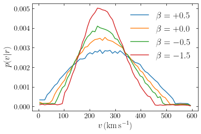
We see that as \(\beta\) decreases, the distribution of velocities narrows and the entire shape changes from a wide distribution at positive \(\beta\) to a more Gaussian-like distribution at tangential values of \(\beta\). As \(\beta\) decreases and the distribution of velocities becomes more and more tangential, eventually all orbits become circular and this distribution narrows to a delta function centered on the circular velocity (note that in practice, the hypergeometric functions become so large that numerically it is difficult to go to \(\beta \lesssim -30\)):
[11]:
hp= HernquistPotential(amp=2.*1e12*u.Msun,a=16.*u.kpc)
betas= [-1.5,-10.5,-30.5]
r= 8.*u.kpc
for beta in betas:
    dfh= constantbetaHernquistdf(pot=hp,beta=beta)
    orbs= dfh.sample(R=r,z=0.,n=100000)
    vs= numpy.sqrt(orbs.vR()**2.+orbs.vT()**2.+orbs.vz()**2.)
    w,e= numpy.histogram(vs.to_value(u.km/u.s),bins=61,
                         range=[0.,hp.vesc(r).to_value(u.km/u.s)])
    plotvs= (numpy.roll(e,1)+e)[1:]/2.
    plot(plotvs,w/numpy.sum(w)/(plotvs[1]-plotvs[0]),
         label=r'$\beta = {:+.1f}$'.format(beta))
axvline(hp.vcirc(r).to_value(u.km/u.s),color='k',ls='--',zorder=0,
       label=r'$v_c(r)$')
xlabel(r'$v\,(\mathrm{km\,s}^{-1})$')
ylabel(r'$p(v|r)$')
legend(frameon=False,fontsize=18.);
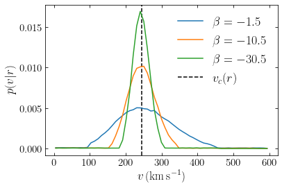
As for ergodic distribution functions obtained using the Eddington inversion, there is no guarantee that the constant-anisotropy distribution functions computed using this method are positive everywhere and this needs to be checked before proceeding with using these distribution functions. For example, the anisotropic Hernquist distribution functions derived here have negative density regions whenever \(\beta > 1/2\).
6.6.4.2. Distribution functions with radially-varying anisotropy
The orbital distribution of many galactic systems does not have constant anisotropy everywhere, but instead varies with radius. For example, as we already discussed above, dark matter halos in the standard cold-dark-matter paradigm are close to isotropic near the centers, but they become radially biased in their outskirts, with typical values of \(\beta \approx 0.3\) to \(0.7\). To model such systems, we require distribution function models with radially-varying anisotropy for a given density profile. Equation \eqref{eq-anidf-beta-aug-sep} in principle provides a way to do this for a given \(\beta(r)\) profile: solve this differential equation for \(g(r)\) that gives rise to a given \(\beta(r)\) profile, use it to define the augmented density from the density using Equation \eqref{eq-anidf-aug-sep}, and then invert Equation \eqref{eq-dens-anisotropic-general-2} to obtain \(f(\mathcal{E},L)\). However, the inversion in the last step does not have a clean solution for most \(\beta(r)\) profiles.
For certain \(\beta(r)\) profiles, the inversion of Equation \eqref{eq-dens-anisotropic-general-2} can be done more easily and a particularly elegant solution is possible for the anisotropy profile (Osipkov 1979; Merritt 1985)
Such an anisotropy profile results from a distribution function, known as an Osipkov-Merritt distribution function, that is a function of
alone, that is \(f \equiv f(Q)\). Before demonstrating that, let us take a look at how \(Q\) behaves as a function of \(\mathcal{E}\) and \(L\) for a given \(r_a\); we will use that to set an additional constraint on the distribution function. Bound orbits populate the region between \(L = 0\) and \(L = L_c(\mathcal{E})\), that is, between radial orbits and circular orbits of a given energy; we plot this as the hatched region below. For a Hernquist potential (using the usual normalized energy \(\tilde{\mathcal{E}} = \mathcal{E}\,a/[GM]\)) and using \(r_a = a/2\), we find the following behavior of \(\tilde{Q} = Q\,a/[GM]\):
[148]:
from galpy.potential import HernquistPotential
a=16.*u.kpc
ra= a/2
hp= HernquistPotential(amp=2.*1e12*u.Msun,a=a)
Es= numpy.linspace(0.,-0.99,1001)
def Lc(E):
    # Return the angular momentum of a circular orbit
    # with energy E
    rE= numpy.amax(numpy.roots([-E,2*-E-0.5,-E-1])*a)
    return rE*hp.vcirc(rE)
plot(Es,[Lc(E)/Lc(-0.5) for E in Es],color='k')
fill_between(Es,[Lc(E)/Lc(-0.5) for E in Es],hatch='/',fc='w')
xlabel(r'$-\tilde{\mathcal{E}}$')
ylabel(r'$L/L_c(\tilde{\mathcal{E}} = 1/2)$')
xs= numpy.linspace(-2.25,1.5,1001)*(-hp(0,0))
ys= numpy.geomspace(0.003,100,101)*Lc(-0.5)
xv, yv = numpy.meshgrid(xs,ys,indexing='ij')
Qv= -xv-yv**2./2./(ra)**2.
C= contour(xv/(-hp(0,0)),yv/Lc(-0.5),Qv/(-hp(0,0)),
           levels=[-3,-2,-1,-0.5,0.,0.5,0.9])
gca().clabel(C,inline=1,fontsize=14)
ylim(0.,4);
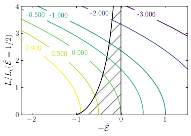
As expected, curves of constant \(Q\) (the labeled contours) are parabolas that curve leftwards for the axes used in this figure. The region to the left of the hatched region is not populated by any orbit in the potential, whether bound or unbound, because it consists of combinations of the energy and angular momentum that cannot be attained for any phase-space point (there are no energies less than that of the most bound orbit and there are no angular momenta larger than the circular one at a given energy). We can therefore ignore this region. However, the region to the right of the hatched region consists of unbound orbits and could therefore be populated. But such orbits cannot be used to build an equilibrium model and we should therefore not include them in such a model. As can be seen, these orbits all have \(Q < 0\). Orbits with \(Q < 0\) do exist within the bound, hatched region, but we choose to exclude these as well to simplify the resulting distribution function. We could keep them, but then we would have to carefully make sure to exclude all unbound orbits when working with the distribution function. Therefore, we additionally impose that \(Q \geq 0\).
Before computing the anisotropy, we can first get a sense of what type of anisotropy behavior to expect. When \(r_a\) is so large that \(\mathcal{E} >> L^2/[2r_a^2]\), it is clear that \(f(Q)\) becomes approximately \(f(\mathcal{E})\), that is, an isotropic, ergodic distribution function. The opposite extreme, where \(r_a\) is very small, is less straightforward, but we can understand what happens by looking at the contours of \(Q\) when \(r_a\) is small. Therefore, we plot similar contours of \(\tilde{Q}\) as in the example above, but now for \(r_a = a/20\):
[149]:
a=16.*u.kpc
ra= a/20
hp= HernquistPotential(amp=2.*1e12*u.Msun,a=a)
Es= numpy.linspace(0.,-0.99,1001)
plot(Es,[Lc(E)/Lc(-0.5) for E in Es],color='k')
fill_between(Es,[Lc(E)/Lc(-0.5) for E in Es],hatch='/',fc='w')
xlabel(r'$-\tilde{\mathcal{E}}$')
ylabel(r'$L/L_c(\tilde{\mathcal{E}} = 1/2)$')
xs= numpy.linspace(-2.25,1.5,1001)*(-hp(0,0))
ys= numpy.geomspace(0.003,100,101)*Lc(-0.5)
xv, yv = numpy.meshgrid(xs,ys,indexing='ij')
Qv= -xv-yv**2./2./(ra)**2.
C= contour(xv/(-hp(0,0)),yv/Lc(-0.5),Qv/(-hp(0,0)),
           levels=[-3.5,-2.5,-1.5,-0.5,0.,0.5,0.9])
gca().clabel(C,inline=1,fontsize=14)
ylim(0.,0.55);
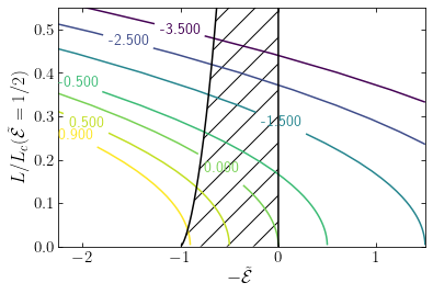
Because \(r_a\) is small, the \(L^2/[2r_a^2]\) terms is large and the contours therefore become more horizontal. Because we are only considering \(Q \geq 0\) to build the distribution function, allowed values of \(L\)—which are located in the intersection between the hatched region and the \(Q \geq 0\) region—are much smaller than before. The model therefore largely consists of radial orbits and as \(r_a\) decreases, the orbit becomes more and more radial until it eventually becomes purely radial as \(r_a \rightarrow 0\). Therefore, we can expect the form \(f(\mathcal{E}-L^2/[2r_a^2])\) to give rise to an anisotropy profile that is isotropic at \(r \ll r_a\) and fully radially anisotropic at \(r \gg r_a\) with a smooth transition between these regimes around \(r \approx r_a\).
To compute the actual anisotropy profile and work out how to obtain \(f(Q)\) for a given density profile, we obtain the augmented density using Equation \eqref{eq-dens-anisotropic-general-2}. We first interchange the order of the integrals in the general expression to give
and then we substitute the form \(f(Q)\) for \(f(\mathcal{E},r\,v_t)\)
Re-writing the inner integral in terms of \(Q\) then given
where we have used the constraint that \(f(Q)\) is only non-zero for \(Q \geq 0\). We then write the outer integral in terms of \(\tilde{v}^2_t = v_t^2\,\left(1+[r/r_a]^2\right)\) and also interchange the order of the integration once more
This inner integral can now be computed to give
Thus, the augmented density is of the separable form of Equation \eqref{eq-anidf-aug-sep} with \(g(r) = 1/(1+r^2/r_a^2)\) and
From \(g(r)\) and Equation \eqref{eq-anidf-beta-aug-sep}, we find that the anisotropy profile is
This profile has the behavior that we expected, with \(\beta \approx 0\) for \(r \ll r_a\) and \(\beta \approx 1\) for \(r \gg r_a\). The full behavior looks as follows:
[153]:
rs= numpy.linspace(0.,5.,101)
plot(rs,1./(1+1./rs))
xlabel(r'$r/r_a$')
ylabel(r'$\beta$');
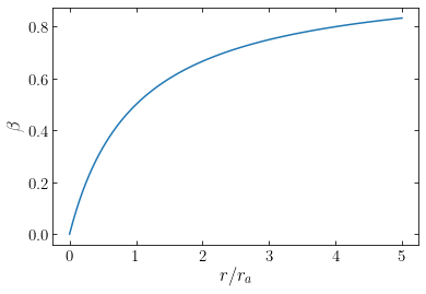
The anisotropy rises quickly to \(\beta = 1/2\) at \(r = r_a\) and then slowly approaches \(\beta = 1\). Nevertheless, this anisotropy profile is a reasonable, simple model for an anisotropic dark-matter halo if we set \(r_a \approx r_\mathrm{vir}\) to have \(\beta \approx 0.5\) at the virial radius \(r_\mathrm{vir}\).
To compute the distribution function \(f(Q)\) for a given spherical density profile \(\rho(r)\), we need to invert Equation \eqref{eq-anidf-osipkov-fpsi}. Comparing this equation to Equation \eqref{eq-to-eddington-2} that we encountered in deriving the Eddington inversion for ergodic distribution functions, we see that these equations are the same if we replace \(\rho(\Psi)\) in Equation \eqref{eq-to-eddington-2} with \(f_\Psi(\Psi) = \rho(\Psi)/g(r[\Psi]) = \rho(\Psi)\,(1+r^2[\Psi]/r_a^2)\). A similar Abel inversion therefore leads to
(an expression similar to Equation \ref{eq-eddington-alt} can also be derived). Obtaining the Osipkov-Merritt distribution function for a given density profile is therefore very similar to computing the ergodic distribution function with the only difference being that the density \(\rho(r)\) in the calculation is replaced by \(\rho(r)\,(1+r^2/r_a^2)\), but everything else being exactly the same. Because the density only enters as \(\rho(r)\,(1+r^2/r_a^2)\), the calculation can actually be split into a part that is identical to the Eddington formula and a part proportional to \(r_a^{-2}\) as
where \(f^{\beta=0}(Q)\) is the ergodic distribution function computed using the Eddington formula \eqref{eq-eddington}.
Sampling from Osipkov-Merritt-type distribution functions proceeds along the same lines as for ergodic distribution functions as described in Section 6.6.1, sampling positions \((r,\theta,\phi)\) in the same way. But now we need to first sample the velocity angle \(\eta\) from \(p(\eta|r) \propto \sin\eta\,[1+(r/r_a)^2\,\sin^2\eta]^{-3/2}\), which can be efficiently done using inverse transform sampling, because the cumulative distribution of \(\cos\eta\) can be analytically inverted. Then we sample \(v' = v\,\sqrt{1+(r/r_a)^2\,\sin^2\eta}\) from \(p(v'|r,\eta) \propto v'^2 f(Q) = v'^2 f(\Psi[r]-v'^2/2)\) and we transform \(v'\) to \(v\) before proceeding as before.
As an example, we can once more consider the Hernquist profile. From Equations \eqref{eq-spherdf-hernquist-r-psi} and \eqref{eq-spherdf-hernquist-dens-psi}, we have that
where as usual \(\tilde{\Psi} = \Psi a/[GM]\). Taking the necessary derivatives and plugging this into Equation (6.134), we find the Hernquist distribution function with Osipkov-Merritt anisotropy
where \(f^{\beta=0}_H(Q)\) is the isotropic Hernquist distribution function from Equation \eqref{eq-df-hern} and \(\tilde{Q} = Q a/[GM]\).
As an example, we can look at the distribution of velocities at different radii in the Milky-Way dark-matter-halo-like Hernquist profile that we introduced in Section 6.6.1 above. By sampling from the Osipkov-Merritt distribution function at different \(r/r_a\), we can look at the distribution of radial velocities \(v_r\) and rotational velocities \(v_\phi\). For an isotropic distribution function, these velocity distributions would be the same:
[28]:
from galpy.potential import HernquistPotential
from galpy.df import osipkovmerrittHernquistdf
hp= HernquistPotential(amp=2.*1e12*u.Msun,a=16.*u.kpc)
dfh= osipkovmerrittHernquistdf(pot=hp,ra=40.*u.kpc)
rs= [8.*u.kpc,40.*u.kpc,80*u.kpc]
figsize(11,4)
for ii,r in enumerate(rs):
    orbs= dfh.sample(R=r,z=0.,n=100000)
    vrs= orbs.vr()
    vTs= orbs.vT() # v_phi in galpy is vT, not vphi!
    subplot(1,3,ii+1)
    wr,e= numpy.histogram(vrs.to_value(u.km/u.s),bins=61,
                          range=[-hp.vesc(r).to_value(u.km/u.s),
                                 hp.vesc(r).to_value(u.km/u.s)])
    plotvrs= (numpy.roll(e,1)+e)[1:]/2.
    ploty= wr/numpy.sum(wr)/(plotvrs[1]-plotvrs[0])
    plot(plotvrs,ploty,label=r'$v_r$')
    wT,e= numpy.histogram(vTs.to_value(u.km/u.s),bins=61,
                          range=[-hp.vesc(r).to_value(u.km/u.s),
                                 hp.vesc(r).to_value(u.km/u.s)])
    plotvTs= (numpy.roll(e,1)+e)[1:]/2.
    ploty= wT/numpy.sum(wT)/(plotvTs[1]-plotvTs[0])
    plot(plotvTs,ploty,label=r'$v_\phi$')
    xlabel(r'$v\,(\mathrm{km\,s}^{-1})$')
    ylim(0.,1.15*numpy.amax(ploty))
    if ii == 0: ylabel(r'$p(v|r)$')
    legend(frameon=False,fontsize=18.,loc='lower center');
    galpy_plot.text('$r = {:.0f}\,\mathrm{{kpc}} = {:.1f}\,r_a$'
                    .format(r.to_value(u.kpc),(r/40.*u.kpc).value),
                    top_left=True,size=18.)
tight_layout()
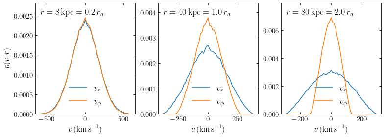
We see that at \(r/r_a \ll 1\), the distribution of \(v_r\) and \(v_\phi\) is approximately the same, but as \(r/r_a\approx 1\) and \(r/r_a > 1\), the distribution of velocities becomes increasingly radial, with a wide distribution of \(v_r\) accompanied by a narrow distribution of \(v_\phi\) around \(v_\phi=0\).
The Osipkov-Merritt distribution functions \(f(Q)\) can be further generalized to a form \(f(\mathcal{E},L) = f(Q)\,L^{-2\beta}\) which have \(\beta(r=0) = \beta\) and can therefore be used to model systems with tangential bias in their centers that transition to a radial bias in their outskirts. Such models can be constructed using a combination of the inversion techniques from this and the previous section (Cuddeford 1991).