14. Orbits in triaxial mass distributions and surfaces of section

\label{chap-triaxialorbits}

Orbits in axisymmetric potentials are relatively simple (Chapter 10): because of the conservation of the \(z\) component of the angular momentum, \(L_z\), all orbits with non-zero \(L_z\) loop around the \(z\) axis in either clockwise or counterclockwise direction. Orbits with \(L_z = 0\) are polar orbits, which reach their maximum height \(z_\mathrm{max}\) at \(R=0\). In Chapter 10.2, we argued that orbits in galactic axisymmetric potentials typically satisfy a third integral \(I_3\) of the motion in addition to \(E\) and \(L_z\); this third integral means that the orbits are all highly regular.

Orbits in triaxial mass distributions are typically more complicated than those in axisymmetric distributions. For a general triaxial mass distribution, no component of the angular momentum is conserved and orbits with non-zero initial angular momentum therefore do not have to maintain a well-defined sense of rotation. For a static triaxial potential, only the energy is a classical integral of the motion that restricts an orbit’s trajectory to a five-dimensional volume of phase-space. In general, we expect orbits to fill this entire five-dimensional subspace, unless there are additional, non-classical integrals that restrict the motion further—like for the third integral for axisymmetric potentials.

In this chapter, we discuss the types of orbits that exist in static triaxial gravitational potentials. Once we lift the restriction of axisymmetry, the types of orbits that can exist and their structure rapidly becomes more complex. To better study orbits, we therefore first introduce a more sophisticated tool than the simple orbit projections that we have relied on so far: surfaces of section. Along the way, we will also return to a question that we posed in Chapter 10.2 : Do all orbits in an axisymmetric potential have a third integral of motion?

14.1. Surfaces of section

\label{sec-sos}

Orbits in three-dimensional potentials are trajectories in six-dimensional phase-space. We have so far only discussed orbits in spherical potentials and axisymmetric potentials, where the symmetry of the potential allows one to get a reasonable projection of the orbit when viewed in just two of the six phase-space coordinates. However, when we consider orbits in triaxial potentials or when we want to more closely inspect the orbital structure of spherical and axisymmetric potentials, a better visualization of the orbits is in order. Here we discuss a standard method for visualizing the orbital structure of gravitational potentials and use it first to reconsider the orbits in disk potentials that we first discussed in Chapter 10. As in that chapter, we consider axisymmetric potentials that are symmetric with respect to rotation around the \(z\) axis and mirror-symmetric around \(z=0\).

Orbits in static axisymmetric potentials have two integrals of the motion: the energy \(E\) and the \(z\) component \(L_z\) of the angular momentum. As discussed in Chapter 10.1 (see also Chapter 5.3), the motion in \((\phi,v_\phi)\) is directly determined from \((L_z,R[t])\) through the conservation of \(L_z\) and we can thus fully investigate the orbital structure by considering only the four-dimensional phase-space \((R,z,v_R,v_z)\) in the meridional plane. In this four-dimensional space, the energy integral confines the orbit to a three-dimensional volume. We can choose to visualize this volume in \((R,z,v_R)\), because the energy fixes \(v_z\) given \((R,z,v_R)\) (the energy only fixes \(v_z\) up to a sign and we thus pick one of the possible signs, say the positive one). We can easily visualize this three-dimensional volume, by taking a slice through it at \(z=0\); this is called a surface of section. It is well-defined for an axisymmetric potential, because every orbit passes through \(z=0\). A two-dimensional slice through a three-dimensional volume generically fills a two-dimensional area and this is what we expect to see.

As an example, we consider the same orbit that we displayed in Chapter 10.1 (the first orbit we discussed with \(E=-1.25\)). We take the simple function to compute the surface of section defined in Bovy (2015). The surface of section of this orbit is

from galpy import potential
from galpy.orbit import Orbit
def orbit_RvRELz(R,vR,E,Lz,pot=None):
    """Returns Orbit at (R,vR,phi=0,z=0) with given (E,Lz)"""
    return Orbit([R,vR,Lz/R,0.,
                  numpy.sqrt(2.*(E-potential.evaluatePotentials(pot,R,0.)
                                 -(Lz/R)**2./2.-vR**2./2)),0.],ro=8.,vo=220.)
def surface_section(Rs,zs,vRs):
    # Find points where the orbit crosses z from - to +
    shiftzs= numpy.roll(zs,-1)
    indx= (zs[:-1] < 0.)*(shiftzs[:-1] > 0.)
    return (Rs[:-1][indx],vRs[:-1][indx])
R, E, Lz= 0.8, -1.25, 0.6
vR= 0.
o= orbit_RvRELz(R,vR,E,Lz,pot=potential.MWPotential2014)
ts= numpy.linspace(0.,100.,10001)
o.integrate(ts,potential.MWPotential2014)
sect1Rs,sect1vRs=surface_section(o.R(ts),o.z(ts),o.vR(ts))
plot(sect1Rs,sect1vRs,'o',mec='none')
xlabel(r'$R\,(\mathrm{kpc})$')
ylabel(r'$v_R\,(\mathrm{km\,s}^{-1})$');

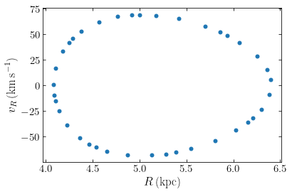
We see that the orbit does not appear to fill a two-dimensional area, but is instead confined to a one-dimensional curve. Even if we integrate the orbit for many more dynamical times this observation does not change:

ts= numpy.linspace(0.,3000.,300001)
o.integrate(ts,potential.MWPotential2014)
sect1Rs,sect1vRs=surface_section(o.R(ts),o.z(ts),o.vR(ts))
plot(sect1Rs,sect1vRs,'o',mec='none')
xlabel(r'$R\,(\mathrm{kpc})$')
ylabel(r'$v_R\,(\mathrm{km\,s}^{-1})$');

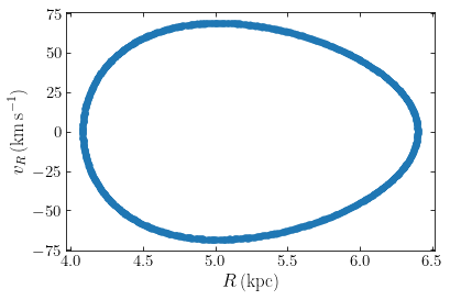
Thus, the locus of the orbit in the surface of section is one-dimensional, which means that the locus of the orbit in the three-dimensional \((R,z,v_R)\) space is only two-dimensional, a shell. The motion must therefore be confined to this two-dimensional subspace by an integral of the motion in addition to the energy and the \(z\) component of the angular momentum. The surface of section offers more direct support for this than simply looking at the orbit in the \((R,z)\) plane as we did in Chapter 10.1. This third integral is non-classical, because it does not follow from a symmetry of the potential, like for the energy (from time invariance) and \(L_z\) (from axisymmetry).

To visualize all of the possible orbits with \(E\) and \(L_z\) of the orbit above, we generate surfaces of section for six orbits ranging from having all available initial kinetic energy in the \(v_R\) component to having this all in the \(v_z\) component. This generates the following sequence of curves:

ts= numpy.linspace(0.,3000.,300001)
def maxvR_RELz(R,E,Lz,pot=None):
    """Returns maximum v_R for orbit at (R,phi=0,z=0) with given (E,Lz)"""
    return numpy.sqrt(2.*(E-potential.evaluatePotentials(pot,R,0.))-(Lz/R)**2.)
R, E, Lz= 0.8, -1.25, 0.6
vRs= numpy.sqrt(numpy.linspace(0.,maxvR_RELz(R,E,Lz,pot=potential.MWPotential2014)**2.,7))
for vR in vRs:
    o= orbit_RvRELz(R,vR,E,Lz,pot=potential.MWPotential2014)
    o.integrate(ts,potential.MWPotential2014)
    sect1Rs,sect1vRs=surface_section(o.R(ts),o.z(ts),o.vR(ts))
    plot(sect1Rs,sect1vRs,'.',mec='none')
xlabel(r'$R\,(\mathrm{kpc})$')
ylabel(r'$v_R\,(\mathrm{km\,s}^{-1})$');

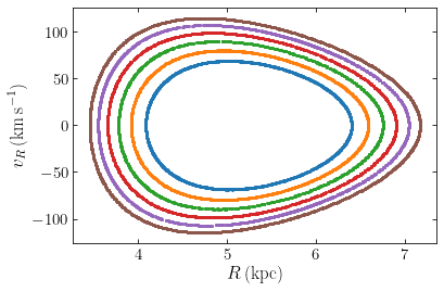
The innermost contour, which has all initial available kinetic energy in \(v_z\), is the same as that shown above. The other contours have more and more initial kinetic energy in \(v_R\). All of the orbits at this \((E,L_z)\) are confined between the innermost and outermost curves shown here and we see that all orbits form a closed, one-dimensional curve in the surface of section.

Another way to look at the orbital structure is to consider orbits at constant specific energy \(E\), but that vary \(L_z\) between a value close to zero and the maximum value for this \(E\) (which happens at the circular orbit with this \(E\)). To display only a single orbit at each \(L_z\) among the continuum of orbits at \((E,L_z)\), we always choose the orbit that has half of its initially-available kinetic energy in the \(v_z\) component and half in \(v_R\) (the middle orbit in the previous figure).

from scipy import optimize
def maxLz_E(E,pot=None):
    """Returns (R,Lz) for the circular orbit with energy E"""
    rE= optimize.brentq(lambda R: potential.evaluatePotentials(pot,R,0.)
                        +potential.vcirc(pot,R)**2./2.-E,0.01,2.)
    return (rE,rE*potential.vcirc(pot,rE))
ts= numpy.linspace(0.,3000.,300001)
E= -1.25
Rc, maxLz= maxLz_E(E,pot=potential.MWPotential2014)
Lzs= numpy.linspace(0.05,maxLz-0.000001,7) #v. close to circular
for Lz in Lzs:
    o= orbit_RvRELz(Rc,
                    maxvR_RELz(Rc,E,Lz,pot=potential.MWPotential2014)\
                        /numpy.sqrt(2.),
                    E,Lz,pot=potential.MWPotential2014)
    o.integrate(ts,potential.MWPotential2014)
    sect1Rs,sect1vRs=surface_section(o.R(ts),o.z(ts),o.vR(ts))
    if Lz == Lzs[-1]:
        plot(sect1Rs,sect1vRs,'o',mec='none')
    else:
        plot(sect1Rs,sect1vRs,'.',mec='none')
xlabel(r'$R\,(\mathrm{kpc})$')
ylabel(r'$v_R\,(\mathrm{km\,s}^{-1})$');

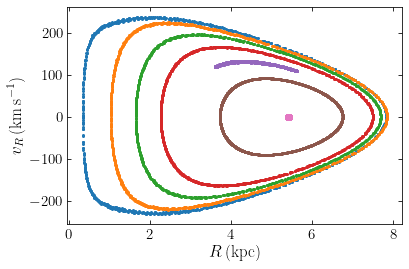
We can learn a lot about the orbits in the axisymmetric Milky-Way potential MWPotential2014 used to create this diagram. The innermost orbit has the maximum \(L_z\) for this energy and this is a circular orbit. The surface of section therefore reduces to a point. The other orbits generate one-dimensional curves that typically loop around this circular orbit; we say that the circular orbit is the parent orbit of this family of orbits. The loops get bigger and bigger as \(L_z\) decreases, with the lowest \(L_z\) orbit (the outermost curve) getting quite close to the center of the potential. The bulge component in MWPotential2014 ranges out to \(r = 1.9\,\mathrm{kpc}\); the lowest \(L_z\) orbit enters the bulge region where the potential is quite different from that in the disk and halo region (where the other orbits in this diagram orbit) which leads to the kink toward smaller \(|v_R|\) at \(R \lesssim 1.9\,\mathrm{kpc}\).

All but one of the orbits in the above diagram loop around the parent orbit in a regular fashion. The exception is the third orbit starting from the center (the purple curve). This orbit only covers part of a loop. Such partial loops in a surface of section are indicative of a resonant orbit: an orbit whose fundamental orbital frequencies—generalizations of the epicycle frequencies that we discussed in Chapter 10.3.1 (see Chapter 4.4.3)—are commensurate such that these orbits cannot cover their entire allowed phase-space volume (even after taking into account the third integral). Let’s take a closer look at this orbit:

figsize(9,5)
ts= numpy.linspace(0.,100.,10001)
Lz= Lzs[-3]
o= orbit_RvRELz(Rc,maxvR_RELz(Rc,E,Lz,pot=potential.MWPotential2014)\
                        /numpy.sqrt(2.),
                E,Lz,pot=potential.MWPotential2014)
o.integrate(ts,potential.MWPotential2014)
subplot(1,2,1)
o.plot(gcf=True)
subplot(1,2,2)
o.plot(d1='vR',d2='vz',gcf=True)
tight_layout();

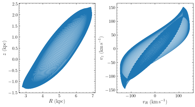
We see that this orbit is indeed resonant. Unlike the orbits that we displayed in Chapter 10.1, there is a clear correlation between the radial and vertical components of the orbit, due to the commensurability of the radial and vertical frequencies. Another way to display this is in the projection of the orbit in the \((v_R,v_z)\) plane, shown on the right.

Such resonant orbits are a common feature of galactic potentials and they occur more frequently and with much more variety in triaxial potentials. Resonances can make phase-space complicated in their surroundings, but this particular resonant orbit does not “affect” too much of phase space in this way. To demonstrate this, we zoom in around this orbit in the surface of section above:

figsize(5,5)
ts= numpy.linspace(0.,3000.,300001)
E= -1.25
Rc, maxLz= maxLz_E(E,pot=potential.MWPotential2014)
# Previous Lzs, we want to zoom in around the third from the end
Lzs= numpy.linspace(0.05,maxLz-0.000001,7) #v. close to circular
Lzs= numpy.linspace(Lzs[-3]-0.03,Lzs[-3]+0.03,5)
for Lz in Lzs:
    o= orbit_RvRELz(Rc,
                    maxvR_RELz(Rc,E,Lz,pot=potential.MWPotential2014)\
                        /numpy.sqrt(2.),
                    E,Lz,pot=potential.MWPotential2014)
    o.integrate(ts,potential.MWPotential2014)
    sect1Rs,sect1vRs=surface_section(o.R(ts),o.z(ts),o.vR(ts))
    plot(sect1Rs,sect1vRs,'.',mec='none')
xlabel(r'$R\,(\mathrm{kpc})$')
ylabel(r'$v_R\,(\mathrm{km\,s}^{-1})$');

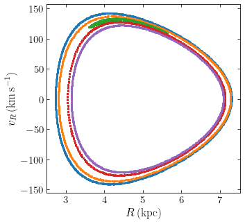
This diagram displays 2 orbits with slightly higher \(L_z\) and two orbits with slightly lower \(L_z\). As is clear, these are regular, non-resonant orbits that loop around the parent circular orbit (not shown).

Thus, orbital surfaces of section are highly useful diagnostics of the orbital structure of galactic potentials. For the axisymmetric potentials, they clearly demonstrate that most orbits must have a non-classical third integral of motion and they provide a simple manner to find resonant orbits.

14.2. Orbits in two-dimensional, non-axisymmetric systems

\label{sec-triaxialorbits-2dnonaxi}

To commence our exploration of orbits in triaxial systems, we first consider orbits in a two-dimensional, non-axisymmetric system (see Sec. 3.3.1 of Binney & Tremaine 2008) and introduce a new type of orbits that is important in triaxial systems. We consider a non-axisymmetric version of the logarithmic potential that we first discussed in Chapter 3.4.5 by deforming the potential in the \(y\) direction as

\begin{equation}\label{eq-nonaxi-logpot-planar} \Phi(x,y) = \frac{v_c^2}{2}\,\ln\left[x^2+\frac{y^2}{b^2}+R_c^2\right]\,, \end{equation}

where in addition to the non-axisymmetry (for \(b\neq 1\)) we have also introduced a core radius \(R_c\) (see also Chapter 9.1.6). At \(x,y \gg R_c\) and \(b \approx 1\), this potential approaches the logarithmic potential from Chapter 3.4.5 in the \(z=0\) plane. As an example, we consider the potential in Equation \(\eqref{eq-nonaxi-logpot-planar}\) with \(v_c = 1\), \(b=0.9\), and \(R_c = 0.2\). We start by looking at an orbit starting at \((x,y) = (0.1,0)\) with \(v_x = 0\) and \(v_y\) equal to the circular velocity at the initial \(x\) if the potential were axisymmetric:

from galpy.potential import LogarithmicHaloPotential
from galpy.orbit import Orbit
ts= numpy.linspace(0.,30,601)
lp= LogarithmicHaloPotential(normalize=True,b=0.9,core=0.2)
o= Orbit([0.1,0.,lp.vcirc(0.1,phi=0.),0.])
o.integrate(ts,lp)
o.animate(staticPlot=True); # remove the ; to display the animation

Play

Pause

Speed x 2

Speed / 2

Replay

If you play the animation, you see that this orbit does not loop around the center like orbits in an axisymmetric potential, but instead the orbit goes back and forth between clockwise and counterclockwise rotation. It is also clear that this orbit can approach the center arbitrarily closely, again in marked contrast to orbits with non-zero angular momentum in an axisymmetric potential, which are inhibited from doing so by the angular-momentum barrier.

To understand this type of orbit, we consider the potential at small distances from the center. At \(x,y \ll R_c\), the potential becomes

\begin{equation}\label{eq-triaxialorbits-2dnonaxi-approxlogpot} \Phi(x,y) \approx \frac{v_c^2}{2\,R_c^2}\,\left[x^2+\frac{y^2}{b^2}\right]\,. \end{equation}

This potential can be separated in \(x\) and \(y\) as \(\Phi(x,y) = \Phi_x(x)+\Phi_y(y) = \frac{v_c^2}{2\,R_c^2}\,x^2 + \frac{v_c^2}{2\,R_c^2\,b^2} y^2\); \(\Phi_x(x)\) and \(\Phi_y(y)\) are both the potential of a harmonic oscillator, albeit with different frequencies \(\omega_x = v_c/R_c\) and \(\omega_y = v_c/[R_c\,b]\) in the \(x\) and \(y\) directions, respectively. The motion in \(x\) and that in \(y\) therefore separates into two independent motions in each of \((x,v_x)\) and \((y,v_y)\). Unless \(\omega_x/\omega_y = b\) is a rational number, orbits do not close in the \((x,y)\) plane. Because each of the \(x\) and \(y\) oscillations covers a region between \((-x_\mathrm{max},x_\mathrm{max})\) and \((-y_\mathrm{max},y_\mathrm{max})\), respectively, the orbit in \((x,y)\) covers the entire box between the corners formed by the four combinations of the signs in \((\pm x_\mathrm{max},\pm y_\mathrm{max})\). As an example of this behavior, we look at the same potential as above, but now start an orbit well within the \(x,y \ll R_c\) regime, at \((x,y) = (0.01,0)\), again with \(v_x =0\) and \(v_y\) equal to the circular velocity at \(x\) in the axisymmetric (\(b=1\)) version of this potential. The orbit in \((x,y)\) looks as follows:

from galpy.potential import LogarithmicHaloPotential
from galpy.orbit import Orbit
ts= numpy.linspace(0.,30,601)
lp= LogarithmicHaloPotential(normalize=True,b=0.9,core=0.2)
o= Orbit([0.01,0.,lp.vcirc(0.01,phi=0.),0.])
o.integrate(ts,lp)
figsize(5,5)
o.plot()
gca().set_aspect('equal');

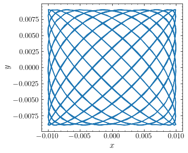
Thus, the orbit indeed fills a rectangular box in the \((x,y)\) plane. Note that in this example, \(b\) is a rational number and the orbit of objects at \(x,y \ll R_c\) therefore almost closes. But the anharmonicity resulting from deviations of the true potential from the approximation in Equation \eqref{eq-triaxialorbits-2dnonaxi-approxlogpot} causes the orbits to not close exactly and slowly fill the box. If you change \(b\) even slightly away from \(0.9\) in the example above, you will see that it fills the box much more quickly (for example, try \(b = \pi/3.5 \approx 0.8976\)).

As we approach \(x,y \approx R_c\), the potential no longer separates into the two harmonic-oscillator components like above, but orbits qualitatively keep following the same behavior: they oscillate between clockwise and counterclockwise rotation—and thus have \(\langle L_z \rangle \approx 0\)—and can approach the center arbitrarily closely. They no longer fill a rectangular box, but still fill a box-like region near the center that fans out at larger \((x,y)\); because of this, all such orbits are known as box orbits. The orbit that we animated above is an example of this:

from galpy.potential import LogarithmicHaloPotential
from galpy.orbit import Orbit
ts= numpy.linspace(0.,30,1001)
lp= LogarithmicHaloPotential(normalize=True,b=0.9,core=0.2)
o= Orbit([0.1,0.,lp.vcirc(0.1,phi=0.),0.])
o.integrate(ts,lp)
figsize(9,4.5)
subplot(1,2,1)
o.plot(gcf=True)
gca().set_aspect('equal')
subplot(1,2,2)
o.plot(d1='t',d2='Lz',ylabel=r'$L_z$',gcf=True)
ts= numpy.linspace(0.,300,10001)
o.integrate(ts,lp)
axhline(numpy.mean(o.Lz(ts)),color='k',ls='--')
galpy_plot.text(26.,-0.01,r'$\langle L_z \rangle$',size=18.)
tight_layout();

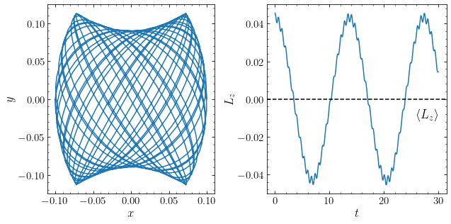
The run of the angular momentum as a function of time demonstrates that this orbit has no definite sense of rotation; the average value \(\langle L_z \rangle\) of its angular momentum is zero (the dashed line in the figure shows the long-term average of \(L_z\)).

When we consider orbits at \(x,y \gg R_c\), we find that the orbits do have a well-defined sense of rotation and loop around the center similar to an orbit in an axisymmetric potential. For example, look at the following orbit which has initial \((x,y) = (0.25,0)\) and velocities initialized with a similar procedure as above:

from galpy.potential import LogarithmicHaloPotential
from galpy.orbit import Orbit
ts= numpy.linspace(0.,30,1001)
lp= LogarithmicHaloPotential(normalize=True,b=0.9,core=0.2)
o= Orbit([0.25,0.,lp.vcirc(0.25,phi=0.),0.])
o.integrate(ts,lp)
o.animate(staticPlot=True); # remove the ; to display the animation

Play

Pause

Speed x 2

Speed / 2

Replay

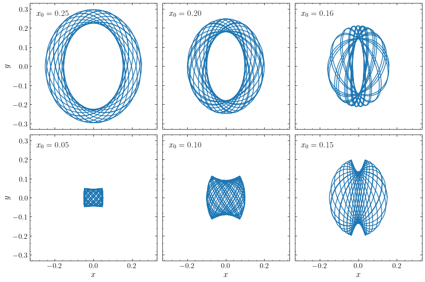
This orbit looks like a regular orbit in an axisymmetric potential and is known as a loop orbit. If we consider a sequence of orbits initialized in the manner above (that is, starting from \((x,y) = (x_0,0)\), with \(v_x = 0\) and \(v_y\) the circular velocity at \(x_0\) in the potential with \(b=1\)), then we see that the orbits go from loop orbits at \(x_0 \gg R_c\) to box orbits at \(x_0 \ll R_c\), with the switch for this family happening around \(x_0 \approx 0.16\). At that point, the loop orbit becomes highly eccentric and turns into a box orbit when \(x_0\) is slightly decreased (third and fourth panel going clockwise):

from galpy.potential import LogarithmicHaloPotential
from galpy.orbit import Orbit
ts= numpy.linspace(0.,30,1001)
figsize(12,8)
lp= LogarithmicHaloPotential(normalize=True,b=0.9,core=0.2)
xinit= [0.25,0.2,0.16,0.15,0.1,0.05]
for ii,xi in enumerate(xinit):
    o= Orbit([xi,0.,lp.vcirc(xi,phi=0.),0.])
    o.integrate(ts,lp)
    if ii > 2: ii= 8-ii # flip bottom row
    subplot(2,3,ii+1)
    if ii %3 == 0: tylabel= r'$y$'
    else: tylabel= None
    if ii < 3: txlabel= None
    else: txlabel= r'$x$'
    o.plot(gcf=True,
           xlabel=txlabel,ylabel=tylabel,
           xrange=[-.33,0.33],yrange=[-0.33,0.33]);
    if ii%3 > 0:
        gca().yaxis.set_major_formatter(NullFormatter())
    if ii< 3:
        gca().xaxis.set_major_formatter(NullFormatter())
    galpy_plot.text(r'$x_0 = {0:.2f}$'.format(xi),
                    top_left=True,size=17.)
tight_layout()

We can also study orbits in this sequence using a surface of section. For this two-dimensional potential, we can define a surface of section in an analogous way to how we defined it for the meridional plane in an axisymmetric potential above. We can reduce the four-dimensional phase-space from \((x,y,v_x,v_y)\) to \((x,y,v_x)\) by using the conservation of energy (and breaking the sign degeneracy by only keep the positive \(v_y\) solution); then we look at the surface \(y=0\). For the sequence defined above, that gives the following sequence of curves in the surface of section:

figsize(9,6)
from matplotlib import cm
def surface_section(xs,ys,vxs):
    # Find points where the orbit crosses y from - to +
    shiftys= numpy.roll(ys,-1)
    indx= (ys[:-1] < 0.)*(shiftys[:-1] > 0.)
    return (xs[:-1][indx],vxs[:-1][indx])
ts= numpy.linspace(0.,1000.,1000001)
lp= LogarithmicHaloPotential(normalize=True,b=0.9,core=0.2)
xinit= numpy.linspace(-0.25,0.25,21)
for xi in xinit:
    o= Orbit([xi,0.,lp.vcirc(xi,phi=0.),0.])
    o.integrate(ts,lp)
    sectxs,sectvxs=surface_section(o.x(ts),o.y(ts),o.vx(ts))
    plot(sectxs,sectvxs,'.',mec='none',
         mfc=cm.viridis(numpy.fabs(xi/numpy.amax(xinit))))
xlabel(r'$x$')
ylabel(r'$v_x$');

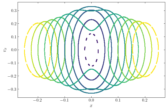
The curves go through the sequence \(x_0 = -0.25\) to \(x_0=0.25\) in steps with \(\Delta x_0 = 0.025\) and the curves are color-coded by \(|x_0|\). We see that each orbit gives rise to a one-dimensional curve, indicating that each orbit satisfies an integral of the motion beyond the classical energy (a second, non-classical integral in this case). The curves that loop around \(x \neq 0\) are the loop orbits, looping either counterclockwise or clockwise (for positive and negative \(x_0\), respectively). The curves that loop around the center are the box orbits. The curves for the loop and box orbits are all quite simple, except for the box orbits that are the closest to the loop orbits, which display somewhat more interesting behavior.

A better way to study the orbital structure of this non-axisymmetric potential is to look at surfaces of section of orbits with a fixed specific energy \(E\). The following figure displays the surface of section for \(E=-0.87\), the energy of the outermost loop orbit above:

from scipy import optimize
from galpy.potential import evaluatePotentials
def orbit_xvxE(x,vx,E,pot=None):
    """Returns Orbit at (x,vx,y=0) with given E"""
    return Orbit([x,vx,numpy.sqrt(2.*(E-evaluatePotentials(pot,x,0.,phi=0.)
                                  -vx**2./2)),0.])
def zvc(x,E,pot=None):
    """Returns the maximum v_x at this x and this
       energy: the zero-velocity curve"""
    return numpy.sqrt(2.*(E-evaluatePotentials(pot,x,0.,phi=0.)))
lp= LogarithmicHaloPotential(normalize=True,b=0.9,core=0.2)
E= -0.87
x= 0.204
maxvx= zvc(x,E,pot=lp)
vxs= numpy.linspace(0.,maxvx-1e-10,11)
ts= numpy.linspace(0.,1000.,1000001)
for vx in vxs:
    for sgn in [-1,1]:
        o= orbit_xvxE(sgn*x,vx,E,pot=lp)
        o.integrate(ts,lp)
        sectxs,sectvxs=surface_section(o.x(ts),o.y(ts),o.vx(ts))
        if vx == vxs[0]: marker= 'o'
        else: marker= '.'
        plot(sectxs,sectvxs,marker,mec='none',zorder=2,
             mfc=cm.viridis(numpy.fabs(vx/numpy.amax(vxs))))
# Also plot the zero-velocity curve, first find min x at which it exists
minx= optimize.brentq(lambda x: E-evaluatePotentials(lp,x,0.,phi=0.),
                     0.2,0.4)-1e-10
xs= numpy.linspace(-minx,minx,201)
plot(xs,zvc(xs,E,pot=lp),color=cm.viridis(1.),zorder=0)
plot(xs,-zvc(xs,E,pot=lp),color=cm.viridis(1.),zorder=1)
galpy_plot.text(r'$b=0.9$',top_left=True,size=18.)
xlabel(r'$x$')
ylabel(r'$v_x$');

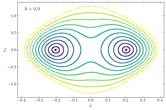
This surface of section again shows the two types of orbits. The loop orbits with positive and negative average angular momentum are the loops around \(x\approx \pm 0.204\); the orbit with \((x,v_x) = (0.204,0)\) is the closed loop orbit, which is the parent of this family of loop orbits. The orbits that loop around the center are again box orbits; at constant energy, they circulate around the center in greater loops than the loop orbits. The outermost curve has the maximum amount of energy in the \(x\) component: it has \(v_y \equiv 0\) at all times and thus oscillates back and forth along the \(x\) axis. This orbit is the closed long-axis orbit; it is an extreme version of the box orbits that we have seen in this section and is the parent of the family of box orbits at this energy (analogous to how the closed loop orbit is the parent of the loop orbits). The path of the closed long-axis orbit in the surface of section is a type of zero-velocity curve, because we can obtain the path from the equation \(v_y=0\); we compute and show this as the solid line above.

Because both the closed loop and the closed long-axis orbit give rise to families of orbits in their vicinity, they are both stable orbits in the sense that a small perturbation to these parent orbits gives a perturbed orbit in the same family as the parent. This is different from the situation for an axisymmetric potential (say, the logarithmic potential that we are considering here with \(b=1\)): the closed long-axis orbit exists in the axisymmetric potential (and has \(L_z=0\)), but any perturbation to it results in a loop orbit, because all orbits with \(L_z \neq 0\) in an axisymmetric potential are loop orbits.

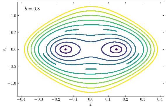
If we increase the level of non-axisymmetry, the importance of box orbits at a given energy increases. For example, the following is the surface of section at the same energy \(E=-0.87\) as above, but for the logarithmic potential that thas \(b=0.8\).

from scipy import optimize
def orbit_xvxE(x,vx,E,pot=None):
    """Returns Orbit at (x,vx,y=0) with given E"""
    return Orbit([x,vx,numpy.sqrt(2.*(E-evaluatePotentials(pot,x,0.,phi=0.)
                                  -vx**2./2)),0.])
def zvc(x,E,pot=None):
    """Returns the maximum v_x at this x and this
       energy: the zero-velocity curve"""
    return numpy.sqrt(2.*(E-evaluatePotentials(pot,x,0.,phi=0.)))
lp= LogarithmicHaloPotential(normalize=True,b=0.8,core=0.2)
E= -0.87
x= 0.147
maxvx= zvc(x,E,pot=lp)
vxs= numpy.linspace(0.,maxvx-1e-10,11)
ts= numpy.linspace(0.,1000.,1000001)
for vx in vxs:
    for sgn in [-1,1]:
        o= orbit_xvxE(sgn*x,vx,E,pot=lp)
        o.integrate(ts,lp)
        sectxs,sectvxs=surface_section(o.x(ts),o.y(ts),o.vx(ts))
        if vx == vxs[0]: marker= 'o'
        else: marker= '.'
        plot(sectxs,sectvxs,marker,mec='none',zorder=2,
             mfc=cm.viridis(numpy.fabs(vx/numpy.amax(vxs))))
# Also plot the zero-velocity curve, first find min x at which it exists
minx= optimize.brentq(lambda x: E-evaluatePotentials(lp,x,0.,phi=0.),
                     0.2,0.4)-1e-10
xs= numpy.linspace(-minx,minx,201)
plot(xs,zvc(xs,E,pot=lp),color=cm.viridis(1.),zorder=0)
plot(xs,-zvc(xs,E,pot=lp),color=cm.viridis(1.),zorder=1)
galpy_plot.text(r'$b=0.8$',top_left=True,size=18.)
xlabel(r'$x$')
ylabel(r'$v_x$');

Once we go to \(b=0.7\), there are almost no loop orbits left at this energy:

from scipy import optimize
def orbit_xvxE(x,vx,E,pot=None):
    """Returns Orbit at (x,vx,y=0) with given E"""
    return Orbit([x,vx,numpy.sqrt(2.*(E-evaluatePotentials(pot,x,0.,phi=0.)
                                  -vx**2./2)),0.])
def zvc(x,E,pot=None):
    """Returns the maximum v_x at this x and this
       energy: the zero-velocity curve"""
    return numpy.sqrt(2.*(E-evaluatePotentials(pot,x,0.,phi=0.)))
lp= LogarithmicHaloPotential(normalize=True,b=0.7,core=0.2)
E= -0.87
x= 0.0555
maxvx= zvc(x,E,pot=lp)
vxs= numpy.linspace(0.,maxvx-1e-10,11)
ts= numpy.linspace(0.,1000.,1000001)
for vx in vxs:
    for sgn in [-1,1]:
        o= orbit_xvxE(sgn*x,vx,E,pot=lp)
        o.integrate(ts,lp)
        sectxs,sectvxs=surface_section(o.x(ts),o.y(ts),o.vx(ts))
        if vx == vxs[0]: marker= 'o'
        else: marker= '.'
        plot(sectxs,sectvxs,marker,mec='none',zorder=2,
             mfc=cm.viridis(numpy.fabs(vx/numpy.amax(vxs))))
# Also plot the zero-velocity curve, first find min x at which it exists
minx= optimize.brentq(lambda x: E-evaluatePotentials(lp,x,0.,phi=0.),
                     0.2,0.4)-1e-10
xs= numpy.linspace(-minx,minx,201)
plot(xs,zvc(xs,E,pot=lp),color=cm.viridis(1.),zorder=0)
plot(xs,-zvc(xs,E,pot=lp),color=cm.viridis(1.),zorder=1)
galpy_plot.text(r'$b=0.7$',top_left=True,size=18.)
xlabel(r'$x$')
ylabel(r'$v_x$');

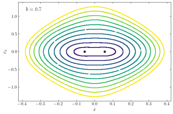
The same behavior occurs if we reduce the energy at constant \(b\): at lower energies, more of the phase-space is taken up by box orbits and the stable closed loop orbits move towards smaller \(|x|\), just like what happens when we decrease \(b\) in the figures above. At the same time, these closed loop orbits become more and more elliptical. At a certain critical energy, the closed loop orbits have \(x=0\) and morph into a closed short-axis orbit. This is expected from the asymptotic small \((x,y)\) behavior that we discussed above: orbits with low energies always remain at \(x,y \ll R_c\) where the potential is approximately that of two independent harmonic oscillators in \(x\) and \(y\); these have closed orbits at \((y,v_y)=(0,0)\), the closed long-axis box orbit, and at \((x,v_x)=(0,0)\), the closed short-axis box orbit. Conversely, when the energy increases, the closed short-axis box orbit turns into two closed loop orbits, one with clockwise and one with counterclockwise rotation. We say that the short-axis box orbit bifurcates into the closed loop orbit.

Loop and box orbits are the main families of orbits in static, two-dimensional non-axisymmetric potentials, with loop orbits the generalization of the stable orbits in axisymmetric potentials and the closed loop orbit the generalization of circular orbits. Before continuing our discussion of orbits in three-dimensional non-axisymmetric potential, we take a detour to learn about another important class of orbits: chaotic orbits.

14.3. Chaos in axisymmetric systems

\label{sec-sos-chaos-henonheiles}

The orbit families that we have discussed so far are all regular orbits: they all satisfy three (or two for the planar, non-axisymmetric potentials above) integrals of the motion—including one non-classical one—and they trace simple, smooth one-dimensional curves in the surface of section. Before turning our attention to orbits in triaxial mass distributions, we investigate whether all orbits in three-dimensional, axisymmetric systems or in two-dimensional, non-axisymmetric systems are regular. We will see that they are not: some orbits in some gravitational potentials do not satisfy a non-classical integral of the motion, but rather fill much of the volume of phase-space that is permitted by the conservation of their classical integrals of motion. Such orbits are referred to as ergodic (because for a non-axisymmetric system, only the conservation of energy remains for such orbits and systems for which only the energy matters are ergodic systems; see Chapter 6.6.1) or as chaotic.

To investigate whether all axisymmetric systems satisfy a third integral of the motion, we follow the classical paper by Henon & Heiles (1964), which was the first to demonstrate that this is not the case. As we discussed in Chapter 10.1, motion in an axisymmetric potential can be effectively reduced to the motion in a two-dimensional system in \((R,z)\), the meridional plane, with an effective potential given by the original potential plus a term proportional to the \(z\) component of the angular momentum. Such a system is effectively equivalent to a two-dimensional, non-axisymmetric system if we identify \((R,z) \rightarrow (x,y)\) and continue the potential to negative \(R\) by mirroring the potential \(\Phi(-R,z) = \Phi(R,z)\). Thus, to investigate whether or not an axisymmetric potential has orbits that do not conserve a third integral, we can equivalently study whether or not the effective two-dimensional, non-axisymmetric potential has orbits that do not conserve a second integral.

From this line of argument, Henon & Heiles (1964) further argued that we can simply study orbits in a simple two-dimensional potential if all we are interested in is an existence proof of ergodic orbits. The potential they proposed is

\begin{equation}\label{eq-pot-henon-heiles} \Phi(x,y) = \frac{1}{2}\,\left(x^2+y^2+2x^2y-\frac{2}{3}y^3\right)\,, \end{equation}

or in polar coordinates

\begin{equation} \Phi(R,\phi) = \frac{1}{2}\,\left[R^2+\frac{2\,R^3}{3}\,\sin\left(3\phi\right)\right]\,. \end{equation}

One could think of this as the potential in the meridional plane of (a) an orbit with \(L_z = 0\) (such that the \(L_z^2/[2\,R^2]\) term is absent) and (b) for a potential that is not mirror symmetric around the \(z=0\) plane. This is unlike the axisymmetric potentials that we have so far discussed and this is not a realistic model for a galactic potential. However, this simple system exhibits many of the phenomena of chaotic orbits that are important for chaotic orbits in more realistic galactic potential, so it still provides a useful starting point.

We start by considering orbits in the potential in Equation \(\eqref{eq-pot-henon-heiles}\) with energy \(E=1/12\). Using the techniques of the previous sections, we determine the surface of section for these orbits, this time fixing the \(v_x\) velocity from the conservation of energy and using crossings of the \(x=0\) plane to produce the surface of section in \((y,v_y)\). The surface of section looks as follows:

from galpy.potential import HenonHeilesPotential
from galpy import potential
from galpy.orbit import Orbit
from scipy import optimize
def surface_section(xs,ys,vys):
    # Find points where the orbit crosses x from - to +
    shiftxs= numpy.roll(xs,-1)
    indx= (xs[:-1] < 0.)*(shiftxs[:-1] > 0.)
    return (ys[:-1][indx],vys[:-1][indx])
def orbit_yvyE(y,vy,E,pot=None):
    """Returns Orbit at (x=0,vx,y,vy) with given E,
       with the initial point on the SOS (-sqrt...)"""
    return Orbit([y,vy,-numpy.sqrt(2.*(E-potential.evaluateplanarPotentials(pot,y,phi=numpy.pi/2.)
                                   -vy**2./2)),numpy.pi/2.])
def zvc(y,E,pot=None):
    """Returns the maximum v_y at this y and this
       energy: the zero-velocity curve"""
    return numpy.sqrt(2.*(E-potential.evaluateplanarPotentials(pot,y,phi=numpy.pi/2.)))
figsize(9,6)
hp= HenonHeilesPotential(amp=1.)
E= 1./12.
# Location in y of closed orbits
ys= [-.30375,0.255,1e-9]
ts= numpy.linspace(0.,10000.,1000001)
for y in ys:
    maxvy= zvc(y,E,pot=hp)
    if y > 0.01:
        vys= [0.,0.2041/2.,0.2041,maxvy]
    elif y < -0.01:
        vys= [0.,0.2041/2.,0.2041,maxvy]
    else:
        # 0.2041 is location of closed orbit at y=0
        vys= [0.2041,-0.2041,0.1641,-0.1641]
    for vy in vys:
        o= orbit_yvyE(y,vy,E,pot=hp)
        # Integrating some of these orbits is numerically tricky
        # so we use a very precise Dormand-Prince method
        o.integrate(ts,hp,method='dop853_c')
        sectys,sectvys=surface_section(o.x(ts),o.y(ts),o.vy(ts))
        if (numpy.fabs(y) > 0.01 and vy == vys[0]) \
            or (numpy.fabs(y) < 0.01 and numpy.fabs(numpy.fabs(vy)-0.2041) < 0.01):
            marker= 'o'
        else: marker= '.'
        if y < -0.01: mfc= '#d62728'
        elif y > +0.01: mfc= '#ff7f0e'
        elif vy > 0: mfc= '#1f77b4'
        else: mfc= '#2ca02c'
        plot(sectys,sectvys,marker,mec='none',zorder=2,mfc=mfc)
# Add the crossed curve, need to integrate longer
ts= numpy.linspace(0.,100000.,10000001)
o= orbit_yvyE(-0.1215,0.,E,pot=hp)
o.integrate(ts,hp)
sectys,sectvys=surface_section(o.x(ts),o.y(ts),o.vy(ts))
plot(sectys,sectvys,marker,mec='none',zorder=2,mfc='#9467bd')
# Also plot the zero-velocity curve
miny= optimize.brentq(lambda y: E-potential.evaluateplanarPotentials(hp,y,phi=numpy.pi/2.),
                     -0.4,-0.3)+1e-10
maxy= optimize.brentq(lambda y: E-potential.evaluateplanarPotentials(hp,y,phi=numpy.pi/2.),
                     0.4,0.6)-1e-10
ys= numpy.linspace(miny,maxy,201)
plot(ys,zvc(ys,E,pot=hp),color='k',zorder=10,lw=0.5)
plot(ys,-zvc(ys,E,pot=hp),color='k',zorder=11,lw=0.5)
xlabel(r'$y$')
ylabel(r'$v_y$');

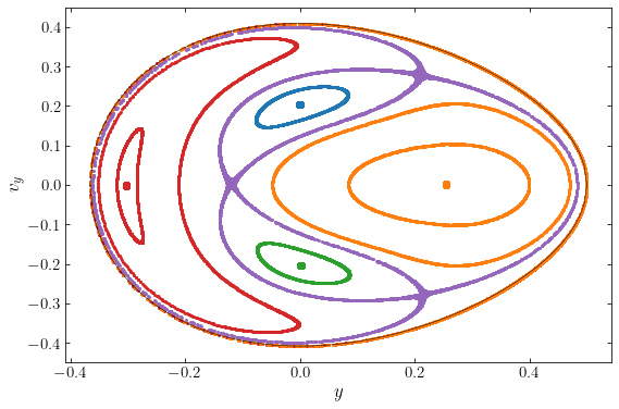
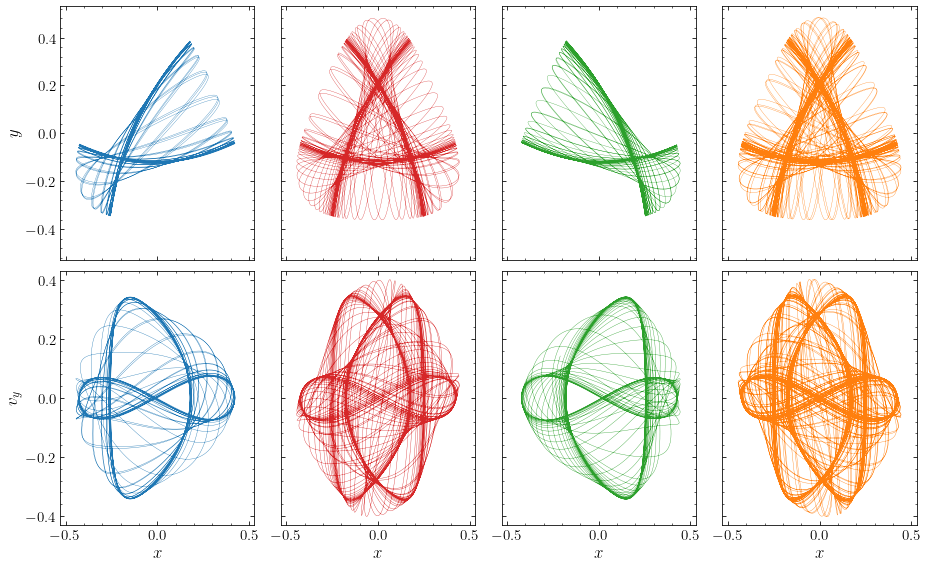
At \(E=1/12\) there are four stable, closed orbits that are the parents of orbits families; these are indicated by the large dots in the above figure. They span stable orbit families, indicated using the same color as the parents. These four closed orbits look as follows:

figsize(13,8)
hp= HenonHeilesPotential(amp=1.)
E= 1./12.
# Location in y of closed orbits
ys= [-.30375,0.255,1e-9,1e-9]
vys= [0.,0.,0.2041,-0.2041]
colors= ['#d62728','#ff7f0e','#1f77b4','#2ca02c']
ts= numpy.linspace(0.,30,1001)
for ii,(y,vy) in enumerate(zip(ys,vys)):
    o= orbit_yvyE(y,vy,E,pot=hp)
    o.integrate(ts,hp,method='dop853_c')
    subplot(2,4,ii+1)
    if ii == 0: tylabel= r'$y$'
    else: tylabel= None
    o.plot(gcf=True,
           xlabel=None,ylabel=tylabel,color=colors[ii],
           xrange=[-.53,0.53],yrange=[-0.53,0.53])
    if ii%4 > 0:
        gca().yaxis.set_major_formatter(NullFormatter())
    gca().xaxis.set_major_formatter(NullFormatter())
    if ii < 2:
        txtString= r'$(y_0,v_{{y,0}}) = ({0:.3f},{1:.1f})$'\
                            .format(y,vy)
    else:
        txtString= r'$(y_0,v_{{y,0}}) = ({0:.1f},{1:.4f})$'\
                            .format(y,vy)
    galpy_plot.text(txtString,top_left=True,size=17.)
    # Also plot (x,v_y)
    subplot(2,4,4+ii+1)
    if ii == 0: tylabel= r'$v_y$'
    else: tylabel= None
    o.plot(d1='x',d2='vy',gcf=True,
           xlabel=r'$x$',ylabel=tylabel,color=colors[ii],
           xrange=[-.53,0.53],yrange=[-0.43,0.43])
    if ii%4 > 0:
        gca().yaxis.set_major_formatter(NullFormatter())
tight_layout()

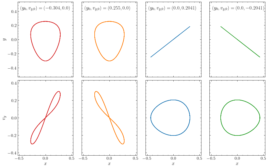
The closed orbits with \(v_y=0\) in the surface of section are the two left columns. These are loop orbits that loop around the origin in a fixed direction. Both of the closed loop orbits follow the same trajectory in \((x,y)\), but they go around this trajectory in opposite directions. This is directly analogous to the circular loop orbits in an two-dimensional axisymmetric potential.

The closed orbits with \(y=0\) in the surface of section are shown in the right two columns. They are needle-like, just like the long-axis box orbits above and they are therefore also box orbits.

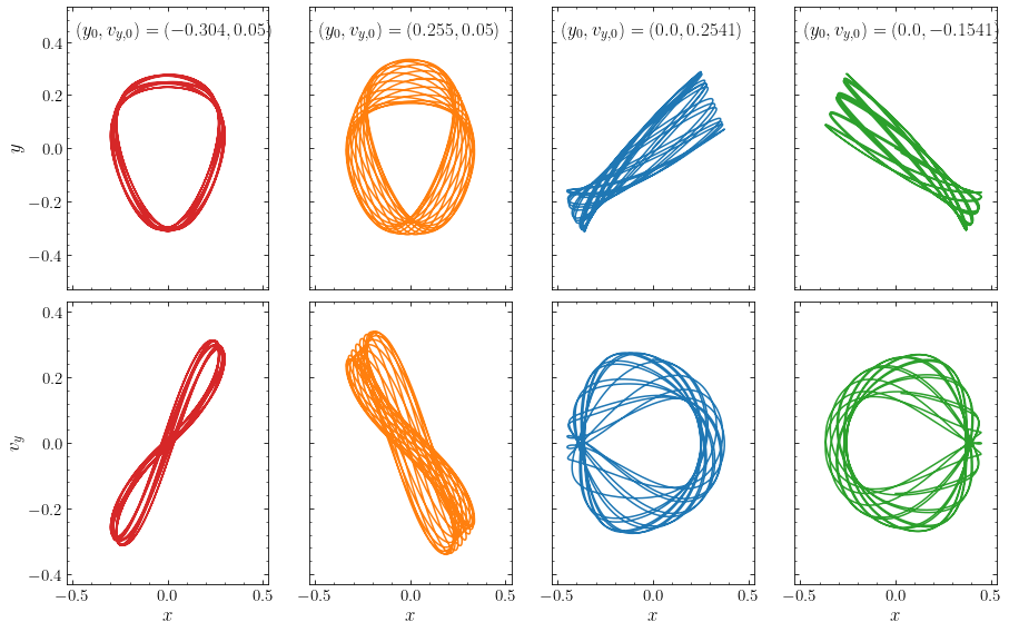
These four closed orbits are the parents of stable orbit families of loop orbits (for the left two columns above) and of box orbits (for the right two columns above). For example, if we perturb the initial velocity of these orbits by \(\Delta v_y = 0.05\) we obtain the following loop and box orbits that look similar to the loop and box orbits that we discussed above:

figsize(13,8)
hp= HenonHeilesPotential(amp=1.)
E= 1./12.
# Location in y of closed orbits
ys= [-.30375,0.255,1e-9,1e-9]
vys= [0.,0.,0.2041,-0.2041]
colors= ['#d62728','#ff7f0e','#1f77b4','#2ca02c']
# perturb
vys= [vy+0.05 for vy in vys]
ts= numpy.linspace(0.,100,3001)
for ii,(y,vy) in enumerate(zip(ys,vys)):
    o= orbit_yvyE(y,vy,E,pot=hp)
    o.integrate(ts,hp,method='dop853_c')
    subplot(2,4,ii+1)
    if ii == 0: tylabel= r'$y$'
    else: tylabel= None
    o.plot(gcf=True,color=colors[ii],
           xlabel=None,ylabel=tylabel,
           xrange=[-.53,0.53],yrange=[-0.53,0.53])
    if ii%4 > 0:
        gca().yaxis.set_major_formatter(NullFormatter())
    gca().xaxis.set_major_formatter(NullFormatter())
    if ii < 2:
        txtString= r'$(y_0,v_{{y,0}}) = ({0:.3f},{1:.2f})$'\
                            .format(y,vy)
    else:
        txtString= r'$(y_0,v_{{y,0}}) = ({0:.1f},{1:.4f})$'\
                            .format(y,vy)
    galpy_plot.text(txtString,top_left=True,size=17.)
    # Also plot (x,v_y)
    subplot(2,4,4+ii+1)
    if ii == 0: tylabel= r'$v_y$'
    else: tylabel= None
    o.plot(d1='x',d2='vy',gcf=True,color=colors[ii],
           xlabel=r'$x$',ylabel=tylabel,
           xrange=[-.53,0.53],yrange=[-0.43,0.43])
    if ii%4 > 0:
        gca().yaxis.set_major_formatter(NullFormatter())
tight_layout()

The purple curve in the surface of section above straddles the edge of all four stable orbit families. It goes between periods of time where it displays behavior similar to the box orbits above and episodes where it behaves more like the loop orbits above. For example, the following figure shows four episodes of duration \(\Delta t \approx \mathrm{few\ hundred}\) during a long orbit integration (with total \(\Delta t \approx 18,000\)):

tint= [300.,500.,300.,800.]
tinbetween= [3250.,9000.,3000.]
colors= ['#1f77b4','#d62728','#2ca02c','#ff7f0e']
o= orbit_yvyE(-0.1215,0.,E,pot=hp)
figsize(13,8)
for ii in range(4):
    ts= numpy.linspace(0.,tint[ii],200001)
    o.integrate(ts,hp,method='dop853_c')
    subplot(2,4,ii+1)
    if ii == 0: tylabel= r'$y$'
    else: tylabel= None
    o.plot(gcf=True,lw=0.3,
           xlabel=None,ylabel=tylabel,color=colors[ii],
           xrange=[-.53,0.53],yrange=[-0.53,0.53])
    if ii%4 > 0:
        gca().yaxis.set_major_formatter(NullFormatter())
    gca().xaxis.set_major_formatter(NullFormatter())
    # Also plot (x,v_y)
    subplot(2,4,4+ii+1)
    if ii == 0: tylabel= r'$v_y$'
    else: tylabel= None
    o.plot(d1='x',d2='vy',gcf=True,lw=0.35,
           xlabel=r'$x$',ylabel=tylabel,color=colors[ii],
           xrange=[-.53,0.53],yrange=[-0.43,0.43])
    if ii%4 > 0:
        gca().yaxis.set_major_formatter(NullFormatter())
    # Go to next loop
    if ii < 3:
        o= o(ts[-1])
        ts= numpy.linspace(0.,tinbetween[ii],200001)
        o.integrate(ts,hp,method='dop853_c')
        o= o(ts[-1])
tight_layout();

In the first and third episodes, the orbit behaves like a member of the box-orbit family, while in the second and fourth episode, the orbit looks more like a loop orbit. We can also loop at these four episodes in the surface of section:

figsize(9,6)
ts= numpy.linspace(0.,tint[0],20001)
# Start with top loop
o= orbit_yvyE(-0.1215,0.,E,pot=hp)
o.integrate(ts,hp,method='dop853_c')
sectys,sectvys=surface_section(o.x(ts),o.y(ts),o.vy(ts))
plot(sectys,sectvys,'o-',color=colors[0])
# Go to right loop
o= o(ts[-1])
ts= numpy.linspace(0.,tinbetween[0],20001)
o.integrate(ts,hp,method='dop853_c')
o= o(ts[-1])
ts= numpy.linspace(0.,tint[1],20001)
o.integrate(ts,hp,method='dop853_c')
sectys,sectvys=surface_section(o.x(ts),o.y(ts),o.vy(ts))
plot(sectys,sectvys,'o',color=colors[1],zorder=2)
# Go to bottom loop
o= o(ts[-1])
ts= numpy.linspace(0.,tinbetween[1],20001)
o.integrate(ts,hp,method='dop853_c')
o= o(ts[-1])
ts= numpy.linspace(0.,tint[2],20001)
o.integrate(ts,hp,method='dop853_c')
sectys,sectvys=surface_section(o.x(ts),o.y(ts),o.vy(ts))
plot(sectys,sectvys,'o-',color=colors[2],zorder=1)
# Go to left loop
o= o(ts[-1])
ts= numpy.linspace(0.,tinbetween[2],20001)
o.integrate(ts,hp,method='dop853_c')
o= o(ts[-1])
ts= numpy.linspace(0.,tint[3],20001)
o.integrate(ts,hp,method='dop853_c')
sectys,sectvys=surface_section(o.x(ts),o.y(ts),o.vy(ts))
plot(sectys,sectvys,'o',color=colors[3])
xlim(-0.4,0.55)
ylim(-0.45,0.45)
xlabel(r'$y$')
ylabel(r'$v_y$');

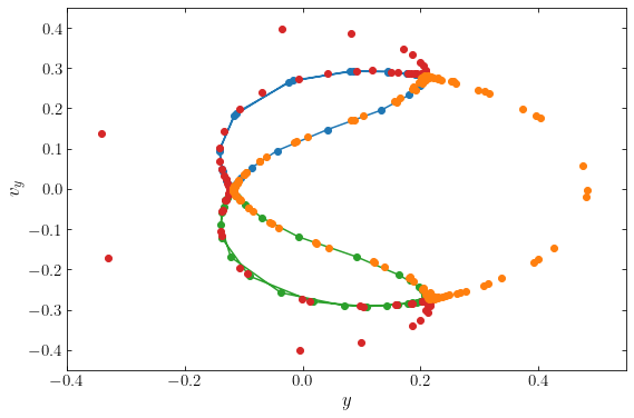
The orbit starts out as the blue curve (we have connected the dots to make this more clear), going around the closed box orbit with \(v_y > 0\) as if it were a member of that orbit’s family. The orbit then goes onto the locus given by the red dots (which we have not connected), like a member of the loop orbit family with \(y<0\). Then the orbit transitions to the green curve, like a member of the family of box orbits with \(v_y < 0\). Finally, the orbit goes onto the orange locus, as a member of the loop orbits with \(y > 0\). This orbit is unstable: any small perturbation will transform it into a bona-fide member of one of the four stable orbit families. This instability also manifests itself in the numerical orbit integration: even relative energy errors of \(10^{-11}\) cause small changes in the positions and velocities along the orbit that affect how the orbit transitions between the four different behaviors; if we slightly change the parameters of the numerical orbit integration, we get different behavior along the same orbit.

To even better understand this unstable orbit, it is instructive to look at an animation of it. The following animation shows orbit segments over a span of 15,000 time units

Play

Pause

Speed x 2

Speed / 2

Replay

You see that the orbit starts at with the behavior of the positive \(v_y\) box orbit and is stuck there for a long time. It then transitions to the counter-clockwise loop orbit, flips to the clockwise loop orbit, flips back to the counter-clockwise loop orbit, gets caught by the positive \(v_y\) box orbit, goes back to the counter-clockwise loop orbit, goes onto the negative \(v_y\) box orbit, and so on. It’s clear that the behavior is quite erratic, with no clear pattern of when and to what orbit famility the orbit will transition at any time.

All the orbits at \(E=1/12\) display one-dimensional curves in the surface of section and they are therefore all regular. However, this system is at the threshold of chaos. If we increase the energy to \(E=1/8\), the surface of section becomes the following:

from galpy.potential import HenonHeilesPotential
from galpy.orbit import Orbit
from scipy import optimize
def surface_section(xs,ys,vys):
    # Find points where the orbit crosses x from - to +
    shiftxs= numpy.roll(xs,-1)
    indx= (xs[:-1] < 0.)*(shiftxs[:-1] > 0.)
    return (ys[:-1][indx],vys[:-1][indx])
def orbit_yvyE(y,vy,E,pot=None):
    """Returns Orbit at (x=0,vx,y,vy) with given E,
       with the initial point on the SOS (-sqrt...)"""
    return Orbit([y,vy,-numpy.sqrt(2.*(E-potential.evaluateplanarPotentials(pot,y,phi=numpy.pi/2.)
                                   -vy**2./2)),numpy.pi/2.])
def zvc(y,E,pot=None):
    """Returns the maximum v_y at this y and this
       energy: the zero-velocity curve"""
    return numpy.sqrt(2.*(E-potential.evaluateplanarPotentials(pot,y,phi=numpy.pi/2.)))
figsize(9,6)
hp= HenonHeilesPotential(amp=1.)
E= 1./8.
# Location in y of closed orbits
ys= [-.37225,0.3025,1e-9,-0.08]
ts= numpy.linspace(0.,10000.,1000001)
for y in ys:
    maxvy= zvc(y,E,pot=hp)
    if y > 0.1:
        vys= [0.,0.25/8.,0.25/4.,0.113,0.25/2.,maxvy]
    elif y < -0.1:
        vys= [0.,0.25/2.,0.2]
    elif y < -0.01:
        vys= [-0.185,0.186]
    else:
        # 0.25 is location of closed orbit at y=0
        vys= [0.25,-0.25,0.22,-0.22,-0.19,0.19,0.38]
    for vy in vys:
        o= orbit_yvyE(y,vy,E,pot=hp)
        o.integrate(ts,hp)
        sectys,sectvys=surface_section(o.x(ts),o.y(ts),o.vy(ts))
        if (numpy.fabs(y) > 0.1 and vy == vys[0]) \
            or (numpy.fabs(y) < 0.1 and numpy.fabs(numpy.fabs(vy)-0.25) < 0.01):
            marker= 'o'
        else: marker= '.'
        if y < -0.1: mfc= '#d62728'
        elif y > +0.1: mfc= '#ff7f0e'
        elif vy > 0.37: mfc= '#d62728' # red island
        elif y < -0.01 and vy > 0: mfc= '#1f77b4'
        elif y < -0.01 and vy < 0: mfc= '#2ca02c'
        elif vy > 0: mfc= '#1f77b4'
        else: mfc= '#2ca02c'
        plot(sectys,sectvys,marker,mec='none',zorder=2,mfc=mfc)
# Add the chaotic regions, need to integrate longer
ts= numpy.linspace(0.,100000.,10000001)
oc= orbit_yvyE(-0.1,0.,E,pot=hp)
oc.integrate(ts,hp)
sectys,sectvys=surface_section(oc.x(ts),oc.y(ts),oc.vy(ts))
plot(sectys,sectvys,',',mec='none',zorder=2,mfc='#9467bd')
# closed orbit in the chaotic regime
o= orbit_yvyE(-0.12,0.,E,pot=hp)
o.integrate(ts,hp)
sectys,sectvys=surface_section(o.x(ts),o.y(ts),o.vy(ts))
plot(sectys,sectvys,'o',ms=7.,mec='none',zorder=2,mfc='#e377c2')
# Also plot the zero-velocity curve
miny= optimize.brentq(lambda y: E-potential.evaluateplanarPotentials(hp,y,phi=numpy.pi/2.),
                     -0.45,-0.35)+1e-10
maxy= optimize.brentq(lambda y: E-potential.evaluateplanarPotentials(hp,y,phi=numpy.pi/2.),
                     0.6,0.8)-1e-10
ys= numpy.linspace(miny,maxy,201)
plot(ys,zvc(ys,E,pot=hp),color='k',zorder=10,lw=0.5)
plot(ys,-zvc(ys,E,pot=hp),color='k',zorder=11,lw=0.5)
xlabel(r'$y$')
ylabel(r'$v_y$');

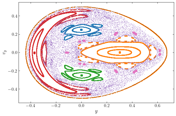
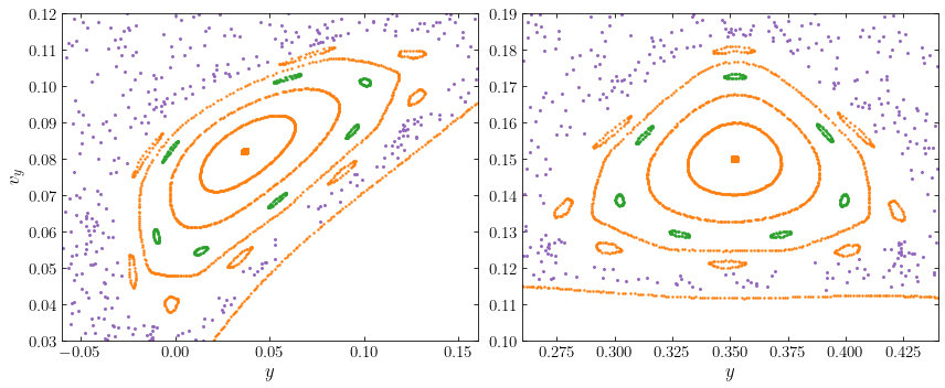
This surface of section looks very different from the one above. The same four stable orbit families are still present, but they are now embedded in a sea of purple points, all of which are points from a single orbit. This orbit does not follow a simple one-dimensional curve, but in fact fills an two-dimensional area. It therefore does not satisfy a second integral of the motion in addition to the energy and we have found a non-regular orbit (or a chaotic or ergodic orbit).

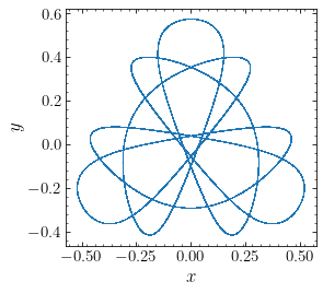
In addition to the chaotic orbit, the figure above also displays interesting structure around the stable orbit families. The stable orbit families themselves look similar to the orbit families at the \(E=1/12\) energy at which all orbits are regular: there are four closed parent orbits at the center of these families, indicated by the dots; these closed orbits look similar to those for \(E=1/12\) above. The boundaries of the orbit families no longer touch, but are now separated by the chaotic region. However, we see that there are small areas around the stable orbit families that the chaotic orbits do not enter. These are so-called islands, surrounding the main landmass of the stable orbit family. The loop-orbit families are surrounded by five islands, while the box-orbit families have four. The approximate edge of these islands are indicated with points with the same color as the main orbit family in the figure above. All islands surrounding a given family are visited by a single orbit: an orbit jumps between the different islands of the same color over the course of the orbit integration. The centers of the islands are higher-order closed orbits: they pierce through the surface of section at five (for the loop orbits) and four (for the box orbits) distinct points, located at the centers of the islands. For example, the orbit at the center of the orange islands is the following periodic orbit (this orbit is integrated for the same length of time as the chaotic orbit that fills much of the surface of section above!):

figsize(6,4)
E= 0.125
ts= numpy.linspace(0.,100000.,1000001)
o= orbit_yvyE(0.3525,0.15,E,pot=hp)
o.integrate(ts,hp)
o.plot(lw=0.25)
gca().set_aspect('equal');

The islands of the orange loop-orbit family above display further curious behavior, because the edge locus does not fully close. This is because we have in fact not found the actual edge of the island, but have instead landed on a higher-order set of islands. Let’s zoom in on two of the orange islands, the top-left and the top-middle one above:

figsize(12,5)
ys= [0.3025,0.3025,0.3025,0.3025,0.35,0.35,0.3525]
vys= [0.125,0.113,0.13,0.14,0.14,0.1325,0.15]
ts= numpy.linspace(0.,10000.,10000001)
for y,vy in zip(ys,vys):
    o= orbit_yvyE(y,vy,E,pot=hp)
    o.integrate(ts,hp)
    subplot(1,2,1)
    if vy == vys[-1]: marker=' o'
    else: marker= '.'
    sectys,sectvys=surface_section(o.x(ts),o.y(ts),o.vy(ts))
    if numpy.fabs(vy-0.14) < 0.001 \
        and numpy.fabs(y-0.3025) < 0.001: mfc= '#2ca02c'
    else: mfc= '#ff7f0e'
    plot(sectys,sectvys,marker,mec='none',zorder=2,mfc=mfc,ms=5.)
    subplot(1,2,2)
    plot(sectys,sectvys,marker,mec='none',zorder=2,mfc=mfc,ms=5.)
# Overplot chaotic trajectory from above
subplot(1,2,1)
xmin, xmax= -0.06,0.16
ymin, ymax= 0.03,0.12
# Need to use original times
ts= numpy.linspace(0.,100000.,10000001)
sectys,sectvys=surface_section(oc.x(ts),oc.y(ts),oc.vy(ts))
indx= (sectys > xmin)*(sectys < xmax)\
    *(sectvys > ymin)*(sectvys < ymax)
plot(sectys[indx],sectvys[indx],'.',mec='none',zorder=2,mfc='#9467bd')
xlabel(r'$y$')
ylabel(r'$v_y$')
xlim(xmin,xmax)
ylim(ymin,ymax)
subplot(1,2,2)
xmin, xmax= 0.26,0.44
ymin, ymax= 0.1,0.19
indx= (sectys > xmin)*(sectys < xmax)\
    *(sectvys > ymin)*(sectvys < ymax)
plot(sectys[indx],sectvys[indx],'.',mec='none',zorder=2,mfc='#9467bd')
xlabel(r'$y$')
xlim(xmin,xmax)
ylim(ymin,ymax)
tight_layout();

The lower orange edge is the edge of the main loop-orbit family above and the orange patches are the loci that are displayed in the full surface of section above; we have included some more curves closer to the center for each island as well. We see that in this zoomed-in version the loci near the edge of each island in the full surface of section turn out to be a family of eight islands themselves. These islands are second-order islands: they are islands of islands. At the center of these islands is another, more complicated, closed orbit. If we were to zoom in on these islands, we would find further hierarchies of islands. We have also found another set of islands inside of the main island; these are indicated in green and illustrate how ubiquitous islands are in the surface of section. The deep hierarchy of islands of ever decreasing size around islands that are themselves islands, etc., leads the chaos in the following way: as we go to orbits that are part of a set of islands that is very deep down in the hierarchy of islands, the orbit will appear to jump randomly between different parts of the surface of section and will appear to densely fill a two-dimensional area.

There is one more orbit shown in the full surface of section that is worth commenting on: the orbit that gives rise to the pink points. This orbit is a periodic orbit that appears to be deep in the chaotic regime. Any small perturbation to this orbit turns it into a chaotic orbit. For example, the following figure shows this period orbit over \(\Delta t = 10^5\) together with an orbit with a slightly lower initial \(y\):

figsize(14,6)
subplot(1,2,1)
ts= numpy.linspace(0.,100000.,3000001)
o= orbit_yvyE(-0.12,0.,E,pot=hp)
o.integrate(ts,hp)
o.plot(gcf=True,lw=0.5,xrange=[-0.7,0.7],yrange=[-0.55,0.75])
galpy_plot.text(r'$y_0=-0.120$',top_left=True,size=18.)
subplot(1,2,2)
# Integrate for same length, but get denser sampling
ts= numpy.linspace(0.,100000.,10000001)
o= orbit_yvyE(-0.125,0.,E,pot=hp)
o.integrate(ts,hp)
o.plot(gcf=True,marker=',',ls='none',alpha=0.005,rasterized=True,
       xrange=[-0.7,0.7],yrange=[-0.55,0.75])
galpy_plot.text(r'$y_0=-0.125$',top_left=True,size=18.)
tight_layout();

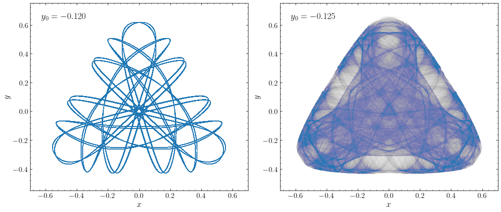
These orbits look very different: the periodic orbit remains well-behaved for long times, while the chaotic orbit fills all of the phase-space allowed by the conservation of energy (we have used transparency to more clearly display the projection of this orbit in \([x,y]\)).

The discussion in this section makes it clear that not all orbits in every two-dimensional non-axisymmetric potential have a second integral and consequently, that not all orbits in every three-dimensional axisymmetric potential satisfy a third integral. Some more realistic galactic potentials consisting of a disk and halo also have this property (e.g., Hunter 2005), although not all do. For some axisymmetric potentials all orbits are regular. An example of this is the Kuzmin potential that we discussed in Chapter 8.2.1. Such potentials are said to be integrable. Whether or not a galactic potential contains chaotic orbits and what fraction of the phase-space is chaotic is a question that needs to be answered for each potential separately.

It should be clear from this section how useful surfaces of section are in studying the importance of chaos in gravitational potentials. Because chaotic orbits fill a two-dimensional area in the surface of section, but do not enter regions of stability, the surface of section of a single chaotic orbit immediately delineates the chaotic and possibly-non-chaotic regions of phase space. For example, if we just plot the surface of section of the chaotic orbit at \(E=1/8\) from above we get the following:

figsize(9,6)
E= 1./8.
ts= numpy.linspace(0.,100000.,10000001)
sectys,sectvys=surface_section(oc.x(ts),oc.y(ts),oc.vy(ts))
plot(sectys,sectvys,',',mec='none',zorder=2,mfc='#9467bd')
# Also plot the zero-velocity curve
miny= optimize.brentq(lambda y: E-potential.evaluateplanarPotentials(hp,y,phi=numpy.pi/2.),
                     -0.45,-0.35)+1e-10
maxy= optimize.brentq(lambda y: E-potential.evaluateplanarPotentials(hp,y,phi=numpy.pi/2.),
                     0.6,0.8)-1e-10
ys= numpy.linspace(miny,maxy,201)
plot(ys,zvc(ys,E,pot=hp),color='k',zorder=10,lw=0.5)
plot(ys,-zvc(ys,E,pot=hp),color='k',zorder=11,lw=0.5)
xlabel(r'$y$')
ylabel(r'$v_y$');

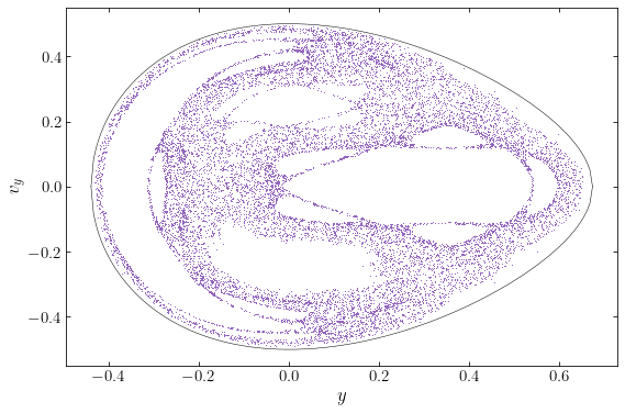
The chaotic orbit leaves many parts of the surface of section clear and we can identify the stable orbit families and the islands surrounding them directly. Of course, from this diagram we do not know whether the regions untouched by the chaotic orbits are regular or not, but we can investigate that by integrating orbits in each of these regions and determining their surface of section. Thus, the surface of section provides an easy way to investigate the orbital structure at a given energy.

14.4. Orbits in triaxial systems

\label{sec-triaxialorb-triaxialorb}

Unfortunately, in static triaxial potentials we cannot easily use surfaces of section, because static triaxial potentials only have a single classical integral of the motion (the specific energy) and this does not suffice to reduce the dimensionality of phase-space to three dimensions at a given energy. The study of orbits in triaxial systems is therefore far more difficult. However, there is also greater urgency in understanding the orbital structure of triaxial systems, because it is a priori not at all clear that static, long-term-stable triaxial mass configurations can be self-consistently constructed out of their orbits. That is, it is not clear that the density distribution obtained by letting a large number of bodies move along their orbits in a given triaxial gravitational potential can be the density that satisfies the Poisson equation for this potential for any setting of the relative number of bodies on different orbits.

The issue of whether or not a given mass distribution can be self-consistently constructed out of their orbits is not one that we have given much importance to up until now. We discussed equilibrium configurations of spherical systems in Chapter 6, where we derived the Eddington formula for determining the ergodic (isotropic) distribution function that self-consistently generates the density in Section 6.6.1. We saw there that it is possible for this ergodic distribution function to be negative, meaning that there isn’t a self-consistent ergodic distribution function for all spherical systems. But once we relax the requirement of isotropy, it is clear that there is always an anisotropic distribution function that can self-consistently generate a given spherical density: we can simply build the density with shells made up of bodies on circular orbits, with the number of bodies proportional to the surface density of each shell. Similarly, we did not consider self-consistency much when discussing distributions of orbits in disk in Chapter 11 for two reasons. First of all, galactic disks are embedded in massive dark-matter halos and the disk therefore only ever contributes part of the gravitating mass density (albeit a not-insubstantial part). Second of all, as for spherical systems, we can build razor-thin disk distributions out of circular orbits with the number of bodies on each orbit set to match the disk’s surface density (e.g., Section 11.2.1) and it is quite plausible that we can generate any realistic warm, thick disk by heating such a cold distribution function in the radial and vertical direction (e.g., Sections 11.2.2 and 11.4). Thus, it is clear that spherical and axisymmetric disky systems can be relatively-easily self-consistently generated (although we will side-step the question of whether such configurations are stable, which especially for disks can be an issue).

Whether or not triaxial configurations can be self-consistently generated is not immediately clear. The obvious generalization of the existence “proof” of self-consistent solutions for spherical and disk systems from the previous paragraph is to build a self-consistent solution out of the generalizations of circular orbits. As we saw in Section 14.2 above, in two-dimensional non-axisymmetric systems (an easy toy stand-in for full three-dimensional triaxial systems that we will rely on further below), generalized circular orbits are the closed loop orbits. But let’s see what happens when we look at a closed loop orbit in, for example, the non-axisymmetric logarithmic potential that we employed in Section 14.2 above:

from galpy.potential import LogarithmicHaloPotential
from galpy.orbit import Orbit
lp= LogarithmicHaloPotential(normalize=True,b=0.8,core=0.2)
ts= numpy.linspace(0.,10.,601)
figsize(5,5)
lp.plotSurfaceDensity(xmin=-0.43,xmax=0.43,ymin=-0.43,ymax=0.43,justcontours=True,log=True,ncontours=5)
o= Orbit([0.147,0.,1.07630163,0.])
o.integrate(ts,lp)
o.plot(gcf=True,lw=2.)
o= Orbit([0.147,0.15,1.07630163,0.])
o.integrate(ts,lp)
o.plot(gcf=True,zorder=0)
xlim(-0.43,0.43)
ylim(-0.43,0.43)
gca().set_aspect('equal');

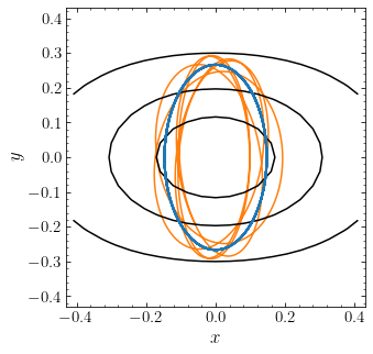
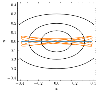
The closed loop orbit is shown as the solid curve elongated in the \(y\) direction and we have also drawn three contours of constant (surface) density. From this we see that the closed loop orbit is elongated in the direction perpendicular to the direction along which the density is elongated! This remains the case if we go to non-closed loop orbits (the non-closed orbit elongated in the \(y\) direction in the figure above) and it is generally true for loop orbits in non-axisymmetric potentials. Because they are elongated in the wrong direction, loop orbits cannot be a significant contributor to the density of self-consistent non-axisymmetric systems. Instead, box orbits need to contain a substantial fraction of the mass, because they are elongated in the correct direction. For example, a closed and non-closed box orbit with a similar energy as the loop orbits above look as follows:

from galpy.potential import LogarithmicHaloPotential
from galpy.orbit import Orbit
lp= LogarithmicHaloPotential(normalize=True,b=0.8,core=0.2)
figsize(5,5)
lp.plotSurfaceDensity(xmin=-0.43,xmax=0.43,ymin=-0.43,ymax=0.43,justcontours=True,log=True,ncontours=5)
o= Orbit([0.147,1.07630163,0.,0.])
o.integrate(ts,lp)
o.plot(gcf=True,lw=2.)
o= Orbit([0.147,1.07630163,0.2,0.])
o.integrate(ts,lp)
o.plot(gcf=True,zorder=0)
xlim(-0.43,0.43)
ylim(-0.43,0.43)
gca().set_aspect('equal');

Thus, box orbits are crucial for building triaxial mass distributions and whether or not a long-term stable, self-consistent triaxial density is possible therefore depends on whether or not box orbits exist and are stable.

In this section, we therefore discuss the properties of orbits in three-dimensional triaxial systems in detail with special attention focused on the box orbits. We start by discussing the major orbit families in triaxial systems, which will turn out to be box orbits and different generalizations of the loop orbits. Then we will move on to a more in-depth discussion of when box orbits exist, how they may be destroyed, and whether they can exist in realistic models for elliptical galaxies and dark matter halos.

14.4.1. The major orbit families in triaxial gravitational potentials: orbits in the perfect ellipsoid

\label{sec-triaxialorbit-majororbs}

Visualizing and studying orbits in six-dimensional phase-space is difficult and in the previous parts, we made use of the fact that spherical and axisymmetric systems are separable in various ways to simplify the investigation of their orbits. For example, the conservation of the magnitude and direction of the angular momentum in spherical systems means that overall properties of their orbits can be studied as the dynamics in a one-dimensional effective potential (see Chapter 5.1) . Similarly, the conservation of the \(z\) component of the angular momentum in axisymmetric systems means that we can study their orbits in the \((R,z)\) meridional plane (Chapter 10.1). Furthermore, for orbits that remain close to the mid-plane in a disk potential, the \(R\) and \(z\) motions separate approximately, further simplifying their dynamics (Chapter 10.2) and allowing us to make simple steady-state models for disks (see Chapter 11).

Being able to separate the full six-dimensional dynamics of a gravitational system into lower-dimensional components is therefore highly useful. Unfortunately, the lack of symmetries in static triaxial mass distributions beyond the time invariance that leads to energy conservation, means that orbits in triaxial systems cannot in general be simplified by separating components. The exception to this rule are the Staeckel potentials. These are the most general class of potentials for which the Hamilton-Jacobi equation from Chapter 4.4.3 can be solved using the separation-of-variables technique. As discussed in Chapter 4.4.3, if the Hamilton-Jacobi equation can be separated, then orbits are regular (i.e., not chaotic) and are fully described as the combination of three independent oscillations in a two-dimensional phase-space each. The most general coordinate system in which the Hamilton-Jacobi equation can be solved using the separation-of-variables technique is that of ellipsoidal coordinates, a generalization of the oblate and prolate spheroidal coordinates that we discussed in Chapter 13.2.1. Ellipsoidal coordinates \((\lambda,\mu,\nu)\) for a given cartesian point \((x,y,z)\) are defined as the three roots of the equation

\begin{equation}\label{eq-triaxialorbs-ellipsoidal-coords-definition} {x^2 \over \tau + \alpha} + {y^2 \over \tau + \beta} +{z^2 \over \tau + \gamma} = 1\,, \end{equation}

where \((\alpha,\beta,\gamma)\) are constants that define the coordinate system that satisfy \(\alpha < \beta < \gamma\). We further order the roots such that \(\nu < \mu < \lambda\); the roots then satisfy

\begin{equation} -\gamma \leq \nu \leq -\beta \leq \mu \leq -\alpha \leq \lambda\,. \end{equation}

Because \(\lambda\), \(\mu\), and \(\nu\) cover different ranges, in many situations we can also represent them using a single variable \(\tau\) that either denotes \(\lambda\), \(\mu\), or \(\nu\) depending on which range it falls in. For completeness, we note that the inverse transformation from ellipsoidal to cartesian coordinates is given by

\begin{align} x^2 & = {(\lambda + \alpha)(\mu + \alpha)(\nu + \alpha) \over (\alpha-\beta)(\alpha-\gamma)}\,,\\ y^2 & = {(\lambda + \beta)(\mu + \beta)(\nu + \beta) \over (\beta-\alpha)(\beta-\gamma)}\,,\\ z^2 & = {(\lambda + \gamma)(\mu + \gamma)(\nu + \gamma) \over (\gamma-\alpha)(\gamma-\beta)}\,. \end{align}

Each of \((x,y,z)\) is therefore only specified up to a sign. The transformation equations for the momenta can be derived using the coordinate-transformation generation function from Chapter 4.4.2. Staeckel potentials are then potentials that in ellipsoidal coordinates can be written as

\begin{equation}\label{eq-triaxialorbs-staeckel} \Phi(\lambda,\mu,\nu) = {f(\lambda) \over (\lambda-\mu)(\nu-\lambda)} + {f(\mu) \over (\mu-\nu)(\lambda-\mu)} + {f(\nu) \over (\nu-\lambda)(\mu-\nu)} \,. \end{equation}

For this form of the potential, the Hamilton-Jacobi equation in ellipsoidal coordinates can be solved by separating the variables.

Few galactic potentials can be written in the form of Equation \eqref{eq-triaxialorbs-staeckel} in any ellipsoidal coordinate system, but one example is the perfect ellipsoid that we introduced in Chapter 13.2.3. In fact, the perfect ellipsoid is the only gravitational potential of Staeckel form for which the density is stratified on similar ellipsoids (\(\rho\equiv \rho(m)\) for \(m\) given by Equation 13.45; de Zeeuw & Lynden-Bell 1985). Thus, it is the only realistic triaxial galactic potential for which the Hamilton-Jacobi equation can be solved using the separation-of-variables technique and where orbits, therefore, can be easily studied by separating them into lower-dimensional components. As such, the perfect ellipsoid is the perfect potential to learn about the major orbit families that exist in triaxial galactic mass distributions!

More specifically, the perfect ellipsoid potential for a given set of axis lengths \(a > b > c\) can be written in Staeckel form when we set \(\alpha = -a^2\), \(\beta = -b^2\), and \(\gamma = -c^2\). Because the orbits separate into decoupled motions in \(\lambda\), \(\mu\), and \(\nu\), we can get a first sense of the orbital structure by considering what surfaces with constant values of one of these coordinates look like: orbits oscillate between such surfaces. For this, we first implement the transformation between cartesian and ellipsoidal coordinates:

def cartesian_to_ellipsoidal(x,y,z,alpha,beta,gamma):
    x= numpy.atleast_1d(x)
    y= numpy.atleast_1d(y)
    z= numpy.atleast_1d(z)
    N= len(x)
    out= numpy.empty((N,3))
    for ii,(tx,ty,tz) in enumerate(zip(x,y,z)):
        these_coords= numpy.polynomial.polynomial.Polynomial(\
                        (beta*gamma*tx**2.+alpha*gamma*ty**2.+alpha*beta*tz**2.
                         -alpha*beta*gamma,
                        (beta+gamma)*tx**2.+(alpha+gamma)*ty**2.+(alpha+beta)*tz**2.
                         -alpha*beta-alpha*gamma-beta*gamma,
                        tx**2.+ty**2.+tz**2.-alpha-beta-gamma,
                        -1.)).roots()
        out[ii]= sorted(these_coords)[::-1]
    return out
def ellipsoidal_to_cartesian(l,m,n,alpha,beta,gamma):
    x= numpy.sqrt((l+alpha)*(m+alpha)*(n+alpha)/(alpha-beta)/(alpha-gamma))
    y= numpy.sqrt((l+beta)*(m+beta)*(n+beta)/(beta-alpha)/(beta-gamma))
    z= numpy.sqrt((l+gamma)*(m+gamma)*(n+gamma)/(gamma-beta)/(gamma-alpha))
    return numpy.array([x,y,z]).T

Then we can look at surfaces of constant \(\lambda\), \(\mu\), and \(\nu\) for a potential with \(a = 1\), \(b = 0.7\), and \(c = 0.5\):

from scipy import interpolate
from mpl_toolkits.mplot3d import Axes3D
from matplotlib import cm
from matplotlib.colors import Normalize
def draw_coordinate_axes(ax,size=2.5):
    # Draw centered axes (https://stackoverflow.com/a/61927456)
    val = [size,0,0]
    labels = [r'$x$', r'$y$', r'$z$']
    for v in range(3):
        x = [val[v-0], -val[v-0]]
        y = [val[v-1], -val[v-1]]
        z = [val[v-2], -val[v-2]]
        ax.plot(x,y,z,'k-', linewidth=1)
        ax.text(val[v-0]-0.1,val[v-1],val[v-2]-0.25,
                labels[v],color='k',fontsize=20)
    return None
a, b, c= 1., 0.7, 0.5
alpha, beta, gamma= -a**2., -b**2., -c**2.
fig= plt.figure(figsize=[16.,4.8])
ax= fig.add_subplot(1,3,1,projection='3d')
# Surface of constant lambda
la,_,_= cartesian_to_ellipsoidal(1.,0.,0.,alpha,beta,gamma).T
mus= numpy.linspace(-beta,-alpha,11)
nus= numpy.linspace(-gamma,-beta,11)
munus= numpy.meshgrid(mus,nus,indexing='ij')
xyz= ellipsoidal_to_cartesian(la[0]+numpy.zeros_like(munus[0]),
                              munus[0],munus[1],alpha,beta,gamma)
norm= Normalize(-numpy.nanmax(xyz[:,:,2]),numpy.nanmax(xyz[:,:,2]))
for sgnx in [-1,1]:
    for sgny in [-1,1]:
        for sgnz in [-1,1]:
            ax.plot_trisurf(sgnx*xyz[:,:,0].flatten(),
                            sgny*xyz[:,:,1].flatten(),
                            sgnz*xyz[:,:,2].flatten(),
                            cmap=cm.plasma,norm=norm,
                            linewidth=10.2,antialiased=True)
draw_coordinate_axes(ax,size=2.5)
ax.view_init(40,50)
ax.set_xlim(-1.2,1.2)
ax.set_ylim(-1.2,1.2)
ax.set_zlim(-1.2,1.2)
ax._axis3don= False
annotate(r'$\mathrm{constant}\ \lambda$',
         (0.5,0.05),xycoords='axes fraction',
         horizontalalignment='center',size=28.)
ax= fig.add_subplot(1,3,2,projection='3d')
# Surface of constant mu
_,ma,_= cartesian_to_ellipsoidal(0.3,0.4,0.3,alpha,beta,gamma).T
las= numpy.linspace(-alpha,-alpha+3.,11)
nus= numpy.linspace(-gamma,-beta,11)
lanus= numpy.meshgrid(las,nus,indexing='ij')
xyz= ellipsoidal_to_cartesian(lanus[0],ma[0]+numpy.zeros_like(lanus[0]),
                              lanus[1],alpha,beta,gamma)
norm= Normalize(-numpy.nanmax(xyz[:,:,2]),numpy.nanmax(xyz[:,:,2]))
for sgnx in [-1,1]:
    for sgny in [-1,1]:
        for sgnz in [-1,1]:
            ax.plot_trisurf(sgnx*xyz[:,:,0].flatten(),
                            sgny*xyz[:,:,1].flatten(),
                            sgnz*xyz[:,:,2].flatten(),
                            cmap=cm.plasma,norm=norm,
                            linewidth=10.2,antialiased=True)
draw_coordinate_axes(ax,size=2.5)
ax.view_init(40,50)
ax.set_xlim(-1.2,1.2)
ax.set_ylim(-1.2,1.2)
ax.set_zlim(-1.2,1.2)
ax._axis3don= False
annotate(r'$\mathrm{constant}\ \mu$',
         (0.5,0.05),xycoords='axes fraction',
         horizontalalignment='center',size=28.)
ax= fig.add_subplot(1,3,3,projection='3d')
# Surface of constant nu
_,_,na= cartesian_to_ellipsoidal(0.5,0.6,0.7,alpha,beta,gamma).T
las= numpy.linspace(-alpha,-alpha+2.,11)
mus= numpy.linspace(-beta,-alpha,11)
lamus= numpy.meshgrid(las,mus,indexing='ij')
xyz= ellipsoidal_to_cartesian(lamus[0],lamus[1],
                              na[0]+numpy.zeros_like(lamus[0]),alpha,beta,gamma)
norm= Normalize(-numpy.nanmax(xyz[:,:,2]),numpy.nanmax(xyz[:,:,2]))
for sgnx in [-1,1]:
    for sgny in [-1,1]:
        for sgnz in [-1,1]:
            ax.plot_trisurf(sgnx*xyz[:,:,0].flatten(),
                            sgny*xyz[:,:,1].flatten(),
                            sgnz*xyz[:,:,2].flatten(),
                            cmap=cm.plasma,norm=norm,
                            linewidth=10.2,antialiased=True)
draw_coordinate_axes(ax,size=2.5)
ax.view_init(40,50)
ax.set_xlim(-1.2,1.2)
ax.set_ylim(-1.2,1.2)
ax.set_zlim(-1.2,1.2)
ax._axis3don= False
annotate(r'$\mathrm{constant}\ \nu$',
         (0.5,0.05),xycoords='axes fraction',
         horizontalalignment='center',size=28.);

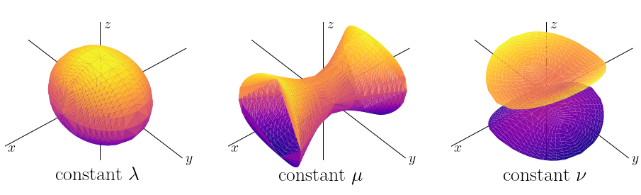
Surfaces of constant \(\lambda\) are ellipsoids with the long axis in the \(z\) direction and the short axis in the \(x\) direction. For \(\lambda \gg -\alpha\), these ellipsoids are approximately spherical, while for \(\lambda = -\alpha\), the ellipsoid collapses to a 2D ellipse at \(x=0\). Surface of constant \(\mu\) are hyperboloids of one sheet and surfaces of constant \(\nu\) are hyperbolae of two sheets. The one-sheet hyperboloids collapse to a 2D hyperbola at \(y=0\) for \(\mu = -\beta\), while the two-sheet hyperboloid collapses to a two-dimensional area at \(z=0\). At small distances from the origin, the ellipsoidal coordinate system is approximately the cartesian, while at large distances it is approximately spherical; the ellipsoidal coordinate system therefore smoothly interpolates between these two extremes. This is similar to how the oblate and prolate coordinate systems that we used in Chapter 13.2.1 go from being approximately the cylindrical coordinate frame at small distances from the origin to being approximately spherical at large distances.

Because of the separability of the Hamilton-Jacobi equation for the perfect ellipsoid, one can compute two integrals of the motion in addition to the specific energy that are generalizations of the \(z\)-component of the angular momentum and the third integral for axisymmetric systems; we denote these as \(I_2\) and \(I_3\). Similar to what is possible for spherical and axisymmetric systems, the motion in the perfect ellipsoid can be described as that in a one-dimensional effective potential \(\Phi_{\mathrm{eff}}(\tau)\) for a given value of \(I_2\) and \(I_3\) (where we write this potential as a function of \(\tau\) to cover all three coordinates as explained above). It turns out that motion is then possible in regions where \(\Phi_{\mathrm{eff}}(\lambda) \leq E\), \(\Phi_{\mathrm{eff}}(\mu) \leq E\), and \(\Phi_{\mathrm{eff}}(\nu) \geq E\); note that the inequality in the last equation is opposite that of the others (and opposite to the equivalent condition for spherical or axisymmetric systems). Turning points of the orbit are then those \(\tau\) where \(\Phi_{\mathrm{eff}}(\tau) = E\) and this equation is satisfied for all orbits at three points \(\tau_i\) (up from two in the spherical and axisymmetric case). Depending on where the \(\tau_i\) lie relative to \(-\gamma\), \(-\beta\), and \(-\alpha\), we get different types of orbits.

From Equation \eqref{eq-triaxialorbs-ellipsoidal-coords-definition} it is clear that the origin \((x,y,z) = (0,0,0)\) is mapped onto \((\lambda,\mu,\nu) = (-\alpha,-\beta,-\gamma)\). Orbits with the three turning points \(\tau_i\) arranged as \(-\gamma < \tau_1 < -\beta < \tau_2 < -\alpha < \tau_3\) are therefore able to pass through the origin. In each ellipsoidal coordinate direction, they oscillate between the two-dimensional area at \(x,y,z=0\) at \(\lambda,\mu,\nu = -\alpha,-\beta,-\gamma\) and the ellipsoid or hyperboloid of their turning point. The three-dimensional volume is therefore a box and these are the three dimensional box orbits. It turns out that there are three other possible arrangements of the turning points and they all have two turning points either between \(-\beta\) and \(-\alpha\) or above \(-\alpha\). Such orbits do not include \((\lambda,\mu,\nu) = (-\alpha,-\beta,-\gamma)\) and therefore do not pass through the origin. These orbits have a definite sense of rotation around one of the axes and are the generalizations of the loop orbits in axisymmetric potentials; in the context of triaxial systems they are known as tube orbits. Orbits with \(-\gamma < \tau_1 < -\beta < -\alpha < \tau_2 < \tau_3\) oscillate between two ellipsoids in \(\lambda\) and between the two branches of the turning hyperboloid of two sheets corresponding to \(\tau_1\). From the constant \(\nu\) and constant \(\lambda\) shapes in the figure above, it is clear that such orbits loop around the minor, \(z\) axis. These orbits are known as the short-axis tube orbits. The remaining two options both have one or two turning hyperboloids of one sheet, which avoid the \(x\) axis and these orbits therefore loop around the major, \(x\) axis; they are known as long-axis tube orbits. They further separate into two classes depending on whether there are one or two turning hyperboloids of one sheet: \(-\gamma < -\beta < \tau_1 < \tau_2 < -\alpha < \tau_3\) is an inner long-axis tube orbit, while \(-\gamma < -\beta < \tau_1 < -\alpha < \tau_2 < \tau_3\) gives an outer long-axis tube orbit. The following figure displays a representative example of these four orbit families:

from galpy.potential import PerfectEllipsoidPotential
from galpy.orbit import Orbit
from mpl_toolkits.mplot3d import Axes3D
def draw_coordinate_axes(ax,size=2.5,shrinkx=1.,shrinkz=1.):
    # Draw centered axes (https://stackoverflow.com/a/61927456)
    val = [size,0,0]
    labels = [r'$x$', r'$y$', r'$z$']
    for v in range(3):
        x = [val[v-0]/shrinkx,-val[v-0]/shrinkx]
        y = [val[v-1],-val[v-1]]
        z = [val[v-2]/shrinkz, -val[v-2]/shrinkz]
        ax.plot(x,y,z,'k-',linewidth=1)
        ax.text(val[v-0]/shrinkx-0.1/shrinkx,
                val[v-1],val[v-2]/shrinkz-0.25/shrinkz,
                labels[v],color='k',fontsize=20)
    return None
a, b, c= 1., 0.7, 0.5
pep= PerfectEllipsoidPotential(normalize=1.,a=a,b=b,c=c)
fig= plt.figure(figsize=[10.,10])
ax= fig.add_subplot(2,2,1,projection='3d')
# box orbit
o= Orbit([0.5,-0.01,0.991,0.15,0.,numpy.pi/2.])
ts= numpy.linspace(0.,10000.,100001)
o.integrate(ts,pep)
ax.scatter(o.x(ts),o.y(ts),o.z(ts),marker='o',
           s=5.,edgecolors=None,alpha=0.01)
ax.view_init(40,50.)
ax.set_xlim(-1.,1.)
ax.set_ylim(-1.,1.)
ax.set_zlim(-0.25,0.25)
ax._axis3don= False
draw_coordinate_axes(ax,size=1.5,shrinkz=2.50)
annotate(r'$\mathrm{box}$',
             (0.5,0.05),xycoords='axes fraction',
             horizontalalignment='center',size=28.)
# Short axis tube
ax= fig.add_subplot(2,2,2,projection='3d')
o= Orbit([1.2,-0.21,0.61,0.4,-0.2,numpy.pi/2.])
ts= numpy.linspace(0.,10000.,100001)
o.integrate(ts,pep)
ax.scatter(o.x(ts),o.y(ts),o.z(ts),marker='o',
           s=5.,edgecolors=None,alpha=0.01)
ax.view_init(40,50.)
ax.set_xlim(-1.,1.)
ax.set_ylim(-1.,1.)
ax.set_zlim(-.6,.6)
ax._axis3don= False
draw_coordinate_axes(ax,size=1.85,shrinkz=1.25)
annotate(r'$\mathrm{short-axis\ tube}$',
             (0.5,0.05),xycoords='axes fraction',
             horizontalalignment='center',size=28.)
# Inner long-axis tube orbit
ax= fig.add_subplot(2,2,3,projection='3d')
o= Orbit([0.4,0.51,0.51,.6,-0.195,0.])
ts= numpy.linspace(0.,2000.,100001)
o.integrate(ts,pep)
ax.scatter(o.x(ts)*1.25,o.y(ts)*1.25,o.z(ts)*1.25,
           marker='o',s=8.,edgecolors=None,alpha=0.01)
ax.view_init(20,40)
ax.set_xlim(-.75,.75)
ax.set_ylim(-1.,1.)
ax.set_zlim(-1.,1.)
ax._axis3don = False
draw_coordinate_axes(ax,size=1.65)
annotate(r'$\mathrm{inner\ long-axis\ tube}$',
             (0.5,0.05),xycoords='axes fraction',
             horizontalalignment='center',size=28.)
# Outer long-axis tube orbit
ax= fig.add_subplot(2,2,4,projection='3d')
o= Orbit([2.9,0.31,0.41,2.4,-0.675,numpy.pi/2.])
ts= numpy.linspace(0.,10000.,100001)
o.integrate(ts,pep)
ax.scatter(o.x(ts)/4.,o.y(ts)/4.,o.z(ts)/4.,
           marker='o',s=5.,edgecolors=None,alpha=0.01)
ax.view_init(20,30.)
ax.set_xlim(-1.,1.)
ax.set_ylim(-1.,1.)
ax.set_zlim(-1.,1.)
ax._axis3don = False
draw_coordinate_axes(ax,size=1.6,shrinkx=0.8)
annotate(r'$\mathrm{outer\ long-axis\ tube}$',
             (0.5,0.05),xycoords='axes fraction',
             horizontalalignment='center',size=28.)
tight_layout();

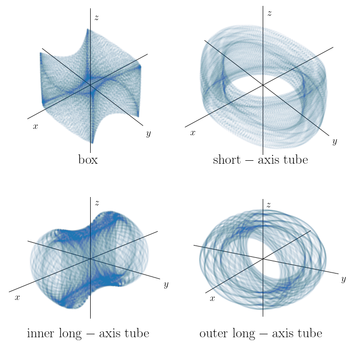
These four orbit families constitute the main orbit families in all triaxial mass distributions. The box orbits and the short-axis tube orbits are the generalizations of the box and loop orbits in two-dimensional, non-axisymmetric potentials that we saw in Section 14.2 above and those loop orbits were themselves the generalizations of the loop orbits in axisymmetric mass distributions. However, there is no analog of the long-axis tube orbits in axisymmetric systems and these orbits only exist as stable orbit families in triaxial mass distributions. Observationally, these manifest themselves as apparent rotation along the minor axis and this minor-axis rotation is therefore a tell-tale observational signature of triaxiality (see the discussion in Chapter 13.1). That there is no intermediate-axis tube orbit family means that there are no stable orbits that loop around the intermediate axis (Heiligman & Schwarzschild 1979).

As an example of these four main orbit families in other triaxial potentials, we can look at similar orbits as those shown above, but now computed in a triaxial NFW potential:

from galpy.potential import TriaxialNFWPotential
from galpy.orbit import Orbit
from mpl_toolkits.mplot3d import Axes3D
def draw_coordinate_axes(ax,size=2.5,shrinkx=1.,shrinkz=1.):
    # Draw centered axes (https://stackoverflow.com/a/61927456)
    val = [size,0,0]
    labels = [r'$x$', r'$y$', r'$z$']
    for v in range(3):
        x = [val[v-0]/shrinkx,-val[v-0]/shrinkx]
        y = [val[v-1],-val[v-1]]
        z = [val[v-2]/shrinkz, -val[v-2]/shrinkz]
        ax.plot(x,y,z,'k-',linewidth=1)
        ax.text(val[v-0]/shrinkx-0.1/shrinkx,
                val[v-1],val[v-2]/shrinkz-0.25/shrinkz,
                labels[v],color='k',fontsize=20)
    return None
a, b, c= 1., 0.7, 0.5
nep= TriaxialNFWPotential(normalize=1.,a=a,b=b,c=c)
fig= plt.figure(figsize=[10.,10])
ax= fig.add_subplot(2,2,1,projection='3d')
# box orbit
o= Orbit([0.1,-0.7,0.9,0.15,0.,numpy.pi/2.])
ts= numpy.linspace(0.,10000.,100001)
o.integrate(ts,nep,method='dop853_c')
ax.scatter(o.x(ts)*2,o.y(ts)*2,o.z(ts)*2,marker='o',
           s=5.,edgecolors=None,alpha=0.01)
ax.view_init(40,50.)
ax.set_xlim(-1.,1.)
ax.set_ylim(-1.,1.)
ax.set_zlim(-1.,1.)
ax._axis3don= False
draw_coordinate_axes(ax,size=1.5,shrinkz=0.8)
annotate(r'$\mathrm{box}$',
             (0.5,0.05),xycoords='axes fraction',
             horizontalalignment='center',size=28.)
# Short axis tube
ax= fig.add_subplot(2,2,2,projection='3d')
o= Orbit([1.2,-0.21,0.61,0.4,-0.2,numpy.pi/2.])
ts= numpy.linspace(0.,10000.,100001)
o.integrate(ts,nep,method='dop853_c')
ax.scatter(o.x(ts),o.y(ts),o.z(ts),marker='o',
           s=5.,edgecolors=None,alpha=0.01)
ax.view_init(40,50.)
ax.set_xlim(-1.,1.)
ax.set_ylim(-1.,1.)
ax.set_zlim(-.6,.6)
ax._axis3don= False
draw_coordinate_axes(ax,size=1.85,shrinkz=1.25)
annotate(r'$\mathrm{short-axis\ tube}$',
             (0.5,0.05),xycoords='axes fraction',
             horizontalalignment='center',size=28.)
# Inner long-axis tube orbit
ax= fig.add_subplot(2,2,3,projection='3d')
o= Orbit([0.4,0.51,0.51,.6,-0.195,0.])
ts= numpy.linspace(0.,2000.,100001)
o.integrate(ts,nep,method='dop853_c')
ax.scatter(o.x(ts)*1.25,o.y(ts)*1.25,o.z(ts)*1.25,
           marker='o',s=8.,edgecolors=None,alpha=0.01)
ax.view_init(20,40)
ax.set_xlim(-.75,.75)
ax.set_ylim(-1.,1.)
ax.set_zlim(-1.,1.)
ax._axis3don = False
draw_coordinate_axes(ax,size=1.65)
annotate(r'$\mathrm{inner\ long-axis\ tube}$',
             (0.5,0.05),xycoords='axes fraction',
             horizontalalignment='center',size=28.)
# Outer long-axis tube orbit
ax= fig.add_subplot(2,2,4,projection='3d')
o= Orbit([2.9,0.31,0.41,2.4,-0.675,numpy.pi/2.])
ts= numpy.linspace(0.,10000.,100001)
o.integrate(ts,nep,method='dop853_c')
ax.scatter(o.x(ts)/4.,o.y(ts)/4.,o.z(ts)/4.,marker='o',
           s=5.,edgecolors=None,alpha=0.01)
ax.view_init(20,30.)
ax.set_xlim(-1.,1.)
ax.set_ylim(-1.,1.)
ax.set_zlim(-1.,1.)
ax._axis3don = False
draw_coordinate_axes(ax,size=1.6,shrinkx=0.8)
annotate(r'$\mathrm{outer\ long-axis\ tube}$',
             (0.5,0.05),xycoords='axes fraction',
             horizontalalignment='center',size=28.)
tight_layout();

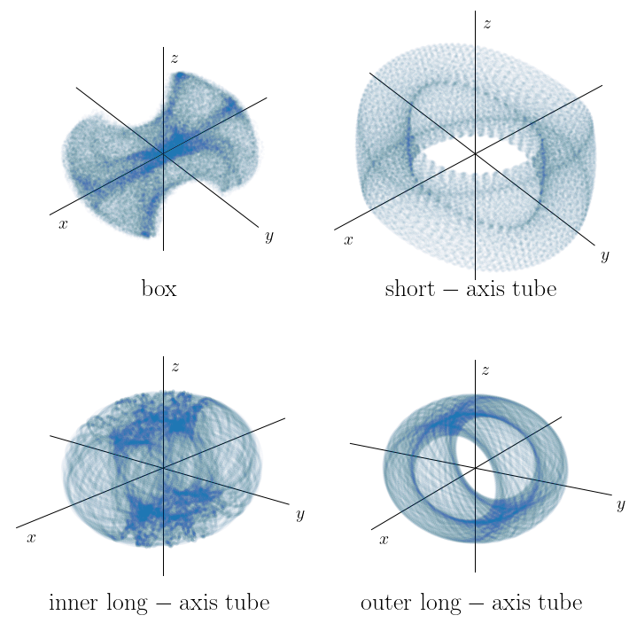
We see that these orbits are qualitatively similar to those in the perfect ellipsoid and the main orbit families are therefore the same in a triaxial NFW potential as in the perfect ellipsoid. But the two orbit families that approach the center the closest—the box orbits and the inner long-axis tubes—look somewhat different. This is because the inner density of the NFW potential is very different from that of the perfect ellipsoid: the perfect ellipsoid has a constant-density core at \(m \ll 1\), while the NFW density diverges as \(\rho(m) \propto m^{-1}\). We see in particular that the box orbit is more concentrated towards the center and more fanned out at large distances than a similar box orbit in the perfect ellipsoid. Because box orbits are so important for building self-consistent models of triaxial mass distributions, this spells trouble.

14.4.2. Orbits in non-axisymmetric potentials with central density cusps

\label{sec-triaxialorbs-nonaxi-cuspy}

As we discussed in Chapter 13.1, elliptical galaxies have inner surface-density profiles that are power-laws: \(I(R) \propto R^{-\gamma}\) with \(0 < \gamma \lesssim 1\). In particular, the surface density keeps increasing at the smallest scale that can be resolved in all elliptical galaxies, albeit very shallowly in luminous elliptical galaxies (\(0 < \gamma \lesssim 0.3\)). Thus, unlike the perfect ellipsoid or the two-dimensional cored logarithmic potential from Section 14.2 above, elliptical galaxies have cuspy rather than cored profiles. The same holds for dark-matter halos, where \(\rho(r) \propto r^{-1}\) (Section 3.4.6). However, we derived the existence of box orbits in Section 14.2 from the approximately-harmonic motion that occurs in a constant-density mass distribution. If the gravitational potential is not harmonic however close we get to the center, it is therefore not clear that box orbits exist or are long-term stable.

Another reason that elliptical galaxies have a central non-harmonic potential is the existence of supermassive black holes at their centers (we will discuss the evidence for this further in Chapter 17.1). The presence of a supermassive black hole has various dynamical consequences. The most obvious is that the black hole constitutes a point-mass potential and that the motion near the black hole is therefore Keplerian rather than harmonic. Stars that orbit within the region where the black hole dominates the mass distribution—the black hole’s so called sphere of influence, which is about \(5\) to \(50\,\mathrm{pc}\) depending on its mass—are therefore Keplerian ellipses rather than box orbits. But the larger-scale orbital distribution is also affected by the supermassive black hole, because any box orbit eventually enters the black hole’s sphere of influence on a hyperbolic trajectory and exits it on a different orbit due to the deflection from the interaction with the black hole. This tends to disrupt the skinny box orbits that are crucial for building triaxial systems. A secondary effect occurs when the black hole grows smoothly: then it is predicted to adiabatically grow a steep cusp of stars with \(\rho(r) \propto r^{-7/4}\) (Bahcall & Wolf 1976) that further pushes the potential away from harmonicity (however, no such cusps have ever been observed). Numerical studies of orbits in two-dimensional (e.g., Gerhard & Binney 1985) and three-dimensional non-axisymmetric mass distributions (e.g., Merritt & Valluri 1996; Merritt & Quinlan 1998; Valluri & Merritt 1998) demonstrate that supermassive black holes with masses exceeding \(\approx 0.5\,\%\) of the galaxy’s mass significantly disrupt the box orbits even in an otherwise cored gravitational potential. However, enough box orbits survive such that combined with weakly-chaotic orbits they can support the global triaxiality of such models even when the black hole is as massive as \(1\,\%\) of the galaxy’s mass (Holley-Bockelmann et al. 2002). Because supermassive black holes typically have masses of \(\approx 0.2\) to \(0.3\,\%\) of the galaxy’s mass (e.g., Magorrian et al. 1998; Häring & Rix 2004; Gültekin et al. 2009), orbital evolution induced by them is therefore likely not that important, at least on scales beyond the inner tens of parsecs where the black hole dominates the gravitational potential. We leave a more detailed exploration of this topic therefore to the exercises and focus here on the effecct of density cusps.

The density cusps we are interested in behave as \(\rho(r) \propto r^{-\gamma}\) with \(\gamma \approx 1\) for dark-matter halos (see Chapter 3.4.6), and \(0 \lesssim \gamma \lesssim 1\) or \(1 \lesssim \gamma \lesssim 2\) for the shallow or steep cusps at the centers of luminous and less luminous elliptical galaxies (see Chapter 13.1). From the behavior of spherical power-law density profiles that we discussed in Chapter 3.4.5, it is clear that the force at the origin is finite for \(\gamma \leq 1\), while it diverges for \(\gamma > 1\). While the force diverges, the circular velocity remains finite until \(\gamma > 2\); this indicates that while the central force may diverge, the orbital it gives rise to are limited. At \(\gamma > 2\), both the central force and the circular velocity diverge and orbits that pass near the center are strongly affected by the central cusp. Therefore, there are three important regimes (Gerhard & Binney 1985):

• \(\gamma \leq 1\) (\(\rho[r]\) shallower than \(1/r\)): a density cusps exists, but the central force and circular velocity remain finite. In a triaxial system, the dynamics is therefore not qualitatively different from that in a constant-density core and we expect box orbits to exist and be stable. Dark matter halos and luminous elliptical galaxies fall in this regime and we therefore expect few problems in building steady-state, stable triaxial configurations for these systems.

• \(\gamma > 2\) (\(\rho[r]\) steeper than \(1/r\)): the central force and circular velocity increase without bound as \(r \rightarrow 0\). Passages near the origin strongly affect a body’s trajectory, which gets deflected every time it passes near the origin. We therefore expect box orbits to be destroyed. Only some of the less luminous elliptical galaxies fall within this range.

• \(1 < \gamma \leq 2\) (\(\rho[r]\) between than \(1/r\) and \(1/r^2\)): the central force diverges, but the circular velocity remains finite. Orbits that pass near the origin are affected by the central cusp, but the extent to which they are affected is unclear without further investigation. Less luminous elliptical galaxies fall within this range.

What happens when \(\gamma\) is increased significantly above one is that box orbits get replaced or destroyed by other types of orbits. These orbits fall in two categories: (i) regular orbits that avoid the center (centrophobic orbits, as opposed to the centrophilic box orbits)—we will refer to these as boxlets—and (ii) chaotic orbits. As \(\gamma\) increases, the chaotic orbits start appearing by originating from box orbits that pass through the center and that are deflected by the central density cusp. for \(\gamma \approx 1\), the deflection of a single passage through the origin is weak and the resulting orbit is only weakly chaotic, appearing to be regular over long times (that is, equal to or longer than the age of the Universe); as \(\gamma\) increases, the deflections become larger and orbits become more strongly chaotic on timescales similar to the dynamical time. Both of these types of orbits are bad news for building a steady-state, self-consistent triaxial model. As we saw above, box orbits, and especially very narrow ones, are crucial for supporting the triaxial figure of the mass distribution. Because they pass close to the center more often than other box orbits, the very narrow ones are the first to go once a central density cusp is introduced. Chaotic orbits are particularly problematic for supporting the triaxial figure: strongly chaotic orbits in a static triaxial potential will tend to quickly fill the entire volume of phase-space allowed by their single integral of the motion, the specific energy \(E\). The spatial part of this volume is the equipotential surface \(\Phi(\vec{x}) = E\). However, in general the gravitational potential is much rounder than the density (see, e.g., the discussion around Equation 8.24) and strongly chaotic orbits can therefore not significantly contribute to a steady, self-consistent model for a triaxial system. Weakly-chaotic orbits do not fill their equipotential surface as quickly and can therefore be employed to build self-consistent models that are stable for the age of the Universe (e.g., Schwarzschild 1993; Merritt & Fridman 1996).

The dynamical conclusion of these arguments is therefore that we only expect to see strongly triaxial mass distributions in systems that have only a shallow cusp, \(\gamma \lesssim 1\), while systems with steeper cusps should be axisymmetric. This is indeed what is observed for elliptical galaxies. As we discussed in Chapter 13.1, luminous elliptical galaxies have shallow central-density cusps and triaxial shapes, while less luminous elliptical galaxies have steep central densities, but they are approximately axisymmetric. We therefore have a dynamically-coherent picture of the observed structure of elliptical galaxies. Why it is the case that luminous ellipticals are triaxial, while less luminous ones are not is a question for galaxy formation rather than galaxy dynamics.

Because the predicted central-density cusps of dark matter halos are shallow \(1/r\) cusps, dynamically, dark matter halos could be triaxial. Whether or not they are again depends on the details of their formation in the cosmological paradigm. As we discussed in Chapter 13.1, dark-matter-only simulations predict that dark matter halos are strongly triaxial, while simulations that include the growth of a baryonic galaxy component find axisymmetric halos. This happens because the triaxiality-supporting box orbits are deformed and destroyed by the growth of the baryonic component, as we will discuss in further detail below.

To gain further understanding of what happens to box orbits as the central-density cusp becomes stronger, we look at what happens in the two-dimensional logarithmic potential from Section 14.2 when the core radius shrinks to zero and the central potential transitions from a constant-density core to a \(\rho(r) \propto r^{-2}\) cusp. To start, let’s look at the surface of section for the same potential as we used in Section 14.2 —a cored logarithmic potential with a core radius of \(0.2\) and a flattening of \(0.7\) in the \(y\) direction—but at the higher energy \(E=0\). We will consider the \((y,v_y)\) surface of section (when orbits pass from negative to positive \(x\) through the \(x=0\) plane).

from galpy.potential import LogarithmicHaloPotential, evaluatePotentials
from galpy.orbit import Orbit
from scipy import optimize
figsize(11,7)
def surface_section(xs,ys,vys):
    # Find points where the orbit crosses x from - to +
    shiftxs= numpy.roll(xs,-1)
    indx= (xs[:-1] < 0.)*(shiftxs[:-1] > 0.)
    return (ys[:-1][indx],vys[:-1][indx])
def orbit_yvyE(y,vy,E,pot=None):
    """Returns Orbit at (x=0,y,vy) with given E"""
    return Orbit([y,vy,numpy.sqrt(2.*(E-evaluatePotentials(pot,y,0.,phi=numpy.pi/2.)
                                  -vy**2./2)),numpy.pi/2.])
def zvc(y,E,pot=None):
    """Returns the maximum v_y at this y and this
       energy: the zero-velocity curve"""
    return numpy.sqrt(2.*(E-evaluatePotentials(pot,y,0.,phi=numpy.pi/2.)))
lp= LogarithmicHaloPotential(amp=1.,b=0.7,core=0.2)
E= 0.
ts= numpy.linspace(0.,10000.,10000001)
# Location of closed orbits in [y,vy]
# Note that the closed 'pretzel' isn't really
# a pretzel, and the closed 'box' is what's typically
# referred to as a pretzel...
# Don't worry too much about the names...
closed= {'banana': [0.0565,0.],
         'pretzel': [0.3235,0.],
         'pretzel2': [1e-4,1.52651722],
         'box': [0.4005,0.],
         'chaos': [],
         'harbinger': [0.427,0.],
         'loop': [0.5715,0.]}
nonclosed= {'banana': [[0.0001,0.]],
            'pretzel': [[0.34,0.],[0.04,1.55],[0.04,1.525],[0.33,0.],[0.343,0.]],
            'pretzel2': [],
            'box': [[0.3,0.],[0.1,0.],[0.2,0.],[0.15,0.],[0.25,0.],[0.25,0.],
                    [0.34775,0.],[0.42,0.],[0.41,0.],[0.39,0.]],
            'harbinger': [[0.429,0.]],
            'chaos':[[0.44,0.]],
            'loop': [[0.48,0.],[0.455,0.],[0.52,0.],[0.4475,0.]]}
colors= {'banana': 'tab:orange',
         'box': 'tab:blue',
         'pretzel': 'tab:purple',
         'pretzel2': 'tab:purple',
         'loop': 'tab:cyan',
         'chaos': 'tab:pink',
         'harbinger': 'tab:brown'}
for orb in closed:
    for sgn in [-1,1]:
        if not orb == 'chaos':
            o= orbit_yvyE(sgn*closed[orb][0],closed[orb][1],E,pot=lp)
            o.integrate(ts,lp,method='dop853_c')
            sectys,sectvys=surface_section(o.x(ts),o.y(ts),o.vy(ts))
            marker= '.'
            plot(sectys,sectvys,marker,mec='none',zorder=2,
                 mfc=colors[orb])
        for nonc in nonclosed[orb]:
            o= orbit_yvyE(sgn*nonc[0],nonc[1],E,pot=lp)
            o.integrate(ts,lp,method='dop853_c')
            sectys,sectvys=surface_section(o.x(ts),o.y(ts),o.vy(ts))
            marker= '.'
            plot(sectys,sectvys,marker,ms=3.,mec='none',zorder=2,mfc=colors[orb])
# Also plot the zero-velocity curve, first find min x at which it exists
miny= optimize.brentq(lambda y: E-evaluatePotentials(lp,y,0.,phi=numpy.pi/2.),
                     0.01,0.9)-1e-10
ys= numpy.linspace(-miny,miny,201)
plot(ys,zvc(ys,E,pot=lp),color='k',zorder=0)
plot(ys,-zvc(ys,E,pot=lp),color='k',zorder=1)
galpy_plot.text(r'$b=0.7$'+'\n'+r'$R_c=0.2$',top_left=True,size=18.)
xlabel(r'$y$')
ylabel(r'$v_y$');

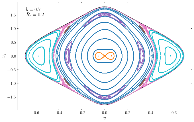
Comparing this surface of section to that at \(E=-0.87\) from Section 14.2 shows that this surface of section looks quite different. The \(E=-0.87\) surface of section was dominated by box orbits, with only a small fraction of loop orbits. At \(E=0\), however, loop orbits make up a substantial fraction of the section at large distances from the center (the cyan curves above). Box orbits dominate the central part of the section (the dark blue curves above), but very close to the center a new family of orbits appears that avoids the center (the orange curves). Two more small families of regular orbits appear as well (the purple and brown curves), and there is a closed orbit inside of the box orbit region (the blue dots) and a chaotic orbit between the loop and box orbits (the pink dots0. All of the closed regular orbits shown here aside from that in the box-orbit region are stable: they are surrounded by qualitatively similar, non-closed orbits.

To further understand the new orbit families, let’s look at the four new types of closed orbits that we find in this surface of section:

figsize(12,4)
ts= numpy.linspace(0.,100.,100001)
for ii,orb in enumerate(['banana','pretzel','box','harbinger']):
    o= orbit_yvyE(closed[orb][0],closed[orb][1],E,pot=lp)
    o.integrate(ts,lp,method='dop853_c')
    subplot(1,4,ii+1)
    o.plot(gcf=True,
           xrange=[-1.,1.] if ii == 0 else [-0.675,0.675],
           yrange=[-0.75,0.75])
    plot([0.],[0.],'ko',ms=7.)
    if ii > 0:
        gca().get_yaxis().get_label().set_visible(False)
        yticks([])
tight_layout();

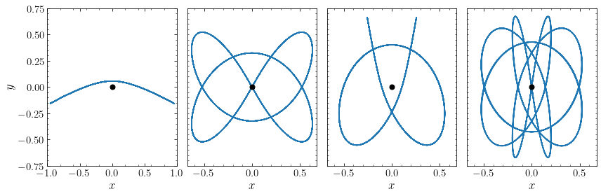
The orbit on the left corresponds to the orange dot in the surface of section and it is what the closed long-axis box orbit becomes at this energy. That is, the straight \(y=0\) orbit at \(E=-0.87\) becomes a bent orbit at \(E=0\). Because of its shape, this type of orbit is known as a banana orbit. The closed banana orbit avoids the center and is therefore centrophobic. The other closed orbits are more complicated. We see that two of them are centrophilic and pass through the origin, while the orbit that is surrounded by box orbits (the third orbit here, which corresponds to the blue points in the surface of section) is centrophobic. We will refer to all orbits like this as boxlets. Some examples of boxlets in the \(1/r\) cusps of dark-matter halos are shown in Section 14.4.3 below.

To get a better sense of how these orbits develop, let’s look at animations for some of these closed orbits. Animating the banana orbit with o.animate(d1='x',d2='y'), we get

Play

Pause

Speed x 2

Speed / 2

Replay

Similarly, for the pretzel-like orbit, we get

Play

Pause

Speed x 2

Speed / 2

Replay

We can now increase the central density by reducing the size of the core. First we will keep the core radius at a finite value, such that there is still a small harmonic core to the potential at \(R \ll R_c\), but from the vantage of the \(E=0\) orbits that we are considering, this region is almost negligible. For \(R_c = 0.05\), the surface of section looks as follows:

from galpy.potential import LogarithmicHaloPotential, evaluatePotentials
from galpy.orbit import Orbit
from scipy import optimize
figsize(11,7)
def surface_section(xs,ys,vys):
    # Find points where the orbit crosses x from - to +
    shiftxs= numpy.roll(xs,-1)
    indx= (xs[:-1] < 0.)*(shiftxs[:-1] > 0.)
    return (ys[:-1][indx],vys[:-1][indx])
def orbit_yvyE(y,vy,E,pot=None):
    """Returns Orbit at (x=0,y,vy) with given E"""
    return Orbit([y,vy,numpy.sqrt(2.*(E-evaluatePotentials(pot,y,0.,phi=numpy.pi/2.)
                                  -vy**2./2)),numpy.pi/2.])
def zvc(y,E,pot=None):
    """Returns the maximum v_y at this y and this
       energy: the zero-velocity curve"""
    return numpy.sqrt(2.*(E-evaluatePotentials(pot,y,0.,phi=numpy.pi/2.)))
lp= LogarithmicHaloPotential(amp=1.,b=0.7,core=0.05)
E= 0.
ts= numpy.linspace(0.,10000.,10000001)
# Location of closed orbits in [y,vy]
closed= {'banana': [0.1252,0.],
         'box': [], # not closed!
         'fish': [0.1741,1.099995],
         'pretzel': [0.001,1.795],
         'loop': [0.56,0.]}
nonclosed= {'banana': [[0.02,0.],[0.05,0.]],
            'box': [[0.3,0.],[0.25,0.],[0.33,0.],[0.06,1.25],[0.35,0.],[0.39,0.]],
            'fish': [[0.18,1.],[0.09,1.5]],
            'pretzel': [[0.04,1.55]],
            'loop': [[0.48,0.],[0.44,0.],[0.52,0.],[0.39,0.],[0.37,0.]]}
colors= {'banana': 'tab:orange',
         'fish': 'tab:green',
         'pretzel': 'tab:purple',
         'box': 'tab:blue',
         'loop': 'tab:cyan'}
for orb in closed:
    for sgn in [-1,1]:
        if not orb == 'box':
            o= orbit_yvyE(sgn*closed[orb][0],closed[orb][1],E,pot=lp)
            o.integrate(ts,lp,method='dop853_c')
            sectys,sectvys=surface_section(o.x(ts),o.y(ts),o.vy(ts))
            marker= '.'
            plot(sectys,sectvys,marker,mec='none',zorder=2,
                 mfc=colors[orb])
        for nonc in nonclosed[orb]:
            o= orbit_yvyE(sgn*nonc[0],nonc[1],E,pot=lp)
            o.integrate(ts,lp,method='dop853_c')
            sectys,sectvys=surface_section(o.x(ts),o.y(ts),o.vy(ts))
            marker= '.'
            plot(sectys,sectvys,marker,ms=3.,mec='none',zorder=2,mfc=colors[orb])
# Also plot the zero-velocity curve, first find min x at which it exists
miny= optimize.brentq(lambda y: E-evaluatePotentials(lp,y,0.,phi=numpy.pi/2.),
                      0.01,0.9)-1e-10
ys= numpy.linspace(-miny,miny,201)
plot(ys,zvc(ys,E,pot=lp),color='k',zorder=0)
plot(ys,-zvc(ys,E,pot=lp),color='k',zorder=1)
galpy_plot.text(r'$b=0.7$'+'\n'+r'$R_c=0.05$',top_left=True,size=18.)
xlabel(r'$y$')
ylabel(r'$v_y$');

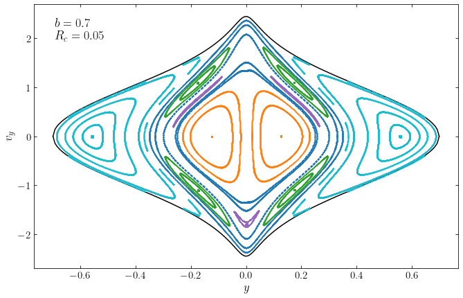
The surface of section has now dramatically changed. Loop orbits and banana orbits take up a very large fraction of the section, with box orbits relegated to the small area between the loop and banana orbits. But in this area, two new minor orbit families appear that take up a significant fraction and squeeze the box orbits further. There are thus very few box orbits at this energy in this potential and the few that exist are quite extended in \(y\) and therefore not very suitable for sustaining the non-axisymmetric structure of the potential. To further understand the new minor orbit families, we look at the closed orbits in the surface of section that are the parents of non-loop orbits:

figsize(10,4)
ts= numpy.linspace(0.,100.,100001)
labels= [r'$\mathrm{banana}$',
         r'$\mathrm{fish}$',
         r'$\mathrm{pretzel}$']
for ii,orb in enumerate(['banana','fish','pretzel']):
    o= orbit_yvyE(closed[orb][0],closed[orb][1],E,pot=lp)
    o.integrate(ts,lp,method='dop853_c')
    subplot(1,3,ii+1)
    o.plot(gcf=True,
           xrange=[-1.,1.],
           yrange=[-0.75,0.75])
    plot([0.],[0.],'ko',ms=7.)
    if ii > 0:
        gca().get_yaxis().get_label().set_visible(False)
        yticks([])
    galpy_plot.text(labels[ii],top_left=True,size=24.)
tight_layout();

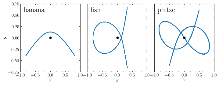
We see that we again have a banana orbit that parents the large family of banana orbits near the center of the surface of section (the orange curves). The parent of the green curves in the surface of section is the second closed orbit, which looks like a fish and is therefore known as a fish orbit. The third closed orbit, the parent of the purple curves, twists around a few times and we’ll refer to it as a pretzel orbit. The remarkable property of these orbits is that they all avoid the center and are thus centrophobic; there are no closed orbits that pass through the center.

Finally, we can set the core radius to zero and look at orbits in the cuspy logarithmic potential. The surface of section now looks as follows (see Miralda-Escude & Schwarzschild 1989):

from galpy.potential import LogarithmicHaloPotential, evaluatePotentials
from galpy.orbit import Orbit
from scipy import optimize
figsize(11,7)
def surface_section(xs,ys,vys):
    # Find points where the orbit crosses x from - to +
    shiftxs= numpy.roll(xs,-1)
    indx= (xs[:-1] < 0.)*(shiftxs[:-1] > 0.)
    return (ys[:-1][indx],vys[:-1][indx])
def orbit_yvyE(y,vy,E,pot=None):
    """Returns Orbit at (x=0,y,vy) with given E"""
    return Orbit([y,vy,numpy.sqrt(2.*(E-evaluatePotentials(pot,y,0.,phi=numpy.pi/2.)
                                  -vy**2./2)),numpy.pi/2.])
def zvc(y,E,pot=None):
    """Returns the maximum v_y at this y and this
       energy: the zero-velocity curve"""
    return numpy.sqrt(2.*(E-evaluatePotentials(pot,y,0.,phi=numpy.pi/2.)))
lp= LogarithmicHaloPotential(amp=1.,b=0.7,core=0.)
E= 0.
ts= numpy.linspace(0.,10000.,10000001)
# Location of closed orbits in [y,vy]
closed= {'banana': [0.12775,0.],
         'fish': [0.16,1.15],
         'pretzel': [0.34775,0.],
         '53': [0.2905,0.],
         'loop': [0.5575,0.]}
nonclosed= {'banana': [[0.03,0.],[0.07,0.],[0.0125,0.]],
            'fish': [[0.05,2.],[0.12,1.2]],
            'pretzel': [[0.343,0.],[0.105,1.8]],
            '53': [[0.31,0.],],
            'loop': [[0.5,0.],[0.4,0.],[0.36,0.]]}
colors= {'banana': 'tab:orange',
         'fish': 'tab:green',
         'pretzel': 'tab:purple',
         '53': 'tab:blue',
        'loop': 'tab:cyan'}
for orb in closed:
    for sgn in [-1,1]:
        o= orbit_yvyE(sgn*closed[orb][0],closed[orb][1],E,pot=lp)
        o.integrate(ts,lp,method='dop853_c')
        sectys,sectvys=surface_section(o.x(ts),o.y(ts),o.vy(ts))
        marker= '.'
        plot(sectys,sectvys,marker,mec='none',zorder=2,
             mfc=colors[orb])
        for nonc in nonclosed[orb]:
            o= orbit_yvyE(sgn*nonc[0],nonc[1],E,pot=lp)
            o.integrate(ts,lp,method='dop853_c')
            sectys,sectvys=surface_section(o.x(ts),o.y(ts),o.vy(ts))
            marker= '.'
            plot(sectys,sectvys,marker,ms=3.,mec='none',zorder=2,mfc=colors[orb])
# Also plot the zero-velocity curve, first find min x at which it exists
miny= optimize.brentq(lambda y: E-evaluatePotentials(lp,y,0.,phi=numpy.pi/2.),
                     0.01,0.9)-1e-10
ys= numpy.linspace(-miny,miny,201)
plot(ys,zvc(ys,E,pot=lp),color='k',zorder=0)
plot(ys,-zvc(ys,E,pot=lp),color='k',zorder=1)
galpy_plot.text(r'$b=0.7$'+'\n'+r'$R_c=0.0$',top_left=True,size=18.)
xlabel(r'$y$')
ylabel(r'$v_y$');

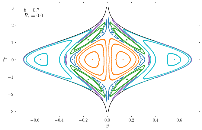
We see that box orbits have now completely disappeared and are instead replaced by different families of boxlets. All of these are regular orbits, although there is some mild chaos in this surface of section that is not shown here and has only a minor effect on the orbital structure. The closed orbits at the center of the boxlet orbit families are the following:

figsize(14,4)
ts= numpy.linspace(0.,100.,100001)
labels= [r'$\mathrm{banana}$',
         r'$\mathrm{fish}$',
         r'$\mathrm{pretzel}$',
         r'$\mathrm{5:3\ pretzel}$']
for ii,orb in enumerate(['banana','fish','pretzel','53']):
    o= orbit_yvyE(closed[orb][0],closed[orb][1],E,pot=lp)
    o.integrate(ts,lp,method='dop853_c')
    subplot(1,4,ii+1)
    o.plot(gcf=True,
           xrange=[-1.,1.],
           yrange=[-0.85,0.85])
    plot([0.],[0.],'ko',ms=7.)
    if ii > 0:
        gca().get_yaxis().get_label().set_visible(False)
        yticks([])
    galpy_plot.text(labels[ii],top_left=True,size=24.)
tight_layout();

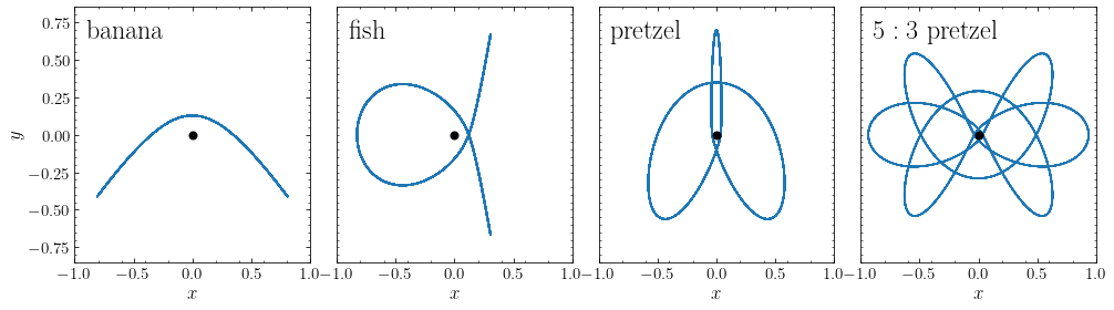
We see again the banana and the fish and two types of pretzel orbits (the second one a rather complicated pretzel). All of these closed orbits are again centrophobic. They give rise to non-closed orbit families with qualitatively similar behavior to the closed orbits:

figsize(14,4)
ts= numpy.linspace(0.,100.,100001)
labels= [r'$\mathrm{banana}$',
         r'$\mathrm{fish}$',
         r'$\mathrm{pretzel}$',
         r'$\mathrm{5:3\ pretzel}$']
for ii,orb in enumerate(['banana','fish','pretzel','53']):
    o= orbit_yvyE(nonclosed[orb][0][0],nonclosed[orb][0][1],E,pot=lp)
    o.integrate(ts,lp,method='dop853_c')
    subplot(1,4,ii+1)
    o.plot(gcf=True,
           xrange=[-1.,1.],
           yrange=[-0.85,0.85])
    plot([0.],[0.],'ko',ms=7.)
    if ii > 0:
        gca().get_yaxis().get_label().set_visible(False)
        yticks([])
    galpy_plot.text(labels[ii],top_left=True,size=24.)
tight_layout();

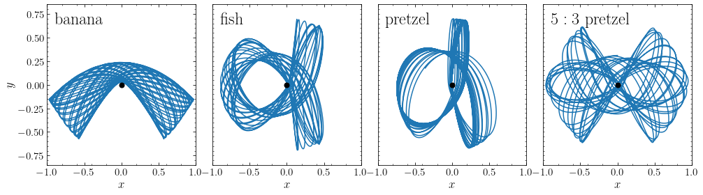
It’s clear that all of these orbits are quite thick in the \(y\) direction and are therefore not very suitable for supporting the non-axisymmetric structure of the potential. Thus, we see that as the cored logarithmic potential becomes the singular, cuspy logarithmic potential, all box orbits cease to exist and that they are replaced by centrophobic, thick boxlets.

14.4.3. The shape evolution of dark matter halos

\label{sec-triaxialorbs-dmhalos-shape}

As discussed in the previous section, the \(1/r\) inner-density cusps of dark-matter halos are weak enough that supporting long-term-stable triaxial configurations is relatively straightforward. Thus, it is not surprising that dark-matter halos formed in simulations that only include dark matter and its collisionless evolution are able to remain triaxial for the age of the Universe (e.g., Frenk et al. 1988; Dubinski & Carlberg 1991; Jing & Suto 2002). Simulations that include the dissipationless physics of the gaseous component, as well as star formation and its associated feedback processes, form a central galaxy at the bottom of the dark-matter potential well. In such more realistic simulations, dark matter halos are generally rounder, that is, much closer to axisymmetric and gently oblate rather than strongly prolate (e.g., Dubinski 1994; Gustafsson et al. 2006; Abadi et al. 2010; Kazantzidis et al. 2010; Chua et al. 2019). Detailed analyses of the changes to halo orbits induced by the growth of the central galaxy demonstrate that the reason for these shape changes are undramatic changes to the shapes of the orbit, at least for realistic gaseous and stellar density profiles (e.g., Debattista et al. 2008; Valluri et al. 2010). Only if a very compact central galaxy is formed does strong scattering significantly change the nature of the dark matter orbits in an irreversible manner (that is, chaotically).

Box orbits form the backbone of stable triaxial mass configurations and what happens to the box orbits when a central galaxy forms therefore determines how the triaxial figure evolves. To investigate this, we can see what happens when we grow a stellar disk inside of a triaxial dark-matter halo with typical values of the axis ratios \(b/a = 0.7\) and \(c/a = 0.5\) (\(T=0.68\); see Chapter 13.1). We use values such that the dark matter halo and the disk are similar to the Milky Way’s, in units where the Sun is at \(R=1\) from the center; we use a Hernquist profile rather than a NFW profile such that the model has finite mass, but this does not affect the central structure. Let’s see what happens to a typical narrow box orbit at \(z=0\) that extends out to the radius of the Sun:

from galpy.potential import (TriaxialHernquistPotential,
                             MiyamotoNagaiPotential,
                             DehnenSmoothWrapperPotential)
from galpy.orbit import Orbit
hp= TriaxialHernquistPotential(amp=28.,a=2.,b=0.7,c=0.5)
mp= MiyamotoNagaiPotential(amp=0.6,a=1./3.,b=1./30.) # approx 1./10 mass within r=20.
o= Orbit([1.,0.78,0.1,0.])
ts= numpy.linspace(0.,100.,1001)
o.integrate(ts,hp)
figsize(10,4)
o.plot(label=r'$\mathrm{Before}$');
growts= numpy.linspace(0.,300.,1001) # approx. adiabatic growth
o.integrate(growts,hp+DehnenSmoothWrapperPotential(pot=mp,tform=0.,tsteady=growts[-1]))
o= o(growts[-1])
o.integrate(ts,hp+mp)
o.plot(label=r'$\mathrm{After\ adiabatic\ disk\ growth}$',overplot=True)
ylim(-0.6,0.6)
gca().set_aspect('equal')
legend(frameon=False,fontsize=18);

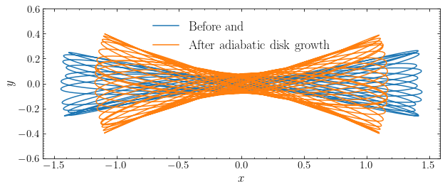
We show the orbit before and after the adiabatic growth of the disk—adiabatic meaning that we grow the disk on a timescale that is much larger than the typical orbital timescales. There are two noticeable change to the orbit. The first is that the orbit after the disk is grown does not extend to as large radii as before the disk growth. This is called adiabatic contraction (Blumenthal et al. 1986) and it occurs whenever a centrally-concentrated distribution of mass grows within a dark-matter halo (whether it is a disk, bulge, or elliptical galaxy). Adiabatic causes the density of the dark matter to increase in the inner part of the halo, but it does not directly affect the shape, unless it also steepens the inner density cusp significantly away from \(1/r\), such that box orbits would be significantly deformed or destroyed. However, realistic central galaxies have a shallow enough density profile themselves that they do not significantly change the cusp, which remains \(\approx 1/r\) (Gnedin et al. 2004).

The second noticeable change between the box orbit before and after the adiabatic disk growth is that it fans out more after disk growth. All of the mass associated with this orbit would therefore be more spread out along the direction \(y\) along which the potential is flattened. This happens to all box orbits and the overall effect of the growth of the disk is therefore to make the triaxiality-supporting box orbits, and therefore the entire mass distribution, rounder. To see this more clearly, we can look at an illustrative surface of section. Considering orbits within the \(z=0\) plane with the same energy as the orbit above, the surface of section \((y,v_y)\) looks as follows:

from galpy.potential import TriaxialHernquistPotential
from galpy.orbit import Orbit
from scipy import optimize
figsize(11,7)
def surface_section(xs,ys,vys):
    # Find points where the orbit crosses x from - to +
    shiftxs= numpy.roll(xs,-1)
    indx= (xs[:-1] < 0.)*(shiftxs[:-1] > 0.)
    return (ys[:-1][indx],vys[:-1][indx])
def orbit_yvyE(y,vy,E,pot=None):
    """Returns Orbit at (x=0,y,vy) with given E"""
    return Orbit([y,vy,numpy.sqrt(2.*(E-evaluatePotentials(pot,y,0.,phi=numpy.pi/2.)
                                  -vy**2./2)),numpy.pi/2.])
def zvc(y,E,pot=None):
    """Returns the maximum v_y at this y and this
       energy: the zero-velocity curve"""
    return numpy.sqrt(2.*(E-evaluatePotentials(pot,y,0.,phi=numpy.pi/2.)))
hp= TriaxialHernquistPotential(amp=28.,a=2.,b=0.7,c=0.5)
E= -1.8
ts= numpy.linspace(0.,1000.,1000001)# Book fig. produced with ts= numpy.linspace(0.,10000.,10000001)
# Location of closed orbits in [y,vy]
closed= {'banana': [0.00655,0.],
         'fish': [0.1127,0.49],
         'pretzel': [0.33338,0.],
         'pretzel2': [0.44355,0.],
         'box': None,
         'loop': [0.905,0.]}
nonclosed= {'banana': [[0.01,0.]],
            'fish': [[0.14,0.5],[0.12,0.2]],
            'pretzel': [[0.345,0.],[0.365,0.]],
            'box': [[0.03,0.],[0.07,0.],[0.1,0.],[0.15,0.],[0.2,0.],
                    [0.25,0.],[0.275,0.],[0.29,0.],[0.4,0.],[0.42,0.]],
            'pretzel2': [[0.44,0.]],
            'loop': [[0.7,0.],[0.6,0.],[0.5,0.],[0.47,0.],[0.46,0.]]}
colors= {'banana': 'tab:orange',
         'fish': 'tab:green',
         'pretzel': 'tab:purple',
         'pretzel2': 'tab:brown',
         'box': 'tab:blue',
         'loop': 'tab:cyan'}
for orb in closed:
    for sgn in [-1,1]:
        if not closed[orb] is None:
            o= orbit_yvyE(sgn*closed[orb][0],closed[orb][1],E,pot=hp)
            o.integrate(ts,hp,method='dop853_c')
            sectys,sectvys=surface_section(o.x(ts),o.y(ts),o.vy(ts))
            marker= '.'
            plot(sectys,sectvys,marker,mec='none',zorder=2,
                 mfc=colors[orb])
        for nonc in nonclosed[orb]:
            o= orbit_yvyE(sgn*nonc[0],nonc[1],E,pot=hp)
            o.integrate(ts,hp,method='dop853_c')
            sectys,sectvys=surface_section(o.x(ts),o.y(ts),o.vy(ts))
            marker= '.'
            plot(sectys,sectvys,marker,ms=3.,mec='none',zorder=2,mfc=colors[orb])
# Also plot the zero-velocity curve, first find min x at which it exists
miny= optimize.brentq(lambda y: E-evaluatePotentials(hp,y,0.,phi=numpy.pi/2.),
                     0.1,1.9)-1e-10
ys= numpy.linspace(-miny,miny,201)
plot(ys,[zvc(y,E,pot=hp) for y in ys],color='k',zorder=0)
plot(ys,[-zvc(y,E,pot=hp) for y in ys],color='k',zorder=1)
xlim(-1.35,1.35)
ylim(-2.3,2.3)
xlabel(r'$y$')
ylabel(r'$v_y$');

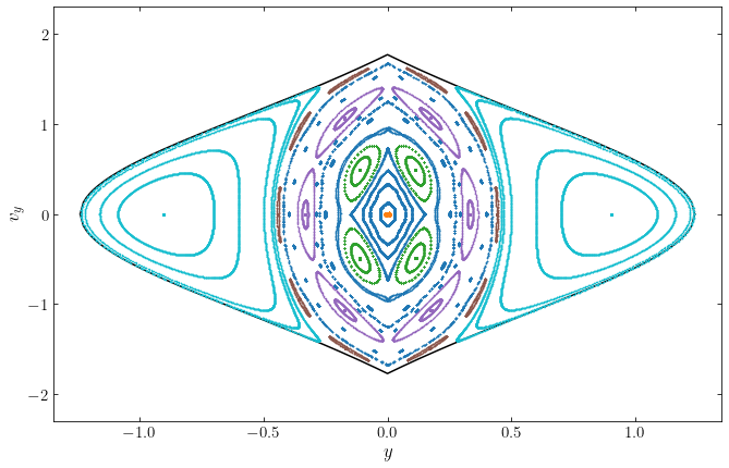
This surface of section has a similar structure to the cored and singular logarithmic potentials that we considered in the previous section. There is a small family of banana orbits at the very center and other minor orbit families consisting of ‘fish’- and ‘pretzel’-like boxlets, but a substantial fraction of the surface of section is occupied by the regular box orbits (the blue curves above) that provide the main support for triaxiality (there are also many loop orbits). The closed orbits in the minor orbit families look similar to those in the logarithmic potential above, but comparing them to those in the singular logarithmic potential above, we see that they are substantially flatter in \(y\) and therefore better able to provide support for the non-axisymmetric figure:

figsize(14,4)
ts= numpy.linspace(0.,100.,100001)
for ii,orb in enumerate(['banana','fish','pretzel','pretzel2']):
    o= orbit_yvyE(closed[orb][0],closed[orb][1],E,pot=hp)
    o.integrate(ts,hp,method='dop853_c')
    subplot(1,4,ii+1)
    o.plot(gcf=True,
           xrange=[-1.8,1.8],
           yrange=[-1.3,1.3])
    plot([0.],[0.],'ko',ms=7.)
    if ii > 0:
        gca().get_yaxis().get_label().set_visible(False)
        yticks([])
tight_layout();

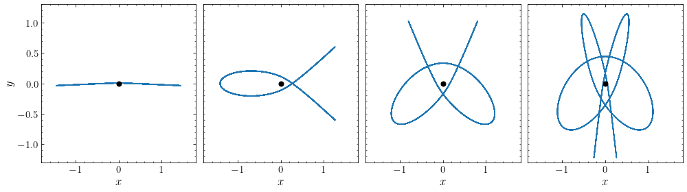
To see what these orbits evolve to, we create a similar surface of section of the orbits after we have grown the disk. Note that the result is not a constant-energy surface of section any longer, because the energy is not conserved during the adiabatic growth. But it is useful to look at this to see what a population of orbits at a given energy evolves into. The surface of section looks as follows:

from galpy.potential import TriaxialHernquistPotential
from galpy.orbit import Orbit
from scipy import optimize
figsize(11,7)
def surface_section(xs,ys,vys):
    # Find points where the orbit crosses x from - to +
    shiftxs= numpy.roll(xs,-1)
    indx= (xs[:-1] < 0.)*(shiftxs[:-1] > 0.)
    return (ys[:-1][indx],vys[:-1][indx])
def orbit_yvyE(y,vy,E,pot=None):
    """Returns Orbit at (x=0,y,vy) with given E"""
    return Orbit([y,vy,numpy.sqrt(2.*(E-evaluatePotentials(pot,y,0.,phi=numpy.pi/2.)
                                  -vy**2./2)),numpy.pi/2.])
def zvc(y,E,pot=None):
    """Returns the maximum v_y at this y and this
       energy: the zero-velocity curve"""
    return numpy.sqrt(2.*(E-evaluatePotentials(pot,y,0.,phi=numpy.pi/2.)))
hp= TriaxialHernquistPotential(amp=28.,a=2.,b=0.7,c=0.5)
mp= MiyamotoNagaiPotential(amp=0.6,a=1./3.,b=1./30.) # approx 1./10 mass within r=20.
E= -1.8
ts= numpy.linspace(0.,1000.,1000001)# Book fig. produced with ts= numpy.linspace(0.,10000.,10000001)
growts= numpy.linspace(0.,300.,1001)
# Location of closed orbits in [y,vy]
closed= {'banana': [0.00655,0.],
         'fish': [0.1127,0.49],
         'pretzel': [0.33338,0.],
         'pretzel2': [0.44355,0.],
         'box': None,
         'loop': [0.905,0.]}
nonclosed= {'banana': [[0.01,0.]],
            'fish': [[0.14,0.5],[0.12,0.2]],
            'pretzel': [[0.345,0.],[0.365,0.]],
            'box': [[0.03,0.],[0.07,0.],[0.1,0.],[0.15,0.],[0.2,0.],
                    [0.25,0.],[0.275,0.],[0.29,0.],[0.4,0.],[0.42,0.]],
            'pretzel2': [[0.44,0.]],
            'loop': [[0.7,0.],[0.6,0.],[0.5,0.],[0.47,0.],[0.46,0.]]}
colors= {'banana': 'tab:orange',
         'fish': 'tab:green',
         'pretzel': 'tab:purple',
         'pretzel2': 'tab:brown',
         'box': 'tab:blue',
         'loop': 'tab:cyan'}
for orb in closed:
    for sgn in [-1,1]:
        if not closed[orb] is None:
            o= orbit_yvyE(sgn*closed[orb][0],closed[orb][1],E,pot=hp)
            o.integrate(growts,hp+DehnenSmoothWrapperPotential(pot=mp,tform=0.,tsteady=growts[-1]),
                       method='dop853_c')
            o= o(growts[-1])
            o.integrate(ts,hp+mp,method='dop853_c')
            sectys,sectvys=surface_section(o.x(ts),o.y(ts),o.vy(ts))
            marker= '.'
            plot(sectys,sectvys,marker,ms=3.,mec='none',zorder=2,
                 mfc=colors[orb])
        for nonc in nonclosed[orb]:
            o= orbit_yvyE(sgn*nonc[0],nonc[1],E,pot=hp)
            o.integrate(growts,hp+DehnenSmoothWrapperPotential(pot=mp,tform=0.,tsteady=growts[-1]),
                       method='dop853_c')
            o= o(growts[-1])
            o.integrate(ts,hp+mp,method='dop853_c')
            sectys,sectvys=surface_section(o.x(ts),o.y(ts),o.vy(ts))
            marker= '.'
            plot(sectys,sectvys,marker,ms=3.,mec='none',zorder=2,mfc=colors[orb])
xlim(-1.35,1.35)
ylim(-2.3,2.3)
xlabel(r'$y$')
ylabel(r'$v_y$');

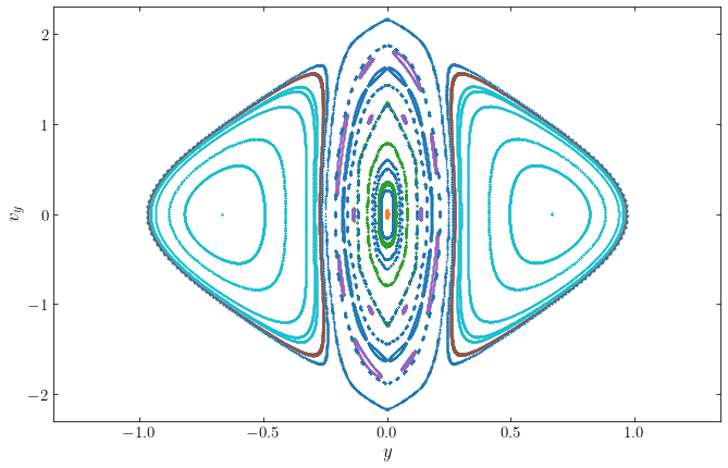
we have plotted the surface of section for the same axis limits to make it easily comparable to the original one. This surface of section confirms that the orbits by and large contract radially and expand in the \(y\) direction along which the mass distribution is flattened. The overall effect is thus to significantly round out the mass distribution. Indeed, it is clear both from the single orbit that we looked at above and the entire surface of section that the box orbits expand by a factor of \(\approx 1.5\) to \(2\) in the \(y\) direction. This is plenty to turn the \(b/a = 0.7\) flattening into a \(b/a \approx 1\) axisymmetric distribution. A similar effect in the \(z\) direction turns the \(c/a = 0.5\) into \(c/a \approx 0.75\) and the resulting shape is therefore an mildly oblate, axisymmetric dark matter halo, as seen in full \(N\)-body simulations.

In this surface of section, we have kept the color-coding of the different orbit families from the original surface of section. This makes it clear that some orbits change family due to the adiabatic growth of the disk. A few examples of this are shown in the next figure:

def plot_orbit_change(y,vy):
    o= orbit_yvyE(y,vy,E,pot=hp)
    o.integrate(ts,hp,method='dop853_c')
    o.plot(gcf=True,xrange=[-1.49,1.49],yrange=[-1.49,1.49]);
    o= orbit_yvyE(y,vy,E,pot=hp)
    o.integrate(growts,hp+DehnenSmoothWrapperPotential(pot=mp,tform=0.,tsteady=growts[-1]),
               method='dop853_c')
    o= o(growts[-1])
    o.integrate(ts,hp+mp,method='dop853_c')
    o.plot(overplot=True)
    gca().set_aspect('equal')
figsize(14,4)
subplot(1,4,1)
plot_orbit_change(nonclosed['banana'][0][0],nonclosed['banana'][0][1])
subplot(1,4,2)
plot_orbit_change(nonclosed['fish'][-1][0],nonclosed['fish'][-1][1])
gca().get_yaxis().get_label().set_visible(False)
yticks([])
subplot(1,4,3)
plot_orbit_change(nonclosed['box'][-1][0],nonclosed['box'][-1][1])
gca().get_yaxis().get_label().set_visible(False)
yticks([])
subplot(1,4,4)
plot_orbit_change(nonclosed['pretzel2'][-1][0],nonclosed['pretzel2'][-1][1])
gca().get_yaxis().get_label().set_visible(False)
yticks([])
tight_layout();

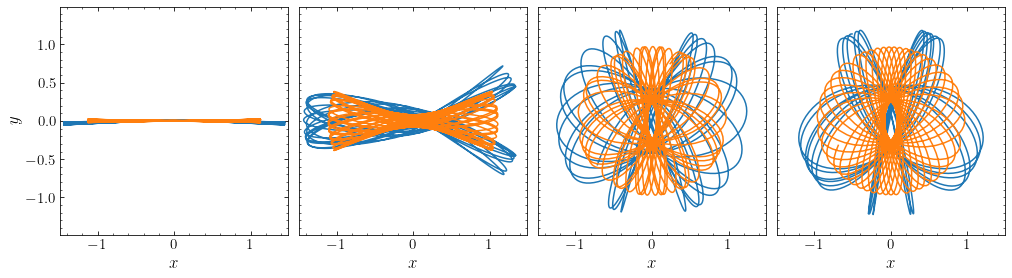
This figure demonstrates a few important aspects of the family changes. Boxlet families are largely turned into regular box orbits: we see how a banana orbit and a fish orbit turn into regular box orbits. However, this does not significantly change the overall shape of the spatial extent of the original orbit. Similarly, we see how a box orbit and a pretzel orbit become loop orbits after the growth of the disk. But again, while the orbits contract, the overall shape of their spatial extent is similar. Therefore, the effect of orbit-family changes on the shape of the dark matter halo is limited. Shape changes due to the growth of baryonic disks are therefore largely caused by the fact that they make narrow box orbits rounder rather than by significant changes to the types of orbits that are populated.

The discussion here has focused on the effect of the adiabatic growth of a central galactic disk. But in addition to deepening the gravitational potential well, gas cooling and star formation is also accompanied by energetic feedback processes from stellar winds and supernova explosions for galaxies like the Milky Way and smaller and by feedback from accretion of gas onto the central supermassive black hole in larger galaxies. These processes can transfer energy and momentum to the dark matter halo and this happens in a largely non-adiabatic manner (that is, fast compared to the orbital time scale). This transfer of, e.g., energy will further effect the orbits of halo particles. The adiabatic contraction that we witnessed above will be particularly affected by these processes, because increasing the energy of the dark matter particles will tend to enlarge their orbits and reduce the central density (we discussed this in the context of dwarf galaxies in Chapter 7.7) . It is therefore likely that there are no lasting effects from adiabatic contraction in galaxies that we observe today. Feedback processes, however, do not strongly affect the shape further and certainly cannot reverse the trend towards more axisymmetric and more spherical shapes, because energy transfer from the baryons to the dark matter does not flatten or further populate the triaxiality-supporting box orbits. It is therefore a robust prediction that the shapes of the inner density profiles of dark matter halos with massive galaxies at their centers should be axisymmetric, oblate ellipsoids with a flattening that in detail depends on the relative mass and radial profile of the disk (e.g., Kazantzidis et al. 2010).