
5. Orbits in spherical mass distributions
“Orbits” are the trajectories that bodies travel on under the influence of gravity in a gravitational field. As discussed in the previous chapters, these trajectories can be computed using Newton’s second law
where \(\vec{g}(\vec{x})\) is the gravitational field, \(m\) is the mass of the body, and \(\ddot{\vec{x}}\) is the acceleration vector. As discussed in Section 3.1, because we can cancel the mass on both sides of this equation, the acceleration \(\ddot{\vec{x}}\) in a gravitational field is independent of the mass of the body. If, furthermore, the mass of the body is so small that it does not affect the evolution of the gravitational field, the entire orbit is independent of mass. This is typically the case for orbiting bodies in galaxies (stars, dark matter particles, but not for heavy bodies such as massive black holes and large satellite galaxies orbiting within a bigger galaxy) and such bodies are known as test particles. Because of this, we can typically ignore the actual mass \(m\) of bodies orbiting in a galactc gravitational field and consider familiar quantities such as the energy, momentum, angular momentum, and the Lagrangian or the Hamiltonian as that per unit mass. For example, the momentum per unit mass—or the specific momentum—is \(\dot{\vec{x}}\) and this is often referred to simply as the momentum.
Because the orbital trajectory is determined by the second-order differential equation \eqref{eq-newton-eom}, an orbit is fully determined by its initial phase-space coordinate \(\vec{w}_0 = (\vec{x}_0,\vec{v}_0)\) and phase-space is filled by a dense set of non-crossing orbits. Again, this is only the case when the mass is so small that it can be ignored, because otherwise the trajectory also depends on other properties of the body, such as its mass (for a massive black hole) or its mass profile (for a satellite galaxy). Thus, we can discuss the properties of orbits without specifying whether these are the orbits of low- or high-mass stars, neutron stars, black holes, dark-matter particles, or of any other body with mass \(\ll\) the mass of the gravitational system.
5.1. General properties of orbits in spherical potentials
Equation \(\eqref{eq-newton-eom}\), or equivalent forms of it derived in the Lagrangian or Hamiltonian formalism, is an ordinary differential equation that typically needs to be solved numerically. Only for a handful of galactic potentials can Equation \(\eqref{eq-newton-eom}\) be solved analytically. Even for most spherical potentials, the full solution of Equation \(\eqref{eq-newton-eom}\) needs to be numerical. We will discuss the numerical solution of Equation \eqref{eq-newton-eom} in detail in Chapter 19.2, but the important thing to note about this numerical solution is that it is not particularly difficult. Galactic gravitational fields and the orbits within them are typically very smooth and, as we discussed in Chapter 3.3, galactic bodies have typically performed only a few dozen orbits, and a few thousand at most. Thus, we can solve the equation of motion with simple methods, like a standard Runge-Kutta method that can be coded up in a few lines, and we do not need high precision, because numerical errors do not add up over long integration times.
Because we are dealing with spherical mass distributions, we will mostly work in spherical coordinates and will denote the three-dimensional position as \(\vec{r}\) rather than \(\vec{x}\) as a reminder of this. Because only the radial derivative of the potential is non-zero, the equation of motion in a spherical potential simplifies to
where \(\hat{\vec{r}}\) is the radial unit vector and \(\vec{r} = r\,\hat{\vec{r}}\) (with \(r = |\vec{r}|\) the magnitude of the radius). The force points along the radial direction.
Spherical symmetry implies invariance under any rotation around the center of the potential. By Noether’s theorem (Chapter 4.3), this implies the existence of a conserved quantity. This quantity is the (specific) angular momentum vector
the cross product of the position vector and the velocity vector. That the angular momentum vector is conserved is most easily demonstrated simply by taking its time derivative. In Chapter 4.1, we showed that the time derivative of the (specific) angular momentum is equal to the (specific) torque \(\vec{N}\) (with a slight abuse of notation, we use the same symbol for torque and specific torque)
the cross product in the third line is that of a vector with itself, which is zero. That the angular momentum vector is conserved implies that the orbit is constrained to the plane through the origin that is perpendicular to the angular momentum vector. We therefore only have to consider the motion in this plane. The magnitude of the angular momentum is \(L\). We use polar coordinates \((r,\psi)\) in this plane to most easily describe the dynamics (using \(\psi\) rather than our regular \(\phi\) as the angle coordinate, as a reminder that this is not the angle \(\phi\) in a cylindrical coordinate frame, rather it is the angle in the orbital plane). We can derive the equations of motion in this coordinate system using the Lagrangian formalism (Chapter 4.3), where the Lagrangian is in this case given by
The equations of motion in this plane for \(\Phi(r,\psi) \equiv \Phi(r)\) are found using Lagrange’s equations (4.23) and are given by
The second of these equations again simply states the conservation of the angular momentum \(L = r^2\,\dot{\psi}\) and is known as Kepler’s second law in the context of the point-mass potential (but it holds more generally).
The specific energy \(E\) of an orbit in a spherical potential is given by
where we have replaced \(\dot{\psi}\) with \(L\) using Equation \(\eqref{eq-eom-spher-angle}\). As shown in Section 4.1, this specific energy is conserved if the potential \(\Phi(r)\) does not explicitly depend on time. Because the angular momentum is conserved, the equation of motion for \(r\) in Equation \(\eqref{eq-eom-spher-r}\) can be re-written in terms of an effective potential \(\Phi_\mathrm{eff}(r;L)\) given by
where we add \(L\) as an argument to the effective potential to make it explicitly clear that the effective potential is different for orbits with different specific angular momentum. The specific energy from Equation \(\eqref{eq-energy-spherpot}\) is then simply
The specific energy can therefore be thought of as a radial energy.
The energy and angular momentum work together to restrict the part of physical space that an orbit can occupy. Because for typical smooth galactic potentials \(\Phi(r)\) increases with increasing \(r\), energy conservation restricts orbits with energy \(E\) to those \(r\) with \(\Phi(r) \leq E\), which restricts bound orbits to \(r \leq r_{\mathrm{max}}(E)\) for which \(\Phi(r_\mathrm{max}) \leq E\), but allows orbits to reach \(r=0\); unbound orbits have \(E > \Phi_\infty\) and therefore have no \(r_{\mathrm{max}}(E)\) (potentials that do not converge at \(\infty\) therefore only have bound orbits).
The conservation of angular momentum in a spherical potential changes this restriction to \(\Phi_\mathrm{eff}(r;L) \leq E\). Like the potential itself, the effective potential decreases with decreasing \(r\) at large \(r\), but increases with decreasing \(r\) at small \(r\), because of the \(L^2/[2r^2]\) term, called the angular momentum barrier. Any spherical potential corresponding to a spherical density at most decreases as fast as the Kepler potential, \(\Phi(r) \propto 1/r\). Therefore, the increase in \(\Phi_\mathrm{eff}(r;L)\) at small \(r\) from the angular-momentum barrier \(L^2/[2r^2]\) always becomes larger than the decrease from \(\Phi(r)\) at small enough \(r\) and the \(L^2/[2r^2]\) term grows without bounds as \(r\rightarrow 0\). Therefore, for bound orbits with \(L \neq 0\), the equation \(\Phi_\mathrm{eff}(r;L) = E\) has two solutions, one at small \(r\) and one at large \(r\). Unbound orbits have no maximum \(r\), but as long as they have non-zero angular momentum, they do have a minimum \(r\).
Bound orbits therefore perform oscillations in \(r\) between a minimum and maximum value. Analogous to the perihelion and apohelion distances of orbits in the Keplerian potential for the solar system, these are known as the pericenter \(r_p\) and the apocenter \(r_a\), respectively. Because these radii are minima and maxima of \(r(t)\), we can find them by solving \(\dot{r} = 0\). Using Equation \(\eqref{eq-energy-spherpot}\), we can easily solve for these by solving \(\dot{r}^2 = 0\)
which is the same as solving \(\Phi_\mathrm{eff}(r;L) = E\), but makes it clear that these radii are turning points of the orbit. In general, this equation needs to be solved numerically. Circular orbits have a constant radius and therefore \(r_p = r_a\). A convenient quantity to quantify the circularity of an orbit is given by the orbital eccentricity \(e\), which can be defined as
For a circular orbit \(e=0\), while orbits that are close to unbound have \(r_a \gg r_p\) and therefore \(e \rightarrow 1\) as \(r_a\) grows.
The time necessary to travel from pericenter to apocenter and back is known as the radial period \(T_r\). This period can be computed as
where we used Equation \(\eqref{eq-spherpot-drdt}\). The radial period describes the motion in the radial direction only. The motion of a body in a spherical potential in the azimuthal \(\psi\) direction also has a period associated with it, the azimuthal period \(T_\psi\) (or the rotational period). This is most easily computed by first calculating the change \(\Delta \psi\) in \(\psi\) over a radial period and then computing the number of radial periods necessary to complete one full \(\psi\) rotation. We have that
where we used Equation \(\eqref{eq-spherpot-drdt}\) and Equation \(\eqref{eq-eom-spher-angle}\) to substitute \(\mathrm{d}r/\mathrm{d}t\) and \(\mathrm{d}\psi/\mathrm{d}t\), respectively. The azimuthal period is then
where we need the absolute value of \(\Delta \psi\), because \(\Delta \psi\) can be negative. All of the quantities \(T_r\), \(\Delta \psi\), and \(T_\psi\) typically need to be computed numerically. Some care is necessary in this numerical calculation, because the integrands integrably diverge at the end-points of the integration interval (see Press et al. 2007 for methods for dealing with this situation). The radial and azimuthal frequencies are simply equal to \(2\pi\) over the radial and azimuthal period.
5.2. Orbits in specific spherical potentials
To illustrate the concepts introduced in the previous subsection, we consider orbital properties in a few simple spherical potentials.
5.2.1. Orbits in the homogeneous sphere
The homogeneous sphere (see Section 3.4.2) has particularly simple orbits. First, we re-write the potential for the homogeneous sphere from Equation (3.41) inside of its limiting radius as
where we have dropped the constant term and we have written the amplitude in terms of \(\omega^2 = 4\pi\,G\,\rho_0/3\). We only consider orbits that remain at \(r < R\). The equations for the homogeneous sphere are in fact most easily solved in cartesian coordinates rather than in polar coordinates as in Equation \(\eqref{eq-eom-spher-r}\), so we write this potential in cartesian coordinates (assuming that the orbital plane is at \(z=0\)):
The equations of motion are therefore
These have the solution
This solution describes an ellipse, with the center at the origin of the mass distribution (\(r=0\)). Note that these are not Keplerian orbits, even though Keplerian orbits are also ellipses; as we will see below, Keplerian orbits are ellipses with the origin of the mass distribution at the focus of the ellipse, not at the center of the ellipse as for the homogeneous sphere. This solution has four constants that need to be determined from the initial condition of the orbit (remember that we are working in the orbital plane, which is constant, and there are therefore only two positions and velocities that count; the position and velocity perpendicular to this plane are zero at all times). These constants are (i+ii) the semi-major and semi-minor axes of the ellipse, \(a\) and \(b\) respectively, (iii) the orientation of the ellipse within the plane, and (iv) the position along the orbit at \(t=0\). Let’s fix the latter two of these by orienting the ellipse such that the semi-major axis is along \(x\) and the orbit is at \(y=0\) at positive \(x\) at \(t=0\):
It is then straightforward to demonstrate that the energy and angular momentum are
or in terms of the eccentricity \(\varepsilon\) of the ellipse: \(\varepsilon = \sqrt{1-b^2/a^2}\)
The peri- and apocenter radii are simply
which directly follows from the properties of ellipses. Using Equations \(\eqref{eq-homogeneous-E}\) and \(\eqref{eq-homogeneous-L}\) it is also easy to show that \(E = \omega^2 a^2 / 2 + L^2 / [2a^2] = \omega^2 b^2/2 + L^2 / [2b^2]\). Note that the general definition of the orbital eccentricity \(e\) in Equation \(\eqref{eq-ecc-spher}\) does not agree with the standard definition of the eccentricity of an ellipse \(\varepsilon\) for orbits in the homogeneous sphere: \(e \neq \varepsilon\). We will see below that for orbits in the point-mass potential the two definitions do agree.
Because an ellipse goes through its pericenter and apocenter twice for each full rotation around the center, the radial period is half of the azimuthal period
Because the radial period is an integer fraction of the azimuthal period, all of the orbits in the homogeneous sphere close and are periodic. From the solved orbit in Equations \(\eqref{eq-homogeneous-orbit-1}\) and \(\eqref{eq-homogeneous-orbit-2}\) it is clear that the azimuthal period is simply \(\omega\) and therefore
The period of every orbit in the homogeneous sphere is therefore the same, the period does not depend on either the energy or angular momentum of the orbit. As we will see below, this is not generally the case. From Equation \(\eqref{eq-tr-tpsi-dpsi}\), we find that \(\Delta \psi\)
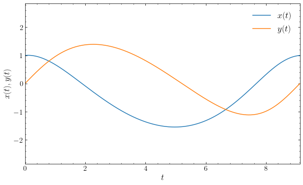
Let us look at an example of an orbit in the homogeneous sphere using galpy. We normalize the potential again such that \(v_c(r=1) = 1\) and use a size \(R\) such that the considered orbit never strays outside of the constant-density part of the potential. Using this normalization, \(\omega= 1\) and the period \(2\pi/\omega\) in \(x(t)\) and \(y(t)\) should be equal to \(2\pi\). Let’s integrate an orbit with initial condition
\((x,y,v_x,v_y) = (1.0,0.0,0.1,1.1)\) in the \(z=0\) plane (note that galpy requires initial conditions to be given in polar coordinates in this case and in general requires initial conditions in cylindrical coordinates). We plot the \(x(t)\) and \(y(t)\) behavior:
[4]:
from galpy import potential
from galpy.orbit import Orbit
figsize(10,6)
hp= potential.HomogeneousSpherePotential(normalize=1.,R=20.)
oh= Orbit([1.,0.1,1.1,0.])
ts= numpy.linspace(0.,2.*numpy.pi,1001)
oh.integrate(ts,hp)
oh.plotx(ylabel=r'$x(t),y(t)$',yrange=[-1.65,1.65],
        label=r'$x(t)$')
oh.ploty(label=r'$y(t)$',overplot=True)
legend(fontsize=18.,loc='upper right',frameon=False);
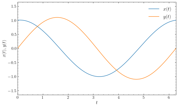
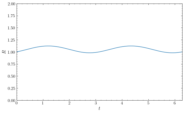
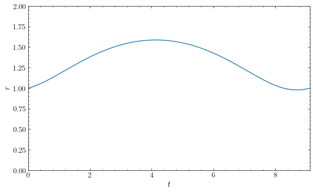
This demonstrates the sinusoidal behavior expected from Equations \(\eqref{eq-homogeneous-orbit-1}\) and \(\eqref{eq-homogeneous-orbit-2}\). The \(R(t)\) curve should have a period of half of that in \(x(t)\) and \(y(t)\); in this case it should be \(\pi\). This is indeed what we see when we look at the orbit in \(R(t)\):
[5]:
oh.plotR(yrange=[0.,2.]);
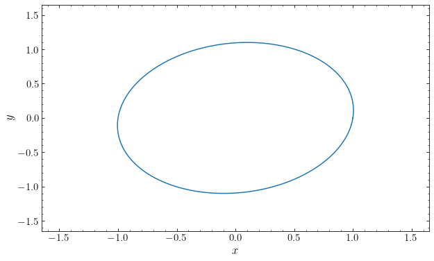
The orbit in the \((x,y)\) plane is indeed an ellipse with the center at the origin of the coordinate system:
[6]:
oh.plot(xrange=[-1.65,1.65],yrange=[-1.65,1.65]);
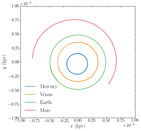
As another example, we consider what the orbits of the four inner solar-system planets would look like if the solar system were a homogeneous density rather than having almost all of the mass concentrated in the Sun (as we will consider in the next section). We setup a homogeneous sphere density in galpy with a density such that the mass within a sphere of 1 AU is one solar mass (thus, the orbit of the Earth should be similar as in the true potential):
[10]:
import astropy.units as u
# necessary to transfer the solar system's unit system to the potential
from galpy.util.conversion import get_physical
o= Orbit.from_name('solar system')[:4]
hp= potential.HomogeneousSpherePotential(\
        amp=2.*numpy.pi/3.*(u.Msun/(4.*numpy.pi*(u.AU)**3./3.)),R=10.*u.AU,
        **get_physical(o))
Then we integrate the orbits of the inner solar-system planets for just over one year and plot the resulting orbits (galpy always works in kpc, hence the funny numbers):
[7]:
ts= numpy.linspace(0.,1.1,251)*u.yr
o.integrate(ts,hp)
figsize(7,7)
o.plot(d1='x',d2='y',xrange=[-1e-8,1e-8],yrange=[-1e-8,1e-8],
       label=[r'$\mathrm{{{planet}}}$'.format(planet=planet)
              for planet in Orbit.from_name('solar system').name[:4]])
legend(fontsize=18.,loc='upper right',frameon=False);
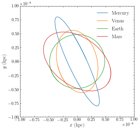
We see that the orbits are ellipses that all close after one year. The orbit of the Earth is almost circular, just like in the true point-mass potential, but the orbits of the other planets are much more eccentric than their true orbits. Mercury, the innermost planet, has the most eccentric orbit and the most different orbit from its true orbit. This is because the homogeneous density is the most different for Mercury for the way we have set it up.
The following animation (generated with o.animate(d1='x',d2='y')) shows the orbits of the innermost solar-system planets in the homogeneous density sphere. It clearly demonstrates that the period of all of the orbits is the same:
5.2.2. Orbits in the Kepler potential
Orbits in the homogeneous sphere are about as simple as orbits can get: bodies travel around ellipses at an angular rate that is independent of their energy and angular momentum (or equivalently, of their semi-major axis and eccentricity). Orbits in the Kepler potential are slightly more complicated.
To solve the equations of motion for orbits in the Kepler potential, we use Equation \(\eqref{eq-eom-spher-angle}\) to replace the time derivative with an azimuthal derivative
and then we re-write Equation \(\eqref{eq-eom-spher-r}\) in terms of \(u=1/r\). For general potentials this gives
and for the specific case of a Kepler potential, this simplifies to
This is the equation of a forced harmonic oscillator with constant forcing, with solution
In terms of \(r(\psi)\) this is
The combination \(\psi-\psi_0\) is known as the true anomaly. Because \(r\) only depends on \(\psi\) through the cosine, it is clear that orbit closes after one azimuthal period and that \(T_r = T_\psi\). In fact, this is the equation of an ellipse with the origin at one focus with semi-major axis \(a\) and eccentricity \(e\) given by
as long as \(e < 1\) (if \(e \geq 1\), the orbit is unbound and described by a parabola for \(e=1\) and a hyperbola for \(e > 1\)). That the orbits in the point-mas potential are closed ellipses is known as Kepler’s first law. In therms of the semi-major axis and eccentricity, Equation \eqref{eq-eom-kepler-orbit} becomes
The peri- and apocenter distances are then obtained by setting \(\psi = \psi_0\) and \(\psi = \pi+\psi_0\):
The orbital eccentricity \((r_a-r_p)/(r_a+r_p)\) is equal to \(e\) and the orbital eccentricity is therefore equal to the eccentricity of the Keplerian ellipse. This is the motivation for the general definition of the orbital eccentricity in Equation \(\eqref{eq-ecc-spher}\).
To compute the azimuthal period, rather than following the general expression of Equation \eqref{eq-tr-tpsi-dpsi}, we can use Equation \(\eqref{eq-eom-spher-angle}\) and \eqref{eq-eom-kepler-orbit-asellipse} to get
As argued above, the radial period \(T_r\) is equal to this azimuthal period. Using Equation \eqref{eq-kepler-semimajoraxis}, we can also write this as
which is Kepler’s third law.
To obtain the specific energy, we evaluate Equation \eqref{eq-spherpot-radialenergy} at the pericenter \(r = a(1-e)\), because there \(E = \Phi_\mathrm{eff}(r;L)\) and we can use Equation \eqref{eq-kepler-semimajoraxis} to simplify the resulting expression
In terms of the specific energy, the periods can also be expressed as
The radial period therefore only depends on the energy, it does not depend on the angular momentum.
An alternative parameterization of a Keplerian orbit uses a parameter called the eccentric anomaly \(\eta\) which is related to the true anomaly \(\psi-\psi_0\) through
In terms of the eccentric anomaly, we can write the orbit as
Perhaps somewhat surprisingly, the only time we will use this parameterization in this book is when discussing a simple model for the formation of dark-matter halos in Chapter 18.2.1!
Let’s look at the same orbit as we considered above in the homogeneous sphere potential, but now in a point-mass potential. We normalize the potential again such that \(v_c(r=1) = 1\) to get the same normalization as that we used above for the homogeneous sphere. We first compute \(a = (r_p+r_a)/2\) and get the radial period using Equation \(\eqref{eq-tr-tpsi-kepler}\):
[7]:
kp= potential.KeplerPotential(normalize=1.)
ok= Orbit([1.,0.1,1.1,0.])
rap= ok.rap(analytic=True,pot=kp)
rperi= ok.rperi(analytic=True,pot=kp)
a= 0.5*(rap+rperi)
Tr= 2.*numpy.pi*a**1.5
print("The radial period is %.2f" % Tr)
The radial period is 9.12
and then we integrate the orbit for \(t = T_r\):
[8]:
ts= numpy.linspace(0.,Tr,1001)
ok.integrate(ts,kp)
figsize(10,6)
ok.plotx(ylabel=r'$x(t),y(t)$',yrange=[-2.85,2.85],
        label=r'$x(t)$')
ok.ploty(label=r'$y(t)$',overplot=True)
legend(fontsize=18.,loc='upper right',frameon=False);
We see that the orbit is indeed periodic with a period equal to \(T_r\) also in \(r(t)\):
[9]:
ok.plotr(yrange=[0.,2.]);
The orbit covers a much larger range in \(r\) than the same initial conditions in the homogeneous sphere. Finally, let’s compare the orbits in the \((x,y)\) plane:
[14]:
ok.plot(xrange=[-2.2,2.2],yrange=[-2.2,2.2],
        label=r'$\mathrm{Point\ mass}$')
oh.plot(label=r'$\mathrm{Homogeneous\ sphere}$',overplot=True)
gca().set_aspect('equal')
legend(fontsize=18.,loc='upper right',frameon=False);
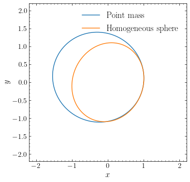
This clearly demonstrates that both orbits are ellipses, but that the origin is at the center of the ellipse for the homogeneous sphere, while it is at the focus of the ellipse for the point-mass potential.
As another example, we consider the orbits of planets in the solar system, now in the more realistic point-mass Kepler potential rather than the homogeneous density that we considered in the previous section. We set up a Kepler potential for the solar system as:
[13]:
o= Orbit.from_name('solar system')
kp= potential.KeplerPotential(amp=1.*u.Msun,**get_physical(o))
Then we integrate the orbits for just over one year and plot the resulting orbits of the inner-solar system planets:
[29]:
ts= numpy.linspace(0.,1.1,251)*u.yr
o.integrate(ts,kp)
figsize(7,7)
o[:4].plot(d1='x',d2='y',xrange=[-1e-8,1e-8],yrange=[-1e-8,1e-8],
           label=[r'$\mathrm{{{planet}}}$'.format(planet=planet)
              for planet in Orbit.from_name('solar system').name[:4]])
legend(fontsize=18.,loc='lower left',frameon=False);
We see that in the correct Kepler potential, the orbits of the planets are very close to circular and that, while the orbits of the planets inner to the Earth close after one year, the orbit of Mars does not. This is because the period increases with distance from the Sun according to Kepler’s third law (Equation \(\ref{eq-tr-tpsi-kepler}\)). Similarly, we can plot the orbits of the outer solar-system planets (we do not plot all eight on the same figure, because the range of scales is so large):
[30]:
o[4:].plot(d1='x',d2='y',xrange=[-3e-7,3e-7],yrange=[-3e-7,3e-7],
           label=[r'$\mathrm{{{planet}}}$'.format(planet=planet)
              for planet in Orbit.from_name('solar system').name[4:]])
legend(fontsize=18.,loc='lower left',frameon=False);
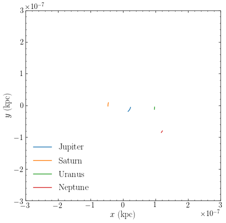
These are the orbits of the outer solar system planets over one year and we see that they do not move much along their orbits, again because their periods are much longer than one year due to Kepler’s third law. If we integrate for 160 years, the orbits of the three innermost outer-solar-system planets close
[39]:
ts= numpy.linspace(0.,160.,251)*u.yr
o.integrate(ts,kp)
o[4:].plot(d1='x',d2='y',xrange=[-3e-7,3e-7],yrange=[-3e-7,3e-7],
           label=[r'$\mathrm{{{planet}}}$'.format(planet=planet)
              for planet in Orbit.from_name('solar system').name[4:]])
legend(fontsize=18.,loc='lower left',frameon=False);
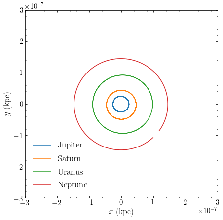
and the orbit of Neptune is just about to close (the period of Neptune is about 164 years).
An animation of the orbits of the outer solar-system planets using o[4:].animate(d1='x',d2='y') directly shows the increasing period with distance from the Sun:
5.2.3. Orbits in the isochrone potential and other spherical potentials
As we discussed already above, the potentials corresponding to a point mass (Kepler) and to a constant density (homogeneous sphere) bracket the range of plausible galactic potentials, as densities typically remain constant or decrease with increasing \(r\). In Section 3.4.4, we introduced the isochrone potential, which smoothly interpolates between these two extremes over a scale set by a scale parameter \(b\): for \(r\ll b\), the isochrone potential is approximately equal to that of the homogeneous sphere, at \(r \gg b\), the isochrone potential approaches a Kepler potential. We also mentioned that all orbits in an isochrone potential are analytic, that is, they can be written in terms of elementary functions (like in Equation \(\eqref{eq-homogeneous-orbit-1}\) and Equation \(\eqref{eq-eom-kepler-orbit}\) for the homogeneous sphere and Kepler potential, although the expressions for the isochrone potential are more complicated). Thus, the isochrone potential forms an excellent potential to gain analytical understanding that applies more generally to galactic potentials.
We will not derive the properties of orbits in the isochrone potential in detail here, instead leaving this as an exercise. One important property of such orbits is that the radial period for an orbit with specific energy \(E\) and angular momentum \(L\) in the isochrone potential is
which is exactly the same expression as for the radial period for an orbit in a Kepler potential (Equation \([\ref{eq-tr-tpsi-kepler}]\)). In an isochrone potential, the radial period also does not depend on \(L\), only on \(E\), which is the property that gives the isochrone model its name. The azimuthal range \(\Delta \psi\) that an orbit covers during one radial period is
Orbits that never explore \(r \lesssim b\) have \(L \approx r\times v_c \approx r \times \sqrt{G\,M/r}\) or \(L^2 \approx G\,M\,r \gg G\,M\,b\). In this limit, \(\Delta \psi \rightarrow 2\pi\), as required for the Kepler potential, because there \(T_r = T_\psi\). Orbits that only explore \(r \lesssim b\) are the opposite limit, \(L^2 \ll G\,M\,b\), and therefore \(\Delta \psi \rightarrow \pi\), as required for the homogeneous sphere (Equation \([\ref{eq-dpsi-homogeneous}]\)). The intermediate region smoothly interpolates between these two extremes and we have that
for the isochrone potential. This in term implies that
Because over the relatively small radial ranges that most orbits explore, all spherical potentials can be approximated by an isochrone potential for a well-chosen value of \(b\), we can conclude the following about the general properties of orbits in galactic potentials:
The radial period of orbits is most strongly a function of the specific energy \(E\) and only a weak function of the angular momentum.
During the course of a radial period \(T_r\), orbits perform between half and a full rotation period around the center in \(\psi\). If we approximate the orbit as a precessing, Keplerian ellipse (which only makes sense for mass distributions that are close to Keplerian), the ellipse precesses against the direction of rotation of the body itself.
Orbits in galactic potentials are typically not closed: only in the homogeneous sphere or Kepler potential do all orbits close. Orbits instead form rosettes and eventually fill the entire space between \(r_p\) and \(r_a\) as is allowed by their specific energy and angular momentum.
As an example of the rosette behavior, we integrate an orbit in an isochrone potential with \(b=1\), again normalized such that \(v_c(r=1) = 1\) and compare it to the orbits we obtained above for the homogeneous sphere and the point-mass potential. To make the rosette behavior more obvious, we start from the same \((x,y)\), but increase the velocity to create a less circular orbit with clear rosette petals:
[32]:
ip= potential.IsochronePotential(normalize=1.,b=1.)
oi= Orbit([1.,0.25,1.4,0.])
ts= numpy.linspace(0.,4*Tr,1001)
oi.integrate(ts,ip)
ok.plot(xrange=[-2.95,2.95],yrange=[-2.95,2.95],
        label=r'$\mathrm{Point\ mass}$')
oh.plot(label=r'$\mathrm{Homogeneous\ sphere}$',overplot=True)
oi.plot(label=r'$\mathrm{Isochrone}\ (b=1)$',overplot=True)
gca().set_aspect('equal')
legend(fontsize=18.,loc='lower left',frameon=True,framealpha=0.7,
       facecolor='w',edgecolor='w');
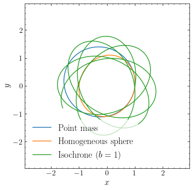
The green rosette orbit in the isochrone potential does not close.
To see how the orbit moves along this rosette pattern, we generate an animation of the rosette orbit using oi.animate() (the following integrates for ten radial periods):
To get a sense of how the rosette pattern changes as one goes from the Keplerian limit (\(b \approx 0\)) to the homogeneous-density limit (\(b \rightarrow \infty\)), the following interactive figure shows an orbit with the same initial condition for different values of \(b\). Drag the slider (slowly, because these orbits are computed on-the-fly by your browser) or use the buttons to see how the rosette pattern develops (the slider/buttons increase \(b\) logarithmically close to the limits and linearly in between).
For \(b\) near zero, the rosette manifests as a precession of the orbit, but as \(b\) increases, a clear rosette pattern appears. Once \(b\) gets to \(b \gg r\), the \(\Delta \psi \rightarrow \pi\) behavior makes subsequent orbits bunch up again and eventually the orbit closes for very large \(b\).
To demonstrate that orbits of the same energy have the same radial period, even though their differing angular momenta can cause them to have quite different orbits, let’s integrate two quite eccentric orbits in an isochrone potential that have the same specific energy, but different angular momenta. The first orbit starts at its apocenter, the second at its pericenter. We also integrate circular orbits at these apo- and pericenter radii to make it clear when each orbit has gone through a radial period:
[61]:
ip= potential.IsochronePotential(normalize=1.,b=0.4)
o1= Orbit([1.,0.,ip.vcirc(1.)-0.7,0.])
os= Orbit([[1.,0.,ip.vcirc(1.)-0.7,0.],
          [0.4,0.,numpy.sqrt(2.*(o1.E(pot=ip)-ip(0.4,0.))),0.],
          [1.,0.,ip.vcirc(1.),0.], # also animate circular orbits at apo/pericenter
          [0.4,0.,ip.vcirc(0.4),0.]])
Tr= o1.Tr(pot=ip)
ts= numpy.linspace(0.,3*Tr,501)
os.integrate(ts,ip)
os.animate(d1=['t','x'],d2=['r','y'],staticPlot=True); # remove the ; to display the animation
We see that whenever the blue orbit reaches its apocenter (the green line/circle), the orange orbit reaches its own pericenter (the red line/circle). Thus, their radial periods are the same. However, even though they both start at \(\psi = 0\), at the end of the three displayed radial periods, their azimuthl angle is clearly different (about \(3\pi/2\) for the orange orbit and a little less for the blue orbit), which is due to their different angular momentum.
To illustrate that this behavior is generic (but not exact), let’s consider the same orbits in the spherical NFW potential that represents the dark-matter halo in galpy’s MWPotential2014 model for the Milky Way’s gravitational field. To keep the orbits similar to those in the isochrone example above, we normalize the NFW model also such that \(v_c(r=1) = 1\).
[68]:
from galpy.potential import MWPotential2014
hp= MWPotential2014[2]
# Note that this normalization alters MWPotential2014, so don't do this
# if you still want access to MWPotential2014 in the same Python session
hp.normalize(1.)
o1= Orbit([1.,0.,hp.vcirc(1.)-0.7,0.])
os= Orbit([[1.,0.,hp.vcirc(1.)-0.7,0.],
          [0.4,0.,numpy.sqrt(2.*(o1.E(pot=hp)-hp(0.4,0.))),0.],
          [1.,0.,hp.vcirc(1.),0.], # also animate circular orbits at apo/pericenter
          [0.4,0.,hp.vcirc(0.4),0.]])
Tr= o1.Tr(pot=hp)
ts= numpy.linspace(0.,3*Tr,501)
os.integrate(ts,hp)
os.animate(width=600,d1=['t','x'],d2=['r','y'],staticPlot=True);
It is clear that the radial period of the two orbits is still approximately equal (there is only a small difference after three radial periods of the blue orbit), illustrating that the angular momentum is a minor contributor to the difference in radial period between orbits.
5.3. Integrals of motion
We end our first dive into the properties of galactic orbits by discussing integrals of motion. An integral of motion is any quantity \(I(\vec{x},\vec{v})\) that only depends on the current phase-space position \((\vec{x},\vec{v})\) (and not on the time) that is conserved along the orbit:
for all pairs \((\vec{x}_1,\vec{v}_1)\) and \((\vec{x}_2,\vec{v}_2)\) along the same orbit.
We have already encountered a few quantities that have this property. In Section 5.1 above, we proved that the specific angular momentum vector \(\vec{L}\) is conserved along each orbit in a spherical potential and because \(\vec{L} = \vec{x}\times\vec{v}\) it satisfies Equation \eqref{eq-spherorb-intmotion-definition}. Thus, each orbit in a spherical mass distribution has at least three integrals of motion: the three components of the angular momentum. In Chapter 4.1, we showed that the specific energy \(E\) is conserved for any static potential (whether spherical or not; Equation 4.14). Because for a static potential, \(E = |\vec{v}|^2/2 + \Phi(x)\), it also satisfies Equation \eqref{eq-spherorb-intmotion-definition} and is therefore an integral of motion. Orbits in static spherical potentials therefore have at least four integrals of motion: the specific energy and the three components of the angular momentum.
Integrals of motion like the specific energy and angular momentum are of high importance in the study of galactic orbits and of galactic equilibria, because they are isolating integrals. This means that these integrals restrict the orbit to a sub-space (typical of lower dimensionality) of the full phase-space volume that they would otherwise have access to. For example, in a static, spherical mass distribution, an orbit could in principle reach all of the six-dimensional phase space, but as we demonstrated in Section 5.1, the conservation of the direction of the angular momentum limits the orbit to a two-dimensional plane in configuration space, or a four-dimensional sub-space of the full phase space. Within this four-dimensional sub-space, the conservation of the magnitude of the angular momentum (the remaining component after accounting for two for the direction) restricts the orbit further to the three-dimensional sub-space where the angular velocity is determined by the radius through \(\dot{\psi} = L/r^2\) (Equation \ref{eq-eom-spher-angle}). Finally, energy conservation relates the radial velocity \(\dot{r}\) to the radius as well through Equation \eqref{eq-energy-spherpot}. Most spherical potentials do not have any further, independent isolating integrals of motion and orbits can explore the full two-dimensional area in \((r,\psi)\) at \(r_p \leq r \leq r_a\).
While when one thinks of integrals of motion, one typically thinks of such quantities as “angular momentum” or “energy”, but as soon as an orbit has one integral of motion, the orbit in fact has infinitely many of them. This is because any function \(f(I)\) of one or more integrals of motion is itself an integral of motion (it is easy to see that Equation \ref{eq-spherorb-intmotion-definition} holds for any function of \(I\)). Such a function can be explicit or implicit. For example, we have introduced the peri- and apocenter radius in a static, spherical potential in Section 5.1 and because these are implicitly defined as the solution of Equation \eqref{eq-spherpot-drdt}, which otherwise only depends on \(E\) and \(L\), they are also conserved and they can be computed based on the current phase-space position alone. So the peri- and apocenter radii are also integrals of motion. Similarly, one could use the radius of a circular orbit with specific angular momentum \(L\) (the radius \(r_L\) such that \(L = r_L\,v_c(r_L)\); again an implicit definition, in terms of \(L\) alone this time). Another useful alternative set of integrals of motion are the actions that we discussed in Chapter 4.4.3, because they are in many ways the natural coordinates to use when studying orbits and galactic equilibria. All of these alternative integrals of motion are in fact useful when using integrals of motion to build models of galaxies. However, keep in mind that such integrals of motion that are fully degenerate with other integrals of motion do not lead to additional restrictions on the phase-space volume covered by an orbit (even though they can be isolating integrals as well). We will refer to a set of integrals of motion where no individual integral can be computed solely based on the others as a set of independent integrals of motion.
The angular momentum is in fact a bit of a special set of integrals of motion even among other isolating integrals of motion. The reason for this is that the spherical symmetry of the mass distribution associated with the angular momentum allows the Hamilton-Jacobi equation that we discussed in Chapter 4.4.3 to be simplified (and in fact solved) through the technique of separation of variables and Hamilton’s characteristic function can be written as \(W(r,\theta,\phi;\vec{C}) = W_r(r;\vec{C})+W_\theta(\theta;\vec{C})+W_\phi(\phi;\vec{C})\). What this means in practice is that the motion becomes explicitly the combination of three oscillations: a first trivial one of the orbit’s position with respect to the plane perpendicular to the angular-momentum vector (trivial, because the oscillation amplitude is zero, as the orbit does not leave this plane), a second one in \(\psi\) with dynamics \(\dot{\psi} = L/r^2\) that couples to the third oscillation in \(r\) determined by the effective potential \(\Phi_\mathrm{eff}(r;L)\). Thus, the conservation of the angular momentum does not only restrict the orbit to lie within a three-dimensional subspace of six-dimensional phase-space, it is also directly responsible for the fact that the orbit can be described as a simple \(r\) oscillation in the effective potential, and an \(r\)-dependent \(\phi\) oscillation. When one actually solves the Hamilton-Jacobi relation, one finds that two components of the angular momentum vector are in fact actions (see Chapter 4.4.3; the third component of the angular momentum is not an action, but instead related to one of the angles in the action-angle formalism, which is constant for spherical mass distributions rather than increasing linearly as usual). We will see that the conservation of the \(z\)-component of the angular momentum in axisymmetric potentials has a similar simplifying effect. Without this special property, the study of galactic orbits would be significantly harder!
We discussed Noether’s theorem in Chapter 4.3, which states that if a system has a continuous symmetry property, then there are corresponding quantities whose values are conserved in time. By Noether’s theorem, a continuous symmetry property results in an integral of motion. However, the opposite direction of this implication does not hold in any useful manner: just because a system has an integral of motion, does not mean that it necessarily has a corresponding continuous symmetry property that is in any way useful (given any integral of motion, it is possible to define a convoluted symmetry using Hamiltonian mechanics). For example, when we discuss orbits in static, axisymmetric disks, we will see that such orbits appear to have an exact integral of motion in addition to the specific energy and \(z\)-component of the angular momentum, but this integral cannot be calculated from an analytical expression in general and does not correspond to a simple symmetry property of the system.
Regular orbits (Chapter 4.4.3) in general mass distributions typically have three independent integrals of the motion, but not more. Orbits in static spherical potentials are therefore special because they have at least four independent integrals of motion: the three components of the angular momentum and the specific energy. Physically, the additional integral of motion causes one of the oscillations that regular orbits normally have, the oscillation of the orbit with respect to the average orbital plane, to vanish (in the language of action-angle coordinates, this means that the frequency of that oscillation is exactly zero and the angle associated with it is a conserved quantity as well). Orbits in the point-mass and homogeneous-sphere mass distributions that we discussed above, actually have an additional, fifth integral of the motion. This fifth integral of motion is responsible for the fact that the orbits in these mass distributions close and form ellipses, thus requiring only a single variable that is a function of \((\vec{x},\vec{v}\) to describe where a body is along the orbit (for Keplerian orbits, this is, e.g., the true or eccentric anomaly). For Keplerian orbits, this fifth integral of the motion is typically taken to be the Laplace–Runge–Lenz vector. But for both the point-mass and homogeneous-sphere potential, it can be taken to be the unit vector in the orbital plane (thus, only requiring a single number to specify) that points to the pericenter (at \(x\geq 0\) for the homogeneous sphere). For general spherical potentials, this vector is not conserved, because the azimuth of the pericenter changes from radial period to radial period, but for the point-mass and homogeneous-sphere potentials, the pericenter remains fixed in place for all time.
We will often use spherical mass distributions, and even the point-mass potential, as approximations of galactic mass distributions, because their simple properties make them so much easier to deal with. However, the fact that orbits in spherical potentials have more independent integrals of motion than orbits in more realistic galactic mass distributions is something to remain vigilant about when doing this. For example, in problems where any motion perpendicular to the average orbital plane is important, the fact that this motion is zero for spherical potentials renders them inapplicable to studying these problems. Similarly, Keplerian orbits are sometimes a nice approximation to make, because they are known analytically and are quite simple. But when one, for example, studies how a population of stars fills the entire volume of phase space allowed by its integrals of motion, the fact that Keplerian orbits only fill a one-dimensional sub-space, rather than the three-dimensional one of typical regular orbits, can trick one into making incorrect inferences and predictions about this process.