← Previous section Next section →

8.2. Rotation curves of external galaxies

\label{sec-galrot-velfield-extgals}

In the previous section, we described two-dimensional velocity fields of external galaxies and how features in these fields relate to the underlying rotation of the galaxy. Now that we understand the basic structure of two-dimensional velocity fields, we can focus our attention on how we can determine the one-dimensional rotation curve from these fields and how we can use it to determine the mass distribution of galaxies and find convincing evidence of the existence of dark matter.

8.2.1. From velocity fields to rotation curves

\label{sec-galrot-velfield-to-rotcurve}

There are various methods for extracting the one-dimensional rotation curve \(v_c(R)\) of a galaxy from a map of its two-dimensional velocity field \(V(x,y)\). The simplest of these uses the fact that \(V(x,0) = \mathrm{sign(x)}\,v_c(R)\,\sin i\) and therefore \begin{equation}\label{eq-vc-from-vxy-simple} v_c(R) = \frac{V(x,0)}{\sin i\,\mathrm{sign(x)}}\,. \end{equation} If we have actually determined the two-dimensional field \(V(x,y)\), then this method throws out much information, but as we have discussed, many observations—especially using optical spectroscopy—only determine \(V(x,0)\), not the full two-dimensional field \(V(x,y)\). Using Equation (8.9) is then the only option to extract the rotation curve. The galaxy’s inclination needs to be known from photometric observations, because otherwise it is degenerate with \(v_c(R)\). One simple way to estimate the inclination for a disk galaxy is to assume that its face-on shape is circular, such that the elliptical shape of observed isophotes is solely due to the inclination’s projection effect.

When we have measured the full 2D \(V(x,y)\) field, we can use Equation (8.2) and fit for the free parameters. This typically includes the center of the galaxy on the sky \((x_0,y_0)\) (which we have set to \((0,0)\) in the discussion so far), the angle \(\phi_0\) of the galaxy’s major axis at the receding-velocity side, typically measured counter-clockwise from the north (which we set to \(\phi_0 = 180^\circ\) above), the systemic velocity of the galaxy \(V_0\) (which we set to zero above), the inclination \(i\) if not fixed by photometric observations, and parameters describing \(v_c(R)\). A popular method for performing the fit is to perform it in a set of annuli around the center of the galaxy, where each annulus can in principle have its own value for all of the parameters that we mentioned. Because the annuli can be tilted with respect to each other when they have different \((i,\phi_0)\), this method is known as the tilted-ring model (e.g., Begeman 1989). To account for any deviations from circular rotation, these fits also often include a radial term \(v_r(R)\) to model radial motions in the plane.

Including all parameters, the observed velocity field is given by \begin{equation} V(x,y) = V_0 + v_c(R)\,\cos\theta\,\sin i + v_r(R)\,\sin\theta\,\sin i\,, \end{equation} where \begin{align} \cos \theta& = \frac{-(x-x_0)\,\sin \phi_0+(y-y_0)\,\cos \phi_0}{R}\,,\\ \sin \theta& = \frac{-(x-x_0)\,\cos \phi_0-(y-y_0)\,\sin \phi_0}{R\,\cos i}\,. \end{align} In practice, parameters such as \((x_0,y_0)\) are typically fixed to be (i) the same for each tilted ring and (ii) determined by the photometric center.

8.2.2. Observed rotation curves

\label{sec-galrot-obsrotcurves}

Now that we know how to extract rotation curves from observed velocity fields, let us look at some classical results on rotation curves. We start by looking at the rotation curves derived from the one-dimensional velocity fields from Rubin et al. (1980) shown in Figure 8.1. The rotation curves of these and other galaxies are displayed in Figure 8.7.

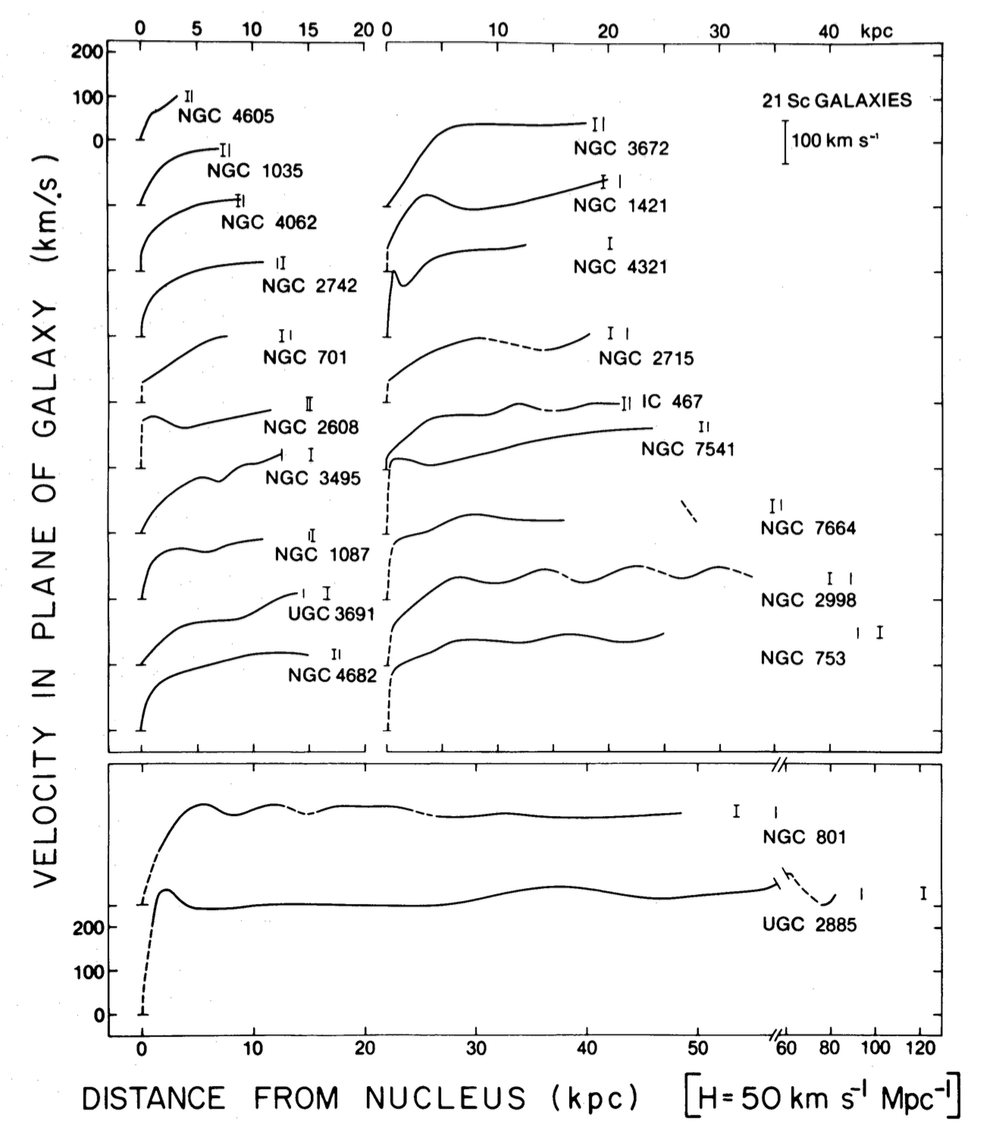
Figure 8.7: Observed rotation curves for Sc galaxies (Rubin et al. 1980).

The vertical line segments in this figure are the so-called optical radius \(R_{25}\), which is defined as the radius corresponding to the isophote where the surface brightness is \(25\,\mathrm{mag\,arcsec}^{-2}\). This is a convenient definition of the radius of a galaxy’s light, because galaxies emit little light outside of this radius. Most of the rotation curves do not reach the optical radius, but they typically get close. We would therefore expect to see the rotation curve turn over if these disk galaxies were pure exponential disks. However, the rotation curves remain mostly flat at the largest observed radius.

Kent (1986) obtained photometry for these galaxies and asked the question: can these rotation curves be fit with constant mass-to-light ratios and are the mass-to-light ratios reasonable considering our knowledge of stellar population from which we expect mass-to-light ratios of a few (see also Kalnajs 1983). To answer this question, Kent (1986) measured the surface-brightness profile \(\mu(R)\) of these galaxies and decomposed them into a bulge \(\mu_b(R)\) and a disk \(\mu_d(R)\) component, each of which is allowed to have a different constant mass-to-light ratio, \((M/L)_b\) and \((M/L)_d\), respectively. The total surface density is then \begin{align} \Sigma(R) & = \Sigma_b(R) + \Sigma_d(R)= (M/L)_b\,\mu_b(R) + (M/L)_d\,\mu_d(R)\,. \end{align} We can use the framework from the previous chapter to determine the circular velocity profile \(v_c(R)\) corresponding to this surface density profile.

For the bulge, we may assume that the underlying mass distribution is spherical. We then first need to deproject the observed surface-density profile, using the inversion equation (6.17) to obtain the luminosity density \(\nu_b(r)\) \begin{equation} \nu_b(r) = -\frac{1}{\pi}\,\int_r^\infty\mathrm{d}R\,\frac{\mathrm{d} \mu(R)}{\mathrm{d} R}\,\frac{1}{\sqrt{R^2-r^2}}\,. \end{equation} and then integrate this to obtain the enclosed luminosity profile \((L_b(<r)\) \begin{equation}\label{eq-bulge-enc-lum-kent} L_b(< r) = 4\pi\,\int_0^r\,\mathrm{d}s\,s^2\,\nu_b(s)\,. \end{equation} The circular velocity from the bulge component is then simply given by \begin{equation}\label{eq-vcb-kent} v_{c,b}^2(r) = \left(\frac{M}{L}\right)_b\,\frac{G\,L_b(< r)}{r}\,. \end{equation}

To obtain the contribution of the disk component \(v_{c,d}^2(r)\), we start with the expression for the circular velocity of a razor-thin disk as a function of the surface density from Equation (7.35). We can write this equation in a more convenient form for applying to an arbitrary \(\Sigma_d = (M/L)_d\,\,\mu_d(R)\) as \begin{align} v_{c,d}^2(R) & =2\pi\,G\,R\,(M/L)_d\,\int_0^\infty \mathrm{d} R'\,R'\,\mu_d(R')\,\int_0^\infty\mathrm{d}k\,\,J_1(kR)\,k\, \,J_0(kR')\nonumber\\ & =-2\pi\,G\,R\,(M/L)_d\,\int_0^\infty \mathrm{d} R'\,R'\,\mu_d(R')\,\frac{\mathrm{d}}{\mathrm{d}R}\left[\int_0^\infty\mathrm{d}k\,\,J_0(kR)\,\,J_0(kR')\right]\, \end{align} The integral in square brackets is a simpler version of an integral that we encountered in Equation (7.38), which we can also write as \begin{equation} \int_0^\infty\mathrm{d}k\,J_0(kR) \,J_0(kR') = \frac{2}{\pi}\begin{cases}\frac{1}{R}\,\,K\left(\left[\frac{R'}{R}\right]^2\right) & R' < R\\ \frac{1}{R'}\,\,K\left(\left[\frac{R}{R'}\right]^2\right) & R' < R\\\end{cases}\,, \end{equation} where \(K(m)\) is the complete elliptic integral of the first kind. Therefore, \begin{align} v_{c,d}^2(R) & = 4\,G\,(M/L)_d\,\Bigg\{ \int_0^R \mathrm{d} R'\,\mu_d(R')\frac{R'}{R}\,\frac{E(m)}{(1-m)}+ \int_R^\infty \mathrm{d} R'\,\mu_d(R')\,\left[K(m^{-1})-\frac{E(m^{-1})}{1-m^{-1}}\right]\Bigg\}\,,\label{eq-vcd-kent} \end{align} where \(m=(R'/R)^2\). This integral—which has an integrable singularity at \(R = R'\), so some care needs to be taken in its numerical calculation—allows us to compute the rotation curve for any razor-thin disk \(\Sigma_d(R) = (M/L)_d\,\mu_d(R)\). For a given \(\mu_d(R)\), we can compute the function in the curly brackets once and then adjust the mass-to-light ratio \((M/L)_d\) to change \(v_{c,d}^2(R)\). We could have also derived this expression for the circular velocity by starting from the general expression for the gravitational potential of any axisymmetric, razor-thin disk in Equation (7.55).

By combining Equations (8.16) and (8.19), we can then compute the rotation curve corresponding to the observed bulge and disk surface brightness for different values of \((M/L)_b\) and \((M/L)_d\). We can then ask whether we can fit the entire rotation curve if we adjust the mass-to-light ratios such that they provide a good fit to the rotation curve in the inner region. These are known as maximum-disk fits, because we set the mass-to-light ratios to the largest possible value—any larger and the computed inner rotation curve would be larger than the observed one. Kent (1986) did this for many galaxies. Figure 8.8 shows the result for two of them that demonstrates the two different situations that occur.

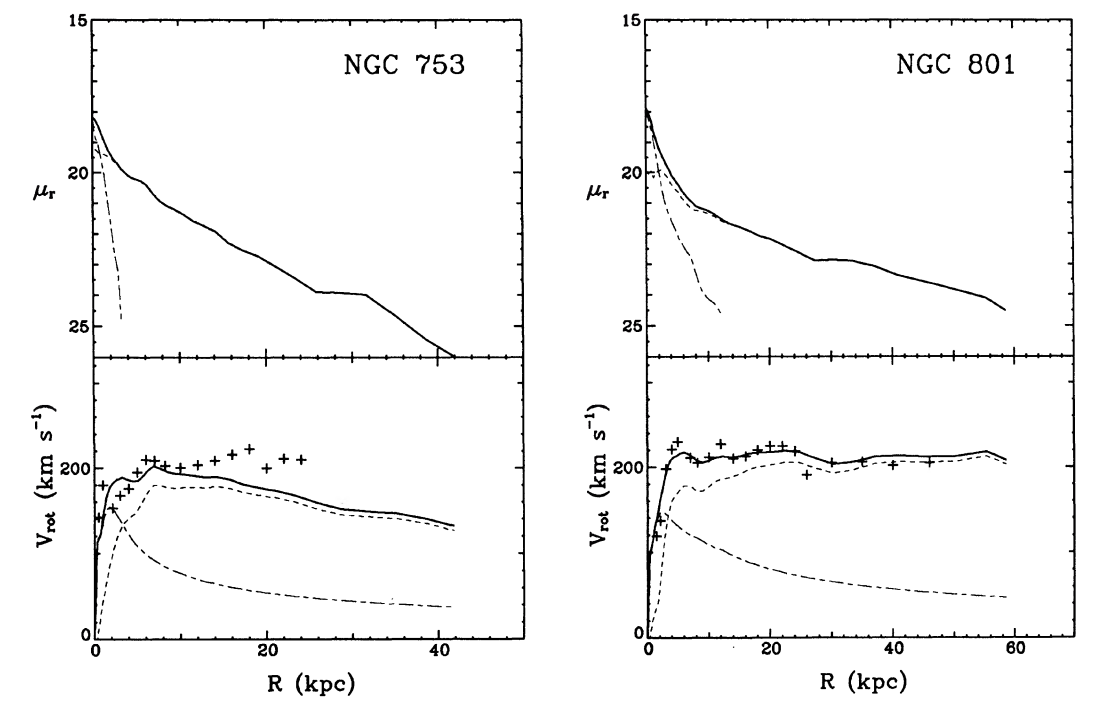
Figure 8.8: Maximum-disk fits to galaxy surface brightnesses (top) and rotation curves (bottom). Note that \(\mu(R)\) in this figure is the surface brightness expressed in logarithmic units \(\mathrm{mag\,arcsec}^{-2}\). From Kent (1986).

These figures display the observed surface-brightness profile \(\mu(R)\) and its decomposition into bulge \(\mu_b(R)\) and disk \(\mu_d(R)\) components in the top panel. The bottom panels show the observed rotation curve and the maximum-disk fits described above.

We see that in the case of NGC 801 the maximum-disk fit provides an excellent match to the entire observed rotation curve, even though the rotation curve extends to 50 kpc. Thus, there appears to be no need for additional matter. The NGC 801 fit has \((M/L)_b \approx 1.5\) and \((M/L)_d \approx 7\); the maximum-disk fit therefore requires a somewhat high mass-to-light ratio. But nevertheless, it is remarkable that NGC 801’s rotation curve and surface brightness can be fit without including any halo dark matter (at least for the data available in 1986, see below).

NGC 753, however, displays very different behavior. The maximum-disk fit successfully reproduces the inner (\(R \lesssim 10\,\mathrm{kpc}\)) rotation curve, but because the surface-brightness profile steeply declines at large radii, the maximum-disk rotation curve drops at \(R \gtrsim 10\,\mathrm{kpc}\). The observed rotation curve, however, remains approximately constant. The mass-to-light ratios for NGC 753’s maximum-disk fit are reasonable: \((M/L)_b \approx 3\) and \((M/L)_d \approx 1.2\). Therefore, it is clear that we need an additional component to explain NGC 753’s rotation curve. Equivalently, the mass-to-light ratio needs to increase with \(R\).

It is instructive to look through the other fits in the Kent (1986) paper. Most of the galaxies considered behave similar to NGC 801: the maximum-disk rotation curve can explain the entire observed rotation curve, except for perhaps the last few points. This demonstrates the difficulty in using optical rotation curves to constrain the mass-to-light ratio in the outer regions of galaxies: these curves typically do not extend far enough to unambiguously show the influence of dark matter.

We can repeat Kent (1986)’s analysis using more modern data. The SPARC (Spitzer Photometry and Accurate Rotation Curves) sample of Lelli et al. (2016a) consists of 175 nearby galaxies with mid-infrared photometry photometry from the Spitzer space telescope (at \(3.6\,\mu\mathrm{m}\)) and precise rotation curves from 21cm and H\(\alpha\) observations.

To use this data here, we first implement a general function to download the data from Vizier, which we will also use elsewhere:

# vizier.py: download catalogs from Vizier
import sys
from pathlib import Path
import shutil
import tempfile
from ftplib import FTP
import subprocess
_ERASESTR= "                                                                                "
def vizier(cat,filePath,ReadMePath,
           catalogname='catalog.dat',readmename='ReadMe'):
    """
    NAME:
       vizier
    PURPOSE:
       download a catalog and its associated ReadMe from Vizier
    INPUT:
       cat - name of the catalog (e.g., 'III/272' for RAVE, or J/A+A/... for journal-specific catalogs)
       filePath - path of the file where you want to store the catalog (note: you need to keep the name of the file the same as the catalogname to be able to read the file with astropy.io.ascii)
       ReadMePath - path of the file where you want to store the ReadMe file
       catalogname= (catalog.dat) name of the catalog on the Vizier server
       readmename= (ReadMe) name of the ReadMe file on the Vizier server
    OUTPUT:
       (nothing, just downloads)
    HISTORY:
       2016-09-12 - Written as part of gaia_tools - Bovy (UofT)
       2017-09-12 - Copied to galdyncourse (yes, same day!) - Bovy (UofT)
       2019-12-20 - Copied directly into notes to avoid additional dependency - Bovy (UofT)
    """
    _download_file_vizier(cat,filePath,catalogname=catalogname)
    _download_file_vizier(cat,ReadMePath,catalogname=readmename)
    catfilename= Path(catalogname).name
    with open(ReadMePath,'r') as readmefile:
        fullreadme= ''.join(readmefile.readlines())
        if catfilename.endswith('.gz') and not catfilename in fullreadme:
            # Need to gunzip the catalog
            try:
                subprocess.check_call(['gunzip',filePath])
            except subprocess.CalledProcessError as e:
                print("Could not unzip catalog %s" % filePath)
                raise
    return None

def _download_file_vizier(cat,filePath,catalogname='catalog.dat'):
    sys.stdout.write('\r'+"Downloading file %s from Vizier ...\r" \
                         % (Path(filePath).name))
    sys.stdout.flush()
    try:
        # make all intermediate directories
        os.makedirs(Path(filePath).parent)
    except OSError: pass
    # Safe way of downloading
    downloading= True
    interrupted= False
    file, tmp_savefilename= tempfile.mkstemp()
    os.close(file) #Easier this way
    ntries= 1
    while downloading:
        try:
            ftp= FTP('cdsarc.u-strasbg.fr')
            ftp.login()
            ftp.cwd(str(Path('pub') / 'cats' / cat))
            with open(tmp_savefilename,'wb') as savefile:
                ftp.retrbinary('RETR %s' % catalogname,savefile.write)
            shutil.move(tmp_savefilename,filePath)
            downloading= False
            if interrupted:
                raise KeyboardInterrupt
        except:
            if not downloading: #Assume KeyboardInterrupt
                raise
            elif ntries > 5:
                raise IOError('File %s does not appear to exist on the server ...' % (Path(filePath).name))
        finally:
            if Path(tmp_savefilename).exists():
                os.remove(tmp_savefilename)
        ntries+= 1
    sys.stdout.write('\r'+_ERASESTR+'\r')
    sys.stdout.flush()
    return None

We then write a function to download the SPARC data and store it in a cache directory $HOME/.galaxiesbook/cache/vizier (this directory will be automatically created on your system):

import os
from pathlib import Path
from astropy.io import ascii
_CACHE_BASEDIR= Path(os.getenv('HOME')) / '.galaxiesbook' / 'cache'
_CACHE_VIZIER_DIR= _CACHE_BASEDIR / 'vizier'
_LELLI_VIZIER_NAME= 'J/AJ/152/157'
def download_sparc(verbose=False):
    """
    NAME:
       download_sparc
    PURPOSE:
       download and read the Lelli et al. (2016) catalog of
       rotation curves and photometry for galaxies
       in the SPARC sample
    INPUT:
       verbose= (False) if True, be verbose
    OUTPUT:
       pandas dataframe
    HISTORY:
       2021-01-05 - Written - Bovy (UofT)
    """
    # Generate file path and name
    tPath= _CACHE_VIZIER_DIR / 'cats'
    for directory in _LELLI_VIZIER_NAME.split('/'):
        tPath = tPath / directory
    filePath= tPath / 'table2.dat'
    readmePath= tPath / 'ReadMe'
    # download the file
    if not filePath.exists():
        vizier(_LELLI_VIZIER_NAME,filePath,readmePath,
               catalogname='table2.dat',readmename='ReadMe')
    # Read with astropy
    table= ascii.read(str(filePath),readme=str(readmePath),format='cds')
    return table.to_pandas()

and a function to read the data for a single galaxy:

def read_sparc_data(galaxy):
    """Return the data for a given galaxy"""
    raw= download_sparc()
    return raw[raw['Name'] == galaxy]

Then we write some functions to deal with the surface brightness profile. We will only deal with galaxies that only have a small bulge component and we will ignore this bulge component, instead assuming that the entire surface brightness is contributed by the disk (that is, in the notation above, we assume that \(\mu(R) = \mu_d(R)\) and \(v_c(R) = v_{c,d}(R)\)). This assumption only affects the rotation curve within the inner few kpc. The following function plots the surface brightness as a function of radius for a given galaxy:

import re
def plot_sparc_lumprofile(galaxy):
    data= read_sparc_data(galaxy)
    semilogy(data['Rad'],data['SBdisk'],
             marker='o',ls='none',color='k',zorder=1)
    xlim(0.,1.1*numpy.amax(data['Rad']))
    ylim(0.5**numpy.amax(data['SBdisk']),
         2*numpy.amax(data['SBdisk']))
    xlabel(r'$R\,(\mathrm{kpc})$')
    ylabel(r'$\mu\,(L_\odot\,\mathrm{pc}^{-2})$')
    galpy_plot.text(r'$\mathrm{{{}}}$'.format(
        '\\ '.join([s  if (len(s) < 2 or s[0] != '0')
                       else s[1:]
                       for s in re.split(r'(\d+)',galaxy)])),
                    size=18.,top_right=True)
    return [0.,1.1*numpy.amax(data['Rad'])]

Next we create a class to build a simple model for the surface brightness profile \(\mu(R)\): a cubic spline through the observed data points. We also implement a function to plot the model luminosity profile:

from scipy import interpolate
class model_lumprofile():
    # By 'lumprofile' we mean surface-brightness profile here
    def __init__(self,galaxy):
        data= read_sparc_data(galaxy)
        data= data[data['SBdisk'] > 0]
        self._Rmin= numpy.amin(data['Rad'])
        self._Rmax= numpy.amax(data['Rad'])
        self._lum_at_Rmin= numpy.array(data['SBdisk'])[numpy.argmin(data['Rad'])]
        self._ip= interpolate.InterpolatedUnivariateSpline(\
                    data['Rad'],numpy.log(data['SBdisk']),k=3)
    def __call__(self,R):
        Rinternal= numpy.atleast_1d(R)
        # We assume that mu(R) is zero beyond the last data point
        # and constant within the innermost data point
        out= numpy.zeros(Rinternal.shape)
        if isinstance(Rinternal,u.Quantity):
            Rinternal= Rinternal.to_value(u.kpc)
        oindx= (Rinternal >= self._Rmin)*(Rinternal <= self._Rmax)
        out[oindx]= numpy.exp(self._ip(Rinternal[oindx]))
        oindx= Rinternal < self._Rmin
        out[oindx]= self._lum_at_Rmin
        return out.reshape(R.shape)*u.Lsun/u.pc**2
def plot_model_lumprofile(RRange,lumprofile):
    Rs= numpy.linspace(RRange[0],RRange[1],101)
    plot(Rs,lumprofile(Rs),lw=2.,zorder=10)
    return None

Next, we define a function to plot the observed rotation curve:

def plot_sparc_rotcurve(galaxy):
    data= read_sparc_data(galaxy)
    errorbar(data['Rad'],data['Vobs'],yerr=data['e_Vobs'],
             marker='o',ls='none',color='k',zorder=1)
    xlim(0.,1.1*numpy.amax(data['Rad']))
    ylim(0.,1.3*numpy.amax(data['Vobs']))
    xlabel(r'$R\,(\mathrm{kpc})$')
    ylabel(r'$v_c\,(\mathrm{km\,s}^{-1})$')
    return [0.,1.1*numpy.amax(data['Rad'])]

With the model for the observed surface brightness profile from the SPARC database, we can use Equation (8.19) to turn this profile into a predicted rotation curve using a mass-to-light ratio \(M/L\). We can do this using galpy’s AnyAxisymmetricRazorThinDiskPotential, which implements Equation (8.19) (in fact, a more general version that includes the full potential and all its derivatives):

from galpy.potential import AnyAxisymmetricRazorThinDiskPotential
def model_diskpot(MoverL,lumprofile):
    return AnyAxisymmetricRazorThinDiskPotential(\
                surfdens=lambda R: MoverL*lumprofile((R/u.kpc).to_value(u.dimensionless_unscaled)),
                                                 ro=8.,vo=220.)
def plot_model_diskrotcurve(RRange,diskpot):
    Rs= numpy.linspace(RRange[0],RRange[1],101)
    plot(Rs,[diskpot.vcirc(R*u.kpc).to_value(u.km/u.s) for R in Rs],lw=2.,zorder=10)
    return None

Finally, we put everything together to plot the observed surface brightness profile and rotation curve for a galaxy and the model resulting from applying Equation (8.19) for an assumed mass-to-light ratio:

from matplotlib import gridspec
from matplotlib.ticker import FuncFormatter
def plot_sparc(galaxy,gs):
    subplot(gs(0))
    plot_sparc_lumprofile(galaxy)
    gca().yaxis.set_major_formatter(FuncFormatter(
                lambda y,pos: (r'${{:.{:1d}f}}$'.format(int(\
                    numpy.maximum(-numpy.log10(y),0)))).format(y)))
    gca().tick_params(labelbottom=False)
    subplot(gs(1))
    plot_sparc_rotcurve(galaxy)
    return None
def plot_sparc_model(MoverL,galaxy,gs):
    lumprofile= model_lumprofile(galaxy)
    subplot(gs(0))
    data= read_sparc_data(galaxy)
    model_RRange= [numpy.amin(data['Rad']),numpy.amax(data['Rad'])]
    plot_model_lumprofile(model_RRange,lumprofile)
    subplot(gs(1))
    diskpot= model_diskpot(MoverL,lumprofile)
    plot_model_diskrotcurve(model_RRange,diskpot)
    return None

Let's now look at some of the galaxies that Kent (1986) studied as well. NGC 753 is not part of the SPARC sample, but NGC 801 is, so we can revisit it. We’ll also look at NGC 2998. We choose a mass-to-light ratio that maximizes the disk contribution, by setting it as high as we can without predicting a circular velocity that is too much above the observed rotation curve in the inner galaxy (we allow the prediction to be a bit high in the inner ten kpc, because we are ignoring the bulge, which would predict a smaller rotation velocity for the same surface brightness). The result is shown in Figure 8.9.

figure(figsize=(8,5.5))
gs= gridspec.GridSpec(ncols=2,nrows=2,hspace=0.,
                     height_ratios=[2,1])
plot_sparc('NGC2998',lambda i: gs[i,0])
plot_sparc_model(0.9*u.Msun/u.Lsun,'NGC2998',lambda i: gs[i,0])
plot_sparc('NGC0801',lambda i: gs[i,1])
plot_sparc_model(0.6*u.Msun/u.Lsun,'NGC0801',lambda i: gs[i,1])
tight_layout();

Figure 8.9: Maximum-disk fits to galaxy surface brightnesses (top) and rotation curves (bottom) from the SPARC database.

We see that in both cases, the predicted rotation curve for the maximum-disk fit peaks at 5 to 10 kpc from the center and then decays to a value that is just over half of the observed value at the largest radius. We also see that the predicted disk rotation curve for NGC 801 decays rather than staying flat in the Kent (1986) analysis. This is because the more accurate and precise Spitzer photometry displays a steeper decline than the photometry used by Kent (1986). The mass-to-light ratios of \(M/L \approx 1\) are reasonable for the mid-infrared photometric bandpass used by SPARC.

Thus, we see that the combination of the modern photometric and rotation curve data for the disk galaxies observed by Rubin et al. (1980) clearly indicate that the mass-to-light ratio increases significantly with radius (by a factor of approximately four for the galaxies that we looked at).

Radio observations of the 21cm line of neutral hydrogen allow the velocity field to be mapped at larger distances than the optical rotation curves that we have discussed so far. In Figure 8.2, we showed the velocity maps from Bosma (1978) (which surely must be one of the most highly-cited PhD theses in astronomy). Many of these extend to beyond the optical radius of the galaxy, typically to between the optical radius and twice that radius. Therefore, we expect to approach the Keplerian drop-off in the rotation curves in the outer observed regions and we should see clear closed contours in the two-dimensional velocity maps \(V(x,y)\). However, looking at the velocity maps, we see that closed contours are rare and that most of the galaxies in Bosma’s sample have the “spider” shape indicative of flat rotation curves.

Bosma used a tilted-ring model to extract the one-dimensional rotation curves from the two-dimensional velocity fields. Figure 8.10 displays the resulting rotation curves, arranged by Hubble type (the “Galaxy” rotation curve is that of the Milky Way, which we will come back to below).

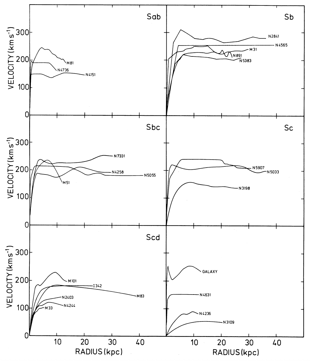
Figure 8.10: 21cm rotation curves for different galaxy types (Bosma 1978).

The rotation curves of the majority of these galaxies remain flat to the furthest observed point, typically well beyond the optical radius of the galaxy. While Bosma (1978) obtained some plate-based photometry, without good CCD-based optical photometry for these galaxies, Bosma (1978) could not do an analysis of the type and quality as performed by Kent (1986) for the Rubin et al. (1980) sample. Instead, Bosma (1978) attempted an inversion of the observed \(v_c(R)\) to \(\Sigma(R)\) and \(M(<R)\) assuming either (i) that the mass was distributed as a razor-thin disk with a to-be-determined surface density \(\Sigma(R)\) or (ii) that the mass was made up of spheroidal and simple disk components with to-be-determined parameters. The first of these methods is problematic, because determining a razor-thin disk’s \(\Sigma(R')\) at a radius \(R'\) requires knowledge of \(v_c(R)\) at large \(R\), but the rotation curves are observed to be flat at all \(R\), so extrapolating to the necessary decline at large \(R\) is difficult. However, no matter what method is used to determine \(M(<R)\) from the observed rotation curve, mass profiles similar to Bosma (1978)’s would result. Bosma (1978) found that \(M(<R) \propto R\), as expected from our discussion in Chapter 2.3. These galaxies have large masses enclosed within the radius of the last point where \(v_c(R)\) was measured and the mass should be expected to keep rising, because the increase barely flattens at large radius. The total masses obtained by Bosma (1978) are larger by a factor of at least a few than the mass observed within the optical radius and these radio observations therefore left no doubt about the presence of a large amount of dark matter in these galaxies.

Finally, let’s look at one of the best poster children for flat rotation curves: NGC 3198. We displayed the two-dimensional velocity field \(V(x,y)\) from the THINGS survey in Figure 8.3. That velocity field beautifully shows the vertical contours near the center (perpendicular to the major axis) indicative of solid-body rotation and the spider-like contours outside of the center indicative of a flat rotation curve. A tilted-ring analysis leads to the rotation curve for NGC 3198 shown in Figure 8.11.

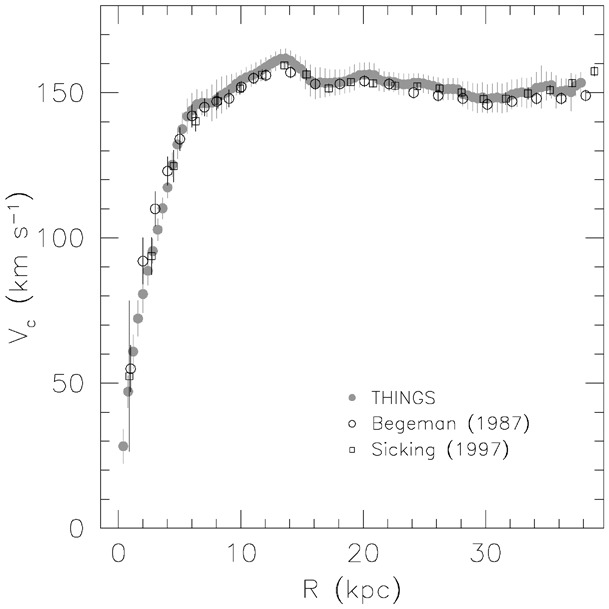
Figure 8.11: Quintessentially-flat rotation curve of NGC 3198 (de Blok et al. 2008).

The scale length of the light profile of NGC 3198 is \(\approx 2.7\,\mathrm{kpc}\) (van Albada et al. 1985) and the optical radius is about 10 kpc. This rotation curve therefore extends out to about 11 disk scale lengths or four times the optical radius. Looking at the rotation curve of an exponential disk in Chapter 7.3.3.2, we see that at 11 disk scale lengths the rotation velocity should be less than half of the maximum rotation velocity and we should see a strong decline in the rotation velocity that is essentially Keplerian. That the actual rotation curve is flat means that NGC 3198 must have a large amount of matter beyond the optical radius: approximately four times as much (van Albada et al. 1985). This is confirmed by repeating our Kent (1986)-style analysis using the SPARC data. For a mid-infrared mass-to-light ratio of \(M/L = 0.8\), we find the result in Figure 8.12.

figure(figsize=(5,7))
gs= gridspec.GridSpec(ncols=1,nrows=2,hspace=0.,height_ratios=[2,1])
plot_sparc('NGC3198',lambda i: gs[i,0])
plot_sparc_model(0.8*u.Msun/u.Lsun,'NGC3198',lambda i: gs[i,0])

Figure 8.12: Like Figure 8.9, but using SPARC data for NGC 3198.

Because the surface brightness profile is so close to exponential with a scale length of \(\approx 2.7\) kpc, we see that the rotation curve peaks at \(R \approx 6\) kpc as expected for an exponential disk (which peaks at \(R \approx 2.15\,R_d\), see Equation 7.49). The rotation curve predicted from the stellar luminosity alone then steadily declines and the mass-to-light ratio must increase with radius to counter-act this predicted decline for a constant mass-to-light ratio.

Thus, we see that the evidence from HI rotation curves of external galaxies is clear: galaxies must be surrounded by an extended distribution of non-luminous, dark matter that causes the total mass-to-light ratio to increase with radius.

← Previous section Next section →