
16.1. Supermassive black holes at the centers of galaxies
One of the great discoveries of the second half of the 1990s (aside from cosmic acceleration) is the fact that every massive galaxy has a supermassive black hole at its center. This field developed extraordinarily quickly, going from tentative evidence to full acceptance and statistical studies in just five years. Kormendy & Richstone (1995) summarized the tentative detections of eight supermassive black holes in 1995: starting with the first observations and a simple analysis using spherical and isotropic models of a central black hole in M87 (Sargent et al. 1978; Young et al. 1978; eventually confirmed with gas kinematics by Harms et al. 1994), the field had slowly developed over almost twenty years to eight tentative detections. Six of these were made by dynamical modeling of stellar kinematics, while two came from the more complex modeling of gas kinematics. By using two-integral axisymmetric modeling and three-integral Schwarzschild modeling (e.g., Magorrian et al. 1998; van der Marel et al. 1998; Cretton & van den Bosch 1999; Gebhardt et al. 2003) of observations using the Hubble Space Telescope (HST), evidence for central mass concentrations became highly secure by the year 2000 (we’ll refer to these as supermassive black holes, for some reason usually abbreviated as SMBHs). HST observations were crucial for this: the increased spatial resolution that was possible with HST was necessary to properly resolve the inner dynamical structure and rule out less dense central mass concentrations. This allowed for the demographics of the SMBH population as well as correlations between the SMBH mass and galaxy properties to be determined (e.g., Ferrarese & Merritt 2000; Gebhardt et al. 2000a). The connection between SMBHs and their galaxy has proven to be fertile ground for studying galaxy evolution that continues into the present day. In this section, we briefly discuss the dynamical evidence for SMBHs obtained using the dynamical-modeling techniques that we discussed in parts two and three.
The presence of SMBHs at the centers of galaxies can be detected with a large variety of techniques. In the low-redshift Universe, these are mainly (i) spectroscopic and astrometric observations of the stars near the Milky Way’s SMBH (see below), (ii) water megamasers (e.g., Miyoshi et al. 1995), (iii) gas kinematics traced using emission-line kinematics (e.g., Harms et al. 1994), and (iv) stellar kinematics combining photometry and absorption-line kinematics. For SMBHs that are active, that is, that accrete matter at a high enough rate to show up as active galactic nuclei or quasars (see Chapter 18.3), other techniques such as the properties of the fluorescent Fe K\(\alpha\) line (Reynolds & Nowak 2003) and reverberation mapping (Blandford & McKee 1982) are possible. We’ll focus here on the evidence coming from stellar kinematics, because it was crucial in establishing the presence of SMBHs in galaxies. Gas kinematics, while a powerful method, suffers from the issue that gas responds to non-gravitational forces that are difficult to capture in models (although we should note that this does not appear to be a concern in galaxies with a Keplerian nuclear gas and dust disk, which provide some of the best SMBH masses; e.g., Ferrarese et al. 1996). Megamasers—gas clouds orbiting very close to the SMBH that act as masers (Lo 2005)—are relatively rare, so while they provide some of the most precise SMBH masses, they cannot easily probe the population of SMBHs. Similarly, the SMBH in our own Milky Way can be studied in exquisite detail, but it is just one SMBH. Stellar kinematics, however, can be used to investigate SMBHs in any massive elliptical galaxy. Of course, the fact that all different methods pointed towards the same population of SMBHs in galaxies was an important part of the acceptance of the SMBH population.
As we will see below, a central SMBH has \(\ll 1\%\) of the mass of a galaxy, so its effect on the orbits of stars and gas is limited to those very close to the SMBH. Because the centers of galaxies have quite well defined velocity dispersions \(\sigma\) that are relatively constant out to radii far larger than where the SMBH affects orbits, the velocity dispersion \(\sigma\) reflects the galactic potential rather than the SMBH potential. Because an SMBH gives rise to a Keplerian rotation curve with its characteristic \(v_c^2 \propto 1/r\) behavior (Equation 2.31), a typical radius \(r_h\) within which the SMBH must dominate the gravitational potential is that where the Keplerian rotation velocity equals the velocity dispersion. Thus, for an SMBH with mass \(M_\bullet\) (Peebles 1972) \begin{equation}\label{eq-ellipmass-sphere-influence} r_h = {GM_\bullet \over \sigma^2} = 10.75\,\mathrm{pc}\,\left({M_\bullet \over 10^8\,M_\odot}\right)\,\left({\sigma \over 200\,\mathrm{km\,s}^{-1}}\right)^{-2}\,, \end{equation} or in angular units for a galaxy at a distance \(D\) \begin{equation} \theta_h = {r_h \over D} = 0.22''\,\left({M_\bullet \over 10^8\,M_\odot}\right)\,\left({\sigma \over 200\,\mathrm{km\,s}^{-1}}\right)^{-2}\,\left({D \over 10\,\mathrm{Mpc}}\right)^{-1}\,. \end{equation} The volume within this radius is known as the sphere of influence. Thus, to resolve the sphere of influence for galaxies in the Local Universe, we need to resolve the inner tens of parsec, or equivalently, angular scales well below an arcsecond. Resolving such small angular scales from the ground requires adaptive optics, because the effect of atmospheric blurring (“seeing”) at even the best astronomical sites is \(\gtrsim 0.5''\). This demonstrates why the Hubble Space Telescope was such a game changer: with its 2.4m diameter mirror in space unencumbered by the atmosphere, the diffraction limit in the optical is \(\approx 0.05''\), allowing the sphere of influence of SMBHs in the Local Universe to be resolved.
Before discussing the application of stellar dynamical modeling to SMBH detection, we need to establish that the methods that we have used for galaxies so far are applicable in this context. Aside from that of equilibrium, there are two fundamental assumptions that need to hold for the application of the techniques discussed in Chapter 5, Chapter 10, and Chapter 14: (i) that the gravitational potential and the stellar motions are non-relativistic and thus described by Newtonian mechanics, and (ii) that the system is collisionless and therefore described by the collisionless Boltzmann equation (5.28). The non-relativistic assumption is a priori suspect, because a black hole lives in the regime where the general theory of relativity (GR) is required and where motions become relativistic (that is, speeds are close to the speed of light). Even though black holes don’t have hard surfaces, their typical radius is the Schwarzschild radius \begin{equation}\label{eq-ellipmass-schwarzschild} r_\bullet = {2GM_\bullet \over c^2}\,, \end{equation} which is the radius where time-dilation becomes infinite in GR and which can be computed in Newtonian gravity as the radius where the escape velocity equals the speed of light. Technically, Equation (16.3) is the limiting radius only for a non-rotating black hole, but for rotating (Kerr) black holes, the Schwarzschild radius is about the same. Far outside the Schwarzschild radius, the GR black-hole metric closely approaches the Newtonian gravitational potential of a point mass and motions are non-relativistic. Putting in the numbers, for a solar-mass black hole, the Schwarzschild radius is 3 km. Comparing Equation (16.1) to Equation (16.3), we see that \begin{equation}\label{eq-ellipmass-schwarzschild-vs-sphere-influence} {r_h\over r_\bullet} = 0.5\left({c \over \sigma}\right)^2\,, \end{equation} and, thus, \(r_h/r_\bullet \gtrsim 10^6\) for typical massive-galaxy velocity dispersions. Galaxy kinematics around or just inside the sphere of influence is therefore solidly in the non-relativistic regime where we can use Newtonian gravity. This practical advantage is, however, also a significant drawback in the quest for finding SMBHs: while we can establish the presence of dense mass concentrations at the centers of galaxies using observed galaxy kinematics, we cannot unambiguously detect the relativistic velocities and other GR effects that would strongly make the case that the dense mass concentrations are actual black holes and not some other dense system. We will return to this point below.
Next, we need to establish whether or not the region within the sphere of influence is collisionless. Because the stellar distribution is approximately spherical, we can compute the relaxation time using Equation (5.9). For this we need the number of gravitating bodies and the dynamical time. To determine both, we need the mass within the sphere of influence. This we can estimate using the virial theorem. For example, approximating the stellar density as constant within the sphere of influence, the scalar virial theorem gives \(M_h = 5\sigma^2 r_h/(3G) \approx 5\times 10^7\,M_\odot\) for \(\sigma = 200\,\mathrm{km\,s}^{-1}\) and \(r_h = 10\,\mathrm{pc}\). This is similar to the mass of the SMBH, \(M_h \approx M_\bullet\), which of course makes sense because the radius of the sphere of influence is where the gravitational effect of the SMBH is similar to that from the stars. Thus, \(N \approx M_\bullet/M_\odot\). The dynamical time is \(t_\mathrm{dyn} \approx r_h / \sigma \approx 5\times 10^4\,\mathrm{yr}\) for \(\sigma = 200\,\mathrm{km\,s}^{-1}\) and \(r_h = 10\,\mathrm{pc}\). Working through all dependencies, we then have that the relaxation time is \begin{equation} t_\mathrm{relax} \approx 36\,\mathrm{Gyr}\,\left({M_\bullet \over 10^8\,M_\odot}\right)^2\,\left({\ln M_\bullet/M_\odot \over 18}\right)^{-1}\,\left({\sigma \over 200\,\mathrm{km\,s}^{-1}}\right)^{-3}\,. \end{equation} Below, we will see that empirically \(M_\bullet \approx \sigma^4\), such that \(t_\mathrm{relax} \propto M_\bullet^{1.25}\). Thus, as long as \(M_\bullet \gtrsim 10^6\,M_\odot\), the kinematics of stars just inside the sphere of influence has a relaxation time of the order of the age of the Universe or longer and the system therefore behaves as an approximately collisionless system. Even though this relaxation time is much smaller than the one for galaxies as a whole that we discussed in Chapter 5.1, crucially \(t_\mathrm{relax} / t_\mathrm{dyn} \approx M_\bullet/(10\,M_\odot) \gg 1\), so even if the system evolves collisionally on very long time scales, on time scales \(\approx 100\,t_{\mathrm{dyn}}\) on which we typically perform dynamical modeling, the system is effectively collisionless.
Dynamical modeling of galaxy centers with black holes can be done using axisymmetric models, because the SMBH acts as a strong central deflector that disrupts the box orbits that would be necessary to support the triaxiality of the mass distribution. We discussed this process in detail for cuspy mass distributions in Chapter 13.4.2, but as we mentioned there, the disruption of box orbits by dense central-mass concentrations like SMBHs is similar. SMBHs with realistic masses relative to the galaxy leave the larger-scale triaxiality of the galaxy intact, while they axisymmetrize the orbital distribution within the sphere of influence (e.g., Gerhard & Binney 1985; Poon & Merritt 2001; Holley-Bockelmann et al. 2002). Therefore, we can use axisymmetric dynamical modeling for the purpose of detecting and constraining SMBHs. Following the Jeans theorem, steady-state axisymmetric models have to be a function of integrals of the motion, either using the two integrals \(E\) and \(L_z\), or three integrals including also the third integral \(I_3\) (the tensor virial theorem demonstrates why a steady-state axisymmetric model cannot be built from a \(f(E)\) distribution function: such a system has to be spherical). In Chapter 10, we were unable to use \(f(E,L_z)\) models for galactic disks, because they inevitably have \(\sigma_R = \sigma_z\) in contradiction with observations in the solar neighborhood. But for galactic centers, \(f(E,L_z)\) models are viable, because we cannot directly measure \(\sigma_R/\sigma_z\) to tell us otherwise. Because for realistic galactic potentials, there is no easy way to compute the third integral \(I_3\), constructing \(f(E,L_z,I_3)\) models is typically done using Schwarzschild modeling.
The two-integral \(f(E,L_z)\) models are much easier to work with, because they are the analog of the ergodic, spherical \(f(E)\) models in a crucial sense. As we discussed in Chapter 5.6.1, there is a unique \(f(E)\) distribution function that generates a given density \(\rho(r)\) in a spherical potential \(\Phi(r)\). The situation is almost the same for axisymmetric densities \(\rho(R,z)\) generated by an \(f(E,L_z)\) model in an axisymmetric potential \(\Phi(R,z)\), except that the density \(\rho(R,z)\) now uniquely determines the part of the \(f(E,L_z)\) model that is even in \(L_z\), while leaving the odd part of \(f(E,L_z)\) unconstrained (Lynden-Bell 1962; Dejonghe 1986; Hunter & Qian 1993). This makes physical sense, because the density does not care whether a body orbits in the clockwise or counterclockwise direction around the \(z\) axis. To determine the odd part of \(f(E,L_z)\), we therefore have to provide additional information, such as the average rotation velocity \(\overline{v_\phi}(R,z)\). More generally, the density directly determines any even moment of an \(f(E,L_z)\) distribution function, while quantities such as the average rotation velocity \(\overline{v_\phi}(R,z)\) determine all odd moments. In particular, the second moments of the distribution function are directly determined by the density. Because the available data can be cast as moments of the distribution function, we can then directly compute the model prediction using the Jeans equations rather than calculating the full \(f(E,L_z)\) model, using Equations (10.3) and (10.4) with \(\overline{v_R^2} = \overline{v_z^2}\) and \(\overline{v_R\,v_z} =0\). Two-integral modeling of galactic centers then proceeds as follows (cf. Chapter 14.3.3) :
Deproject the observed surface brightness for an assumed inclination angle to obtain a three-dimensional model of the luminosity density;
Create a full mass model by converting the luminosity density to a mass density for an assumed mass-to-light ratio and add an SMBH with mass \(M_\bullet\). The dark-matter halo is generally so sub-dominant on these scales that it does not contribute significantly to the enclosed mass and is therefore not included;
Compute the second moments of the distribution function using the Jeans equations and project them onto the line of sight for comparison to the second moment of the observed line-of-sight velocity distribution.
Repeat for different values of the inclination, mass-to-light ratio, and SMBH mass to find the best fit and its uncertainties.
Magorrian et al. (1998) applied two-integral modeling to 36 galaxies with HST photometry, but still using ground-based kinematic data. The ground-based kinematics data are reported as line-of-sight mean velocity \(V\) and dispersion \(\sigma\) obtained by fitting Gaussian models to the line-of-sight velocity distribution. As such, they don’t allow the actual second moment of the line-of-sight velocity distribution to be computed, but the quantity \(\sqrt{V^2+\sigma^2}\) is approximately equal to the second moment in realistic models and this is the quantity used in the modeling. Figure 16.1 from Magorrian et al. (1998) displays model fits with and without an SMBH for some of the galaxies in the sample; the inner velocity dispersion provides clear evidence of the presence of an SMBH.
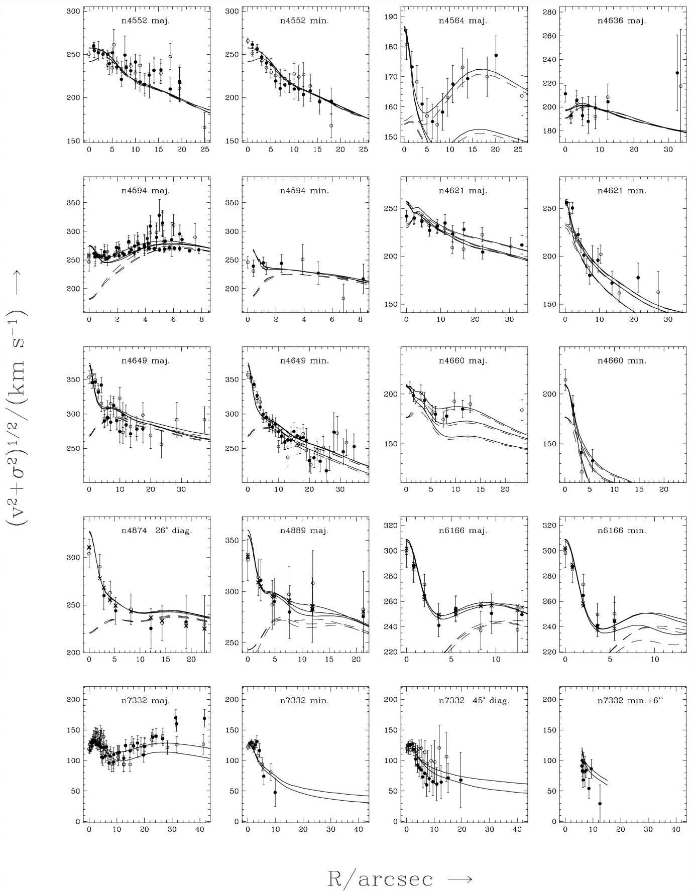
Figure 16.1: Velocity second moment \(\sqrt{V^2+\sigma^2}\) versus radius in the centers of selected massive galaxies (Magorrian et al. 1998). The solid curves are for the best-fit model with SMBH, the dashed curves for that without SMBH; different curves with the same linestyle are for different galaxy inclinations.
As we will discuss further below, Magorrian et al. (1998) used these measurements to determine the mass distribution of SMBHs for the first time.
The most general steady-state axisymmetric models depend on three integrals of motion as \(f(E,L_z,I_3)\). Because there is typically no analytic expression for \(I_3\), such models are most easily constructed using Schwarzschild modeling (Chapter 14.3). The practical implementation of Schwarzschild modeling follows the approach discussed in Chapter 14.3.3 and as usual consists of deprojecting the observed surface density to a luminosity profile, converting the luminosity to stellar mass using an assumed mass-to-light ratio, creating the full gravitational potential by adding an SMBH, integrating orbits in this potential, and optimizing their weights to fit the photometric and kinematic data. Aside from the ability to create three-integral models, an advantage of Schwarzschild modeling is that it can easily fit the full structure of the line-of-sight velocity distribution rather than just its second moment, either by representing it using Gauss-Hermite moments (Rix et al. 1997; Cretton et al. 1999) or fitting the full distribution (Gebhardt et al. 2003). Another late-1990s development was the ability to measure the line-of-sight kinematics on small angular scales with HST, allowing the central velocity structure to be much better resolved than was possible from the ground. These advances allowed high-significance detections of SMBHs in various galaxies (e.g., van der Marel et al. 1998; Cretton & van den Bosch 1999; Gebhardt et al. 2000b). Figure 16.2 shows some of the result of Schwarzschild modeling of the inner regions of 6 galaxies from Gebhardt et al. (2003); while the entire line-of-sight velocity distribution is included in the fit, for convenience the data and the model have been summarized as \(\sqrt{V^2+\sigma^2}\) versus radius in arcseconds.
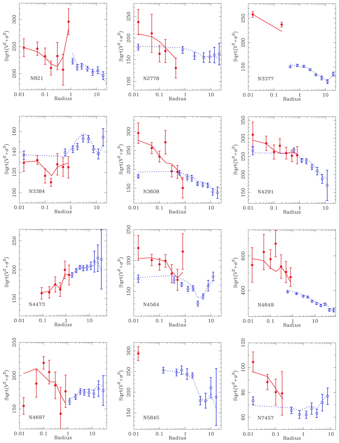
Figure 16.2: Velocity second moment \(\sqrt{V^2+\sigma^2}\) versus radius fit with Schwarzschild models (Gebhardt et al. 2003). The blue data points are ground-based data, while the red data have been obtained with HST. The curves are the best-fit model with SMBH, convolved with the ground-based and HST resolutions.
The HST data in red show that the velocity dispersion remains large or increases well within the sphere of influence for these galaxies, which when included in the full orbital modeling provides strong evidence for SMBHs. The Schwarzschild models also allow us to determine the importance of the third integral and, thus, whether the two-integral models discussed above are valid. Generally, Schwarzschild models demonstrate that the ratio \(\sigma_R/\sigma_z\) varies within each galaxy, but that the average value across galaxies is \(\sigma_R/\sigma_z \approx 1\) (Gebhardt et al. 2003). As a consequence, for an individual SMBH, two-integral models can be off by a factor of a few in \(M_\bullet\), but on the whole they obtain roughly the correct SMBH mass and mass distribution.
The two-integral and, later, three-integral models of dozens of SMBHs allowed their population statistics to be determined. Magorrian et al. (1998) used their large sample of SMBH masses to take a first look at the mass distribution, in particular, the distribution of the ratio \(x = M_\bullet/M_\mathrm{bulge}\). Various fits to this distribution are displayed Figure 16.3 from Magorrian et al. (1998).
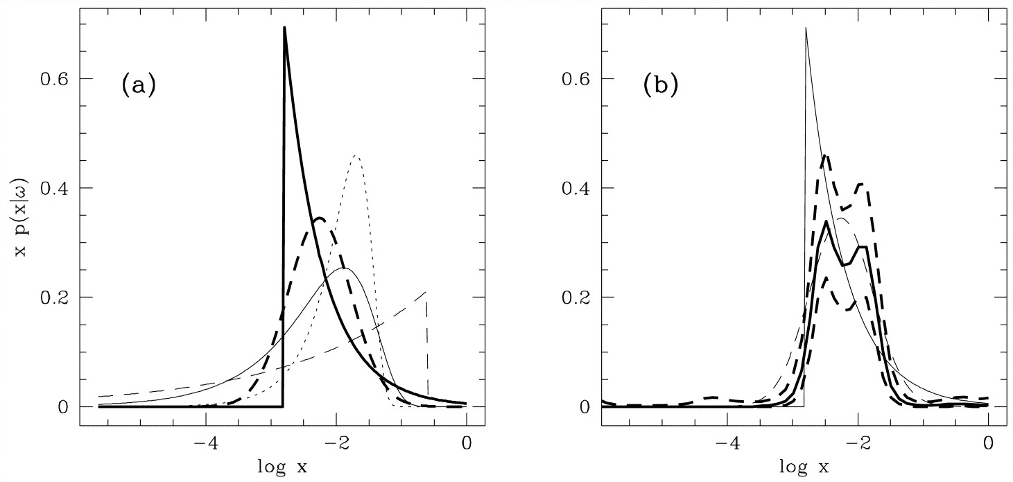
Figure 16.3: SMBH mass distribution as a function of \(x = M_\bullet/M_\mathrm{bulge}\) (Magorrian et al. 1998). The different curves in the left panel are different parametric models for the mass distribution, while the right panel shows a non-parametric reconstruction with uncertainty shown as the thick solid and dashed lines (one of the parametric models is repeated).
While the relatively small number of SMBH masses leaves some uncertainty in the exact mass distribution, both parametric and non-parametric reconstructions of the distribution of \(x\) agree that \(10^{-3} \lesssim M_\bullet/M_\mathrm{bulge} \lesssim 10^{-2}\) and SMBHs therefore are typically a few tenths of a percent of the mass of the bulge. As we saw above, this is enough to significantly change the orbital distribution within and just outside the sphere of influence, but it doesn’t directly affect the larger-scale orbital structure of the galaxy. However, the orbital distribution within the sphere of influence is correlated with the larger-scale structure of the elliptical galaxy that the SMBH lives in: The Schwarzschild models from Gebhardt et al. (2003) demonstrate that the orbits within the sphere of influence are tangentially biased for galaxies whose inner density profile is a shallow cusp (the so-called “core” galaxies discussed in Chapter 12.1) , while galaxies with a steeper inner-density cusp have kinematics that is more typically isotropic (see Chapter 13.4.2 for a discussion of the larger-scale orbital structure of these systems). Tangentially-biased orbits are consistent with the influence of a binary black hole (Faber et al. 1997) expected to form when an elliptical galaxy forms through a major merger of two smaller galaxies; as the second black hole sinks to the center, it preferentially scatters radial orbits out of the core (Nakano & Makino 1999). The more isotropic models are consistent with the black hole growing through quiescent, adiabatic growth (Quinlan et al. 1995). As we will see below, this is consistent with other lines of evidence regarding the origin of the two main classes of elliptical galaxies.
The distribution of \(M_\bullet/M_\mathrm{bulge}\) above shows that, while the SMBH constitutes only a small fraction of the mass of a galaxy, its mass is closely related to the mass of the galaxy it lives in. The relation between an SMBH and its galaxy host is the area of study known as black-hole–galaxy scaling relations. In their review of the eight SMBH detections known at the time, Kormendy & Richstone (1995) showed that \(M_\bullet\) is correlated with the luminosity of the bulge. This started a search for the galaxy property that is most tightly correlated to SMBH mass, culminating in the discovery of the M–sigma relation: the fact that among all galaxy properties, \(M_\bullet\) appears to be most strongly correlated with the velocity dispersion of the bulge (Ferrarese & Merritt 2000; Gebhardt et al. 2000a; for an elliptical galaxy, the “bulge” is the entire galaxy). This is illustrated well in Figure 16.4 from Gebhardt et al. (2000a), which shows the correlation of \(M_\bullet\) with bulge luminosity \(L_B\) on the one hand and bulge velocity dispersion \(\sigma_e\) on the other hand; it is clear that the velocity dispersion has much smaller scatter around the power-law model than the luminosity.
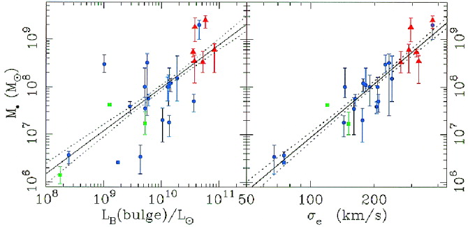
Figure 16.4: SMBH mass vs. bulge luminosity (left) and vs. bulge velocity dispersion (right; Gebhardt et al. 2000a).
The discovery of the tight relations between \(M_\bullet\) and the properties of the bulge created a rich field studying the co-evolution of SMBHs and their host galaxies (e.g., Silk & Rees 1998; Volonteri et al. 2003; Granato et al. 2004; Di Matteo et al. 2005; Croton et al. 2006; see Kormendy & Ho 2013 for a review). To better constrain the link between SMBHs and their host galaxy, much effort has been put into measuring the scaling relations between \(M_\bullet\) and \(\sigma_e\) or \(L_B\) better and into determining their intrinsic scatter (e.g., Tremaine et al. 2002). After two decades of work, it is clear that there is significant intrinsic scatter in the relation, at the level of \(0.3\,\mathrm{dex}\) in \(\log_{10} M_\bullet\), and that this intrinsic scatter is at least somewhat related to the type of galaxy (elliptical or spiral [e.g., Gültekin et al. 2009]; active or quiescent [e.g., Greene & Ho 2006]; shallow or steep inner density profile [e.g., McConnell & Ma 2013]). Because of these variations, the normalization and power-law slope of the relations depends on the sample used to measure them, but the relation found by Gültekin et al. (2009) is a reasonable typical relation \begin{equation}\label{eq-massellip-Msigma} M_\bullet = 1.3\times 10^8\,M_\odot\,\left({\sigma_e \over 200\,\mathrm{km\,s}^{-1}}\right)^{4.24}\,, \end{equation} with an uncertainty in the power-law of \(0.4\), an uncertainty in the normalization of \(\approx 20\%\), and an intrinsic scatter of \(\approx0.45\,\mathrm{dex}\) in \(\log_{10}M_\bullet\) when considering all galaxy types (\(\approx 0.30\,\mathrm{dex}\) when only considering elliptical galaxies). Similarly, other relations between \(M_\bullet\) and the mass of the bulge \(M_\mathrm{bulge}\) (\(M_\bullet \propto M_\mathrm{bulge}^{1.12}\); Marconi & Hunt 2003; Häring & Rix 2004) and even with the mass of the entire dark-matter halo \(M_\mathrm{halo}\) (Ferrarese 2002) have proven to be useful.
As we discussed above using Equation (16.4), measurements of the mass within the sphere of influence probe the central mass at about \(10^6\) times the SMBH’s Schwarzschild radius \(r_\bullet\) and even the high-resolution HST data do not come much closer than \(\approx 10^5\,r_\bullet\). Therefore, while the stellar kinematics measurements can establish the presence of a dense concentration of mass, they cannot unambiguously show that this concentration is in fact a black hole. So why do we believe that the central-mass concentrations in massive galaxies are black holes? All arguments for this are indirect. One argument, which was important for getting the search for SMBHs started, is that the active galactic nuclei and quasars seen at higher redshift are most easily explained as resulting from the accretion of gas onto massive black holes (e.g., Salpeter 1964; Zel'dovich 1964; Lynden-Bell 1969; Rees 1984) and evidence for the black-hole paradigm comes from such observations as the rapid variability in the quasar light and superluminal jets (Rees 1966). Quasars were much more common at redshifts \(\gtrsim 2\) than they are in the present-day Universe and if they are powered by accretion onto a black hole, quiescent SMBHs should hide within massive galaxies today (Lynden-Bell 1969). A simple argument by Soltan (1982) (known as the Soltan argument) allows one to connect the total luminosity density of quasars at high redshift to the mass density of SMBHs today, simply by assuming that the quasar luminosity results from accretion through \(L = \varepsilon \dot{M}c^2\), where \(\varepsilon\) describes the efficiency of the accretion (which has to be \(\sim 10\%\) explain quasars, much higher than the efficiency achievable through, e.g., nuclear burning). The mass density of \(\approx 2\times 10^5\,M_\odot\,\mathrm{Mpc}^{-3}\) that one obtains from this argument (Chokshi & Turner 1992) combined with the density of massive galaxies then shows that each massive galaxy should host an SMBH with \(\approx 10^8\,M_\odot\). The consistency of this number with the observed SMBH masses and their spatial density (Merritt & Ferrarese 2001) demonstrates that SMBHs are likely the quiescent black-hole remnants of high-redshift quasars.
A further indirect argument comes from those systems where we can measure the central mass much closer to the Schwarzschild radius. Galaxies with detected nuclear masers allow the central mass to be constrained to \(r \lesssim 0.1\,\mathrm{pc}\), where the implied density is much higher. For example, the maser detection of the SMBH in NGC 4258 constrains the central mass to be \(3.6\times 10^7\,M_\odot\) within \(0.13\,\mathrm{pc}\) (Miyoshi et al. 1995); this density is so high that there is no other known stable physical system of such high density. But the best dynamical evidence for an SMBH is found in the Milky Way, where the star S2 is observed to have a Keplerian orbit with a pericenter of only \(\approx 6\times10^{-4}\,\mathrm{pc} = 120\,\mathrm{AU} \approx 1,400\,r_\bullet\) (Schödel et al. 2002; Ghez et al. 2003). Detailed measurements of S2’s orbit (and that of other, similar stars) measure the Milky Way’s SMBH to be \(M_\bullet \approx 4.3\times 10^6\,M_\odot\) (Ghez et al. 2008; Gillessen et al. 2009). The implied density is so high that it is difficult to imagine any other physical object than a black hole. Recent high-resolution interferometric observations have furthermore allowed the relativistic effects of the gravitational redshift (Gravity Collaboration et al. 2018; Do et al. 2019) and the pericenter precession (Gravity Collaboration et al. 2020) to be detected at high significance. There is thus little doubt now that the central object in the Milky Way is a black hole.
Definitive proof that the population of what we have referred to as SMBHs is in fact a population of black holes will likely have to wait until space-based interferometers like LISA are able to detect the gravitational wave signature of the inspiral and merger of binary SMBHs.

 .
. .
. .
.