
14.2. Are elliptical galaxies flattened by rotation?
Now that we have derived the tensor-virial theorem and now that we understand the potential-energy tensor of oblate spheroids, we can use the tensor-virial theorem to understand the basic dynamical structure of elliptical galaxies. We will focus here on axisymmetric elliptical galaxies and ask the question “Is the oblateness of such elliptical galaxies caused by rotation?”. What we mean more specifically with this question is the following. Observations of elliptical galaxies demonstrate that the velocity dispersion of stars is much larger than that of stars in disk galaxies. Unlike for disk galaxies, the dynamical support against gravitational collapse for elliptical galaxies therefore comes from their velocity dispersion rather than ordered rotation and we say that elliptical galaxies are pressure-supported systems. However, a non-rotating system with an isotropic velocity-dispersion tensor has to be spherical, as is clear from the tensor virial theorem with \(\vec{T}_{\alpha\beta} = 0\) (for zero rotation): \begin{equation} \vec{\Pi}_{\alpha\beta} = -\vec{W}_{\alpha\beta}\,; \end{equation} If \(\vec{\Pi}_{\alpha\beta} = M\,\sigma^2\,\delta^{\alpha\beta}\) then \(\vec{W}_{\alpha\beta} \propto \delta^{\alpha\beta}\) as well and this is only the case for a spherical system (see the argument following Equation 14.35). There are, therefore, two ways in which a gravitational system can be flattened: (i) through rotation, such that \(\vec{T}_{\alpha\beta} \neq 0 \neq \delta^{\alpha\beta}\), or (ii) through an anisotropic velocity dispersion tensor. The question “Are elliptical galaxies flattened by rotation?” therefore specifically asks whether elliptical galaxies can be flattened by rotation alone, that is, by having the galaxy rotate while keeping the velocity dispersion isotropic.
Let’s therefore consider a model for an elliptical galaxy that is a flattened spheroid with an axis ratio \(q\) and that has an overall rotation around the \(z\) axis with a velocity \(v\) and isotropic velocity dispersion \(\sigma\). For this model, \begin{align} \vec{T}_{\alpha\beta} & = \frac{M\,v^2}{4}\,\delta^{\alpha\beta}\,(1-\delta^{\alpha z})\,, \end{align} that is, only the \(xx\) and \(yy\) diagonal elements are non-zero and the total kinetic energy in rotation is \(T_{xx}+T_{yy}=Mv^2/2\). We also have \begin{align} \vec{\Pi}_{\alpha\beta} & = M\,\sigma^2\,\delta^{\alpha\beta}\,. \end{align} The tensor-virial theorem then states that \begin{equation} {M\,v^2\over 2}\,\delta^{\alpha\beta}\,(1-\delta^{\alpha z})+M\,\sigma^2\,\delta^{\alpha\beta}=-\vec{W}_{\alpha\beta}\,. \end{equation} If we then take the ratio of the \(xx\) and \(zz\) components of this equation and re-arrange the resulting expression, we obtain \begin{equation}\label{eq-tensorvirial-vsigmaellip-WxxWzz} \frac{v}{\sigma}= \sqrt{2\left(\frac{W_{xx}}{W_{zz}}-1\right)}\,. \end{equation} This equation makes sense in that for a spherical system, \(W_{xx}/W_{zz} = 1\), so \(v/\sigma = 0\) corresponding to the fact that a spherical, isotropic system does not rotate. For a flattened system, \(W_{xx}/W_{zz} > 1\), so \(v/\sigma > 0\).
For an oblate spheroid, we know that the ratio \(W_{xx}/W_{zz}\) only depends on the axis ratio \(q\) (Equation 14.38), so we have that \begin{equation}\label{eq-tensorvirial-vsigmaellip-F} \frac{v}{\sigma}= \sqrt{2\left[F(q)-1\right]}\,, \end{equation} where \(F(q) = W_{xx}/W_{zz}\) is the inverse of Equation (14.38), or explicitly (using the eccentricity \(e = \sqrt{1-q^2}\) instead of \(q\)) \begin{equation}\label{eq-tensorvirial-vsigmaellip-full} \frac{v}{\sigma}= \sqrt{\frac{1}{(1-e^2)}\,\frac{\left(\frac{\sin^{-1}e}{e}-\sqrt{1-e^2}\right)}{\left(\frac{1}{\sqrt{1-e^2}}-\frac{\sin^{-1} e}{e}\right)}-2}\,, \end{equation} This function is shown in Figure 14.3.
[11]:
# To better resolve the behavior near e=1, use a denser grid there
e_vsigma= numpy.hstack((numpy.linspace(1e-4,0.5,51),
                     sorted(1.-numpy.geomspace(1e-4,0.5,51))))
figure(figsize=(6,4))
#Wzz_over_Wxx(.) and q_from_e defined in the previous section
def Wzz_over_Wxx(e):
    return 2.*(1.-e**2.)*(1./numpy.sqrt(1.-e**2.)-numpy.arcsin(e)/e)/(numpy.arcsin(e)/e-numpy.sqrt(1.-e**2.))
def q_from_e(e):
    return numpy.sqrt(1.-e**2.)
plot(e_vsigma,numpy.sqrt(2./Wzz_over_Wxx(e_vsigma)-2.),
     label=r'$\mathrm{Exact}$')
plot(e_vsigma,4./numpy.pi*numpy.sqrt((1-q_from_e(e_vsigma))/q_from_e(e_vsigma)),
    label=r'$(4/\pi)\mathrm{\sqrt{\varepsilon/(1-\varepsilon)}\ approximation}$')
xlabel(r'$e$')
ylabel(r'$v/\sigma$')
ylim(0.,3.)
legend(frameon=False,fontsize=18.);

Figure 14.3: Ratio of the rotation velocity \(v\) to the velocity dispersion \(\sigma\) for a flattened isotropic rotator, including a simple approximate form for the relation.
Remarkably, to an accuracy of about one percent over the entire range of axis ratios, this function can also be approximated as (Kormendy 1982) \begin{equation}\label{eq-tensorvirial-vsigmaellip-ellipticity} \frac{v}{\sigma} \approx {4\over \pi}\,\sqrt{\frac{1-q}{q}}={4\over \pi}\,\sqrt{\frac{\varepsilon}{1-\varepsilon}}\,, \end{equation} where the ellipticity \(\varepsilon = 1-q\) (not to be confused with the eccentricity). Comparing this approximation to the full expression from Equation (14.45), we see that they agree very well in Figure 14.3.
Equation (14.45) cannot be directly used to compare to observations for a few reasons. The first is that most galaxies are not seen edge-on, but are inclined. The effect of the inclination is to reduce the observed velocity while keeping the (isotropic) velocity dispersion the same. We therefore have that \(\left({v/\sigma}\right)_\mathrm{obs} = \left({v / \sigma}\right)\,\sin i\). Averaging over random inclinations, we have that \(\langle \sin i \rangle = \pi/4\) (Binney 1978b), which implies that on average we expect \begin{equation}\label{eq-tensorvirial-vsigmaobs-2} \left\langle{v \over \sigma}\right\rangle_\mathrm{obs}= {\pi \over 4}\sqrt{2\left[F(q)-1\right]} \approx \sqrt{\frac{\varepsilon}{1-\varepsilon}}\,. \end{equation} where we used Equation (14.46) for the final, again remarkable, approximation.
The second observational complication is how we actually measure the ‘\(v\)’ and ‘\(\sigma\)’ that appear in these expressions. They represent global averages defined through the ordered and random part of the kinetic energy tensor, but traditionally they are estimated by the peak of the rotation velocity and the centrally-averaged velocity dispersion. Equation (14.47) with these estimates is how this formalism was applied until the advent of integral-field-spectroscopy surveys (IFS) in the mid-2000s (see Chapter 16.2 and following for a detailed discussion of these). IFS observations, however, allow the mean velocity and velocity dispersion to be determined over a wide, two-dimensional area of the galaxy. This allows for a more rigorous application of the tensor-virial-theorem formalism. In particular, Binney (2005) showed that when defining ‘\(v\)’ and ‘\(\sigma\)’ as the luminosity-weighted mean line-of-sight velocity and velocity dispersion, the predicted observed value of \(v/\sigma\) for a galaxy with inclination \(i\) becomes approximately \begin{equation}\label{eq-tensorvirial-vlossigmalos} \left({v \over \sigma}\right)_\mathrm{obs}= \sqrt{\frac{F(q)-1}{0.15\,F(q)+1}}\,\sin i\,, \end{equation} in terms of \(F(q) = W_{xx}/W_{zz}\) introduced in Equation (14.44), where the \(0.15\) factor is set by the shape of the luminosity profile (Cappellari et al. 2007). Another complication is that we can only determine the observed, projected ellipticity, not the intrinsic ellipticity that goes in Equation (14.46) and the ratio of intrinsic-to-observed ellipticity is typically \(\approx 2\) (Weijmans et al. 2014), although because inclinations are random, it of course has a wide variation. When plotting \(v/\sigma\) versus ellipticity, both are affected by the inclination and its effect is therefore complex. The relation between the intrinsic ellipticity \(\varepsilon\) and the projected (observed) ellipticity \(\varepsilon_{\mathrm{obs}}\) is \begin{equation} \varepsilon = 1-\sqrt{1+\varepsilon_{\mathrm{obs}}(\varepsilon_{\mathrm{obs}}-2)/\sin^2 i}\,. \end{equation} We then plot the predicted observed \(v/\sigma\) for an isotropic rotator as a function of observed ellipticity for a few values of the inclination in Figure 14.4 (only considering galaxies with intrinsic ellipticities \(<0.8\)).
[12]:
def eps_intrin(eps_obs,sini):
    return 1.-numpy.sqrt(1.+eps_obs*(eps_obs-2.)/sini**2.)
# Relation between intrinsic e and q from previous section
def e_from_q(q):
    return numpy.sqrt(1.-q**2.)
def vsigma_observed_ellipticity(eps_obs,sini=1):
    """Return v/sigma for a given observed ellipticity
    eps and sine(inclination)"""
    eps= eps_intrin(eps_obs,sini)
    # Don't deal with e_intrin > 0.8
    eps[eps>0.8]= numpy.nan
    e_intrin= e_from_q(1.-eps)
    out= numpy.sqrt((1./Wzz_over_Wxx(e_intrin)-1.)/(0.15/Wzz_over_Wxx(e_intrin)+1.))
    return out*sini
eps_obs= numpy.linspace(1e-4,1-1e-4,101)
figure(figsize=(6,4))
plot(eps_obs,vsigma_observed_ellipticity(eps_obs,sini=1.),
     label=r'$\sin i = 1$')
plot(eps_obs,vsigma_observed_ellipticity(eps_obs,sini=numpy.pi/4.),
     label=r'$\sin i = \pi/4$')
plot(eps_obs,vsigma_observed_ellipticity(eps_obs,sini=0.6),
     label=r'$\sin i = 0.6$')
xlabel(r'$\varepsilon_\mathrm{obs}$')
ylabel(r'$\left(v/\sigma\right)_\mathrm{obs}$')
ylim(0.,1.4)
legend(frameon=False,fontsize=18.);

Figure 14.4: Observed ratio of the rotation velocity \(v\) to the velocity dispersion \(\sigma\) for a flattened isotropic rotator for different inclinations.
As expected, going from an edge-on to a face-on configuration increases the required \(v/\sigma\), because the intrinsic ellipticity is higher than the observed one for more face-on systems and this higher ellipticity requires higher \(v/\sigma\) to be supported. If elliptical galaxies are oblate, isotropic rotators, they should therefore lie above the lowest line, with their exact predicted location depending on their inclinations.
We can compare these predictions to observations of \(v/\sigma\) and ellipticity for many elliptical galaxies, for example, the sample of galaxies from the integral-field surveys ATLAS\(^\mathrm{3D}\) and SAMI shown in Figure 14.5.
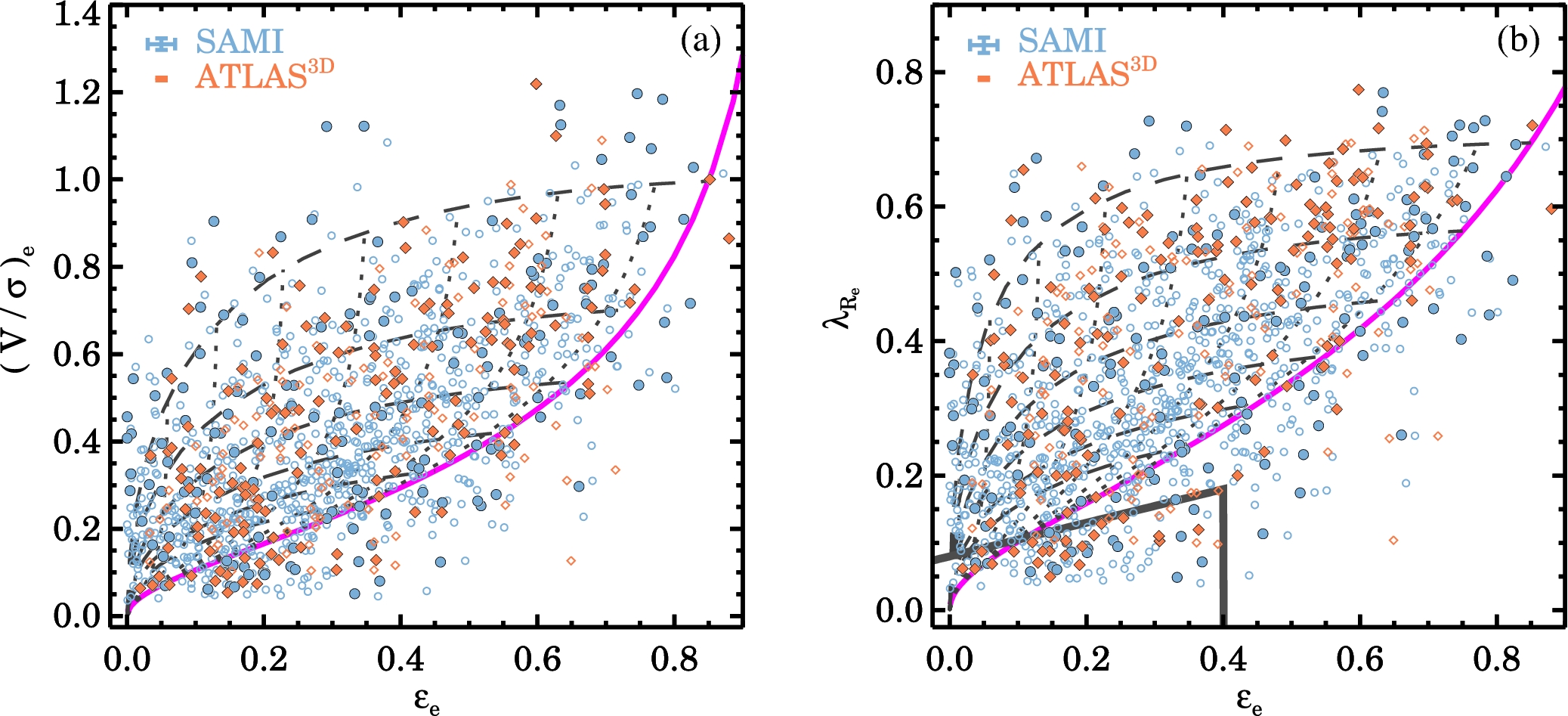
Figure 14.5: Observed ratio of the rotation velocity \(v\) to the velocity dispersion \(\sigma\) for elliptical galaxies from the SAMI and ATLAS\(^{\mathrm{3D}}\) surveys (van de Sande et al. 2017).
By comparing these observations to the curves in the previous figure, we see that many of the observed galaxies lie below the edge-on isotropic-rotator curve and almost all galaxies lie below the \(\sin i = \pi/4\) curve, which is the average inclination. Thus, most elliptical galaxies cannot be fully-isotropic rotators and anisotropy in the velocity dispersion must play a big role in the dynamical support of elliptical galaxies.

 .
. .
. .
.