
8.3. The kinematics of the Milky Way’s interstellar medium
8.3.1. The longitude-velocity diagram
In the Milky Way, we can also observe the kinematics of tracers such as HI and CO to study galactic rotation. A complication, however, is that the observer’s (i.e., our own) position is itself participating in the rotation of the disk and the observed velocities of the gas therefore reflect both intrinsic galactic rotation as well as the motion of the Sun and Earth. This greatly complicates measuring the rotation curve of the Milky Way from the kinematics of the interstellar medium (or from the kinematics of any disk tracer really). Despite this complication, the kinematics of the interstellar medium contains a wealth of information about the rotation of the Milky Way and perturbations to circular rotation from the influence of, e.g., the bar and spiral structure. In this section, we will only consider motions in the mid-plane of the Milky Way and ignore the motion perpendicular to the mid-plane, because we may assume that gas orbits in the mid-plane (at least at \(R \lesssim 10\,\mathrm{kpc}\)).
We will work in the following approximation. No matter whether the gas is on circular or closed orbits, we can assume that at a given position in the plane, gas can only have a single velocity. If this were not the case, gas trajectories would cross. At a point of crossing, non-gravitational forces would be important and significantly change the orbits, pushing them toward a single velocity. This is a powerful assumption, because it means that only a two-dimensional subspace of the four-dimensional phase-space of positions and velocities in the mid-plane is occupied by gas (because velocity space reduces to a single point at every \(\vec{x}\)). We can thus hope to observe the full phase-space distribution of gas from a two-dimensional projection of its phase-space onto observable quantities.
Just like in external galaxies, we can observe the intensity of emission from the interstellar medium at different wavelengths at any sky position in the mid-plane by obtaining a spectrum at this position. This spectrum can be converted to a distribution of emission as a function of velocity \(v_\mathrm{los}\) by interpreting wavelength shifts from the restframe wavelength of, say, the HI 21cm line, as Doppler velocity shifts. By going around the Milky Way as a function of Galactic longitude \(l\), we can therefore map the intensity of emission as a function of \((l,v_\mathrm{los})\). Thus, we obtain the so-called longitude–velocity diagrams of different tracers of the interstellar medium. One of the main ones of interest of these is the HI 21cm emission shown in Figure 8.13.

Figure 8.13: Longitude-velocity diagram of neutral gas in the Milky Way. Created using data from the HI4PI survey (HI4PI Collaboration et al. 2016).
Another one is the \((l,v_\mathrm{los})\) diagram of molecular gas, for which we can use the molecular-cloud catalog of Miville-Deschênes et al. (2017). Because we will use the molecular-gas \((l,v_\mathrm{los})\) diagram to compare to models below, we first implement some functions to (a) download the data from Vizier, (b) read the GMC catalog, and (c) plot the \((l,v)\) distribution of the GMCs. To download the data from Vizier, we use the function that we defined in Section 8.2.2 to download a catalog from the Vizier service:
[9]:
# vizier.py: download catalogs from Vizier
import sys
from pathlib import Path
import shutil
import tempfile
from ftplib import FTP
import subprocess
_ERASESTR= "                                                                                "
def vizier(cat,filePath,ReadMePath,
           catalogname='catalog.dat',readmename='ReadMe'):
    """
    NAME:
       vizier
    PURPOSE:
       download a catalog and its associated ReadMe from Vizier
    INPUT:
       cat - name of the catalog (e.g., 'III/272' for RAVE, or J/A+A/... for journal-specific catalogs)
       filePath - path of the file where you want to store the catalog (note: you need to keep the name of the file the same as the catalogname to be able to read the file with astropy.io.ascii)
       ReadMePath - path of the file where you want to store the ReadMe file
       catalogname= (catalog.dat) name of the catalog on the Vizier server
       readmename= (ReadMe) name of the ReadMe file on the Vizier server
    OUTPUT:
       (nothing, just downloads)
    HISTORY:
       2016-09-12 - Written as part of gaia_tools - Bovy (UofT)
       2017-09-12 - Copied to galdyncourse (yes, same day!) - Bovy (UofT)
       2019-12-20 - Copied directly into notes to avoid additional dependency - Bovy (UofT)
    """
    _download_file_vizier(cat,filePath,catalogname=catalogname)
    _download_file_vizier(cat,ReadMePath,catalogname=readmename)
    catfilename= Path(catalogname).name
    with open(ReadMePath,'r') as readmefile:
        fullreadme= ''.join(readmefile.readlines())
        if catfilename.endswith('.gz') and not catfilename in fullreadme:
            # Need to gunzip the catalog
            try:
                subprocess.check_call(['gunzip',filePath])
            except subprocess.CalledProcessError as e:
                print("Could not unzip catalog %s" % filePath)
                raise
    return None

def _download_file_vizier(cat,filePath,catalogname='catalog.dat'):
    sys.stdout.write('\r'+"Downloading file %s from Vizier ...\r" \
                         % (Path(filePath).name))
    sys.stdout.flush()
    try:
        # make all intermediate directories
        os.makedirs(Path(filePath).parent)
    except OSError: pass
    # Safe way of downloading
    downloading= True
    interrupted= False
    file, tmp_savefilename= tempfile.mkstemp()
    os.close(file) #Easier this way
    ntries= 1
    while downloading:
        try:
            ftp= FTP('cdsarc.u-strasbg.fr')
            ftp.login()
            ftp.cwd(str(Path('pub') / 'cats' / cat))
            with open(tmp_savefilename,'wb') as savefile:
                ftp.retrbinary('RETR %s' % catalogname,savefile.write)
            shutil.move(tmp_savefilename,filePath)
            downloading= False
            if interrupted:
                raise KeyboardInterrupt
        except:
            if not downloading: #Assume KeyboardInterrupt
                raise
            elif ntries > 5:
                raise IOError('File %s does not appear to exist on the server ...' % (Path(filePath).name))
        finally:
            if Path(tmp_savefilename).exists():
                os.remove(tmp_savefilename)
        ntries+= 1
    sys.stdout.write('\r'+_ERASESTR+'\r')
    sys.stdout.flush()
    return None
Then we read the catalog using astropy and convert it to a convenient pandas format:
[5]:
import os
from pathlib import Path
from astropy.io import ascii
_CACHE_BASEDIR= Path(os.getenv('HOME')) / '.galaxiesbook' / 'cache'
_CACHE_VIZIER_DIR= _CACHE_BASEDIR / 'vizier'
_MIVILLE_VIZIER_NAME= 'J/ApJ/834/57'
def gmc_read(verbose=False):
    """
    NAME:
       gmc_read
    PURPOSE:
       read the Miville-Deschênes GMC catalog
    INPUT:
       verbose= (False) if True, be verbose
    OUTPUT:
       pandas dataframe
    HISTORY:
       2017-09-12 - Written - Bovy (UofT)
    """
    # Generate file path and name
    tPath= _CACHE_VIZIER_DIR / 'cats'
    for directory in _MIVILLE_VIZIER_NAME.split('/'):
        tPath = tPath / directory
    filePath= tPath / 'table1.dat.gz'
    readmePath= tPath / 'ReadMe'
    # download the file
    if not Path(str(filePath)[:-3]).exists():
        vizier(_MIVILLE_VIZIER_NAME,filePath,readmePath,
               catalogname='table1.dat.gz',readmename='ReadMe')
    # Read with astropy, w/o the .gz
    table= ascii.read(str(filePath)[:-3],readme=str(readmePath),format='cds')
    return table.to_pandas()
Next we write a function to plot the \((l,v)\) diagram, because we will re-use it below:
[6]:
def gmc_plot_lv(**kwargs):
    data= gmc_read()
    data= data[numpy.fabs(data['GLAT']) < 2.]
    s= data['Area']*15.
    s[s>30.]= 30.
    c= 'k'
    out= scatter(data['GLON'],data['Vcent'],s=s,c=c,
                 cmap='gist_yarg',alpha=0.1,**kwargs)
    xlabel(r'$\mathrm{Galactic\ longitude}\,(\mathrm{deg})$')
    ylabel(r'$v_{\mathrm{los}}\,(\mathrm{km\,s}^{-1})$')
    xlim(185.,-185.)
    ylim(-200.,200.)
    return out
and then we plot the molecular-gas \((l,v_\mathrm{los})\) diagram:
[7]:
figure(figsize=(10,5),dpi=300)
data= gmc_plot_lv(rasterized=True)

Figure 8.14: Longitude-velocity diagram of molecular gas in the Milky Way.
Both the HI and the molecular-gas \((l,v_\mathrm{los})\) diagrams display a similar pattern, with a similar envelope tracing the edges of the distribution and similar features near \(l=0^\circ\), but the intensity is different at different locations because the density distribution of neutral hydrogen and molecular gas is different (see Chapter 1.2.2).
These \((l,v_\mathrm{los})\) diagrams are thus full representations of the phase-space distribution of the interstellar medium. In the remainder of this section, we will discuss the mapping of the four-dimensional phase-space distribution \(f(R,\phi,v_R,v_\phi)\) (in polar coordinates) onto \((l,v_\mathrm{los})\). A minor complication that we will see is that at some locations in the \((l,v_\mathrm{los})\) diagram, two different \((R,\phi,v_R,v_\phi)\) get projected onto the same \((l,v_\mathrm{los})\), so we can only recover \(f(R,\phi,v_R,v_\phi)\) up to this degeneracy.
8.3.2. Circular rotation and the longitude-velocity diagram
We start by determining the patterns in the \((l,v_\mathrm{los})\) [which we will abbreviate as \((l,v)\) from hereon] diagram that we would see for a disk of gas in circular rotation with a rotation curve \(v_c(R)\). As usual, we will work in a left-handed Milky-Way frame where the disk rotates clockwise when seen from the North Galactic Pole. For a parcel of gas at a position \(\vec{x}\) with respect to the Galactic center that is on a circular orbit at radius \(R = |\vec{x}|\), the velocity is \begin{equation} \vec{v} = \vec{v}_c(R)\times\vec{\hat{x}}\,, \end{equation} where \(\vec{v}_c(R)\) is a vector with magnitude \(v_c(R)\) that is perpendicular to the mid-plane (pointing towards negative \(z\), so we can work out cross products with the usual right-hand rule) and \(\vec{\hat{x}}\) is the unit vector in the direction of \(\vec{x}\). We will assume that the observer itself is on a circular orbit at position \(\vec{x}_0\) with radius \(R_0=|\vec{x}_0|\) and velocity \(\vec{v}_0 = \vec{v}_c(R_0)\times\vec{\hat{x}}_0\); this orbit is called the local standard of rest (LSR) and we can approximately correct the Sun’s peculiar motion with respect to the LSR (which is about \(10\,\mathrm{km\,s}^{-1}\), although the exact value is still under debate; see Chapter 10.3.1). The observed line-of-sight velocity \(v_\mathrm{los}\) is then the projection of the velocity difference \((\vec{v}-\vec{v}_0)\) onto the line-of-sight direction \((\vec{x}-\vec{x}_0)/|\vec{x}-\vec{x}_0|\) \begin{align} v_\mathrm{los} & = (\vec{v}-\vec{v}_0)\cdot\frac{\vec{x}-\vec{x}_0}{|\vec{x}-\vec{x}_0|}= \left(\vec{v}_c(R)\times\vec{\hat{x}}-\vec{v}_c(R_0)\times\vec{\hat{x}}_0\right)\cdot\frac{\vec{x}-\vec{x}_0}{|\vec{x}-\vec{x}_0|}\,. \end{align} We can work this out further by expanding the dot product, writing \(\vec{v}_c(R) = \vec{\Omega}(R)\,R\), and using that \(\vec{a}\cdot(\vec{a}\times\vec{b}) = 0\) and \(\vec{a}\cdot(\vec{b}\times\vec{c}) = \vec{b}\cdot(\vec{c}\times\vec{a})\). We end up with \begin{align} v_\mathrm{los} & = \left[\vec{\Omega}(R)-\vec{\Omega}(R_0)\right]\cdot\frac{\left(\vec{x}_0\times\vec{x}\right)}{|\vec{x}-\vec{x}_0|}\,. \end{align} Using basic geometry, the last factor is equal to \(-R_0\,\sin l\,\vec{\hat{n}}\), where \(\vec{\hat{n}}\) is the unit vector perpendicular to the mid-plane pointing toward the North Galactic Pole. The rotation vector \(\vec{\Omega} = -|\vec{\Omega}|\,\vec{\hat{n}}\) and thus we get the final result \begin{align}\label{eq-vlos-midplane-omega} v_\mathrm{los}(l) & = \left[\Omega(R)-\Omega(R_0)\right]\,R_0\,\sin l\,. \end{align} This equation makes sense for the following reasons: (i) a disk in solid-body rotation has \(\Omega(R) = \mathrm{constant}\) and therefore \(v_\mathrm{los} = 0\) from Equation (8.23); this must be the case because in a disk in solid-body rotation, the distance between any two points remains constant and there can, therefore, be no non-zero line-of-sight velocities. Also, (ii) at \(l=0\) and \(l=180^\circ\), the line-of-sight velocity coincides with (minus) the Galactocentric radial velocity, which is zero for a disk in circular rotation; Equation (8.23) indeed gives \(v_\mathrm{los} = 0\) at \(l=0\) and \(l=180^\circ\). Finally, (iii) it is clear that the expression of \(v_\mathrm{los}(l)\) needs to involve the subtraction of the projection of the LSR motion onto the line of sight, which is \(-v_c(R_0)\,\sin l = -\Omega(R_0)\,R_0\,\sin l\); therefore \(R_0\sin l\) must multiply \(\left[\Omega(R)-\Omega(R_0)\right]\).
Let’s now explore how gas at different \((R,\phi)\) gets mapped onto the \((l,v)\) plane using Equation (8.23) as our guide. Gas on a circular ring at radius \(R_c\) has a constant \(\Omega(R_c)\) along the ring. Equation (8.23) therefore tells us that this ring will map onto a sinusoidal curve \(\propto \sin l\) with prefactor \(\left[\Omega(R_c)-\Omega(R_0)\right]R_0\). For \(R_c < R_0\), the ring does not subtend the entire longitude range, but runs from \(-\mathrm{arcsin}(R_c/R_0)\) to \(\mathrm{arcsin}(R_c/R_0)\). At \(R_c > R_0\), the ring subtends the entire range of Galactic longitudes.
If we then assume a rotation curve \(v_c(R)\), we can map any ring at \(R_c\) to a locus in the \((l,v)\) plane. In Figure 8.15, we do this for rings at a few different radii assuming a flat rotation curve (using galpy’s LogarithmicHaloPotential) and overlaying the locations of the rings on the map of the molecular clouds from Miville-Deschênes et al. (2017), using the function to plot this data that we defined above.
[8]:
from galpy import potential
# Function to map (l,R) -> vlos
def vlos_ring(ls,Rc,pot=None,ro=8.):
    return (pot.omegac(Rc)-pot.omegac(ro))*ro*numpy.sin(ls)
figure(figsize=(10,5),dpi=300)
# First plot the GMCs
data= gmc_plot_lv(rasterized=True)
ro= 8.*u.kpc
vo= 220.*u.km/u.s
lp= potential.LogarithmicHaloPotential(normalize=1.,
                                       vo=vo,ro=ro)
Rc= 3.*u.kpc
ls= numpy.linspace(-numpy.arcsin(Rc/ro),numpy.arcsin(Rc/ro),101)
line_3= plot(ls.to(u.deg),vlos_ring(ls,Rc,pot=lp,ro=ro).to(u.km/u.s),lw=3.,
            label=r'$R = %.0f\,\mathrm{kpc}$' % Rc.to(u.kpc).value)
Rc= 6.*u.kpc
ls= numpy.linspace(-numpy.arcsin(Rc/ro),numpy.arcsin(Rc/ro),101)
line_6= plot(ls.to(u.deg),vlos_ring(ls,Rc,pot=lp,ro=ro).to(u.km/u.s),lw=3.,
            label=r'$R = %.0f\,\mathrm{kpc}$' % Rc.to(u.kpc).value)
Rc= 12.*u.kpc
ls= numpy.linspace(-numpy.pi,numpy.pi,101)*u.rad
line_12= plot(ls.to(u.deg),vlos_ring(ls,Rc,pot=lp,ro=ro).to(u.km/u.s),lw=3.,
             label=r'$R = %.0f\,\mathrm{kpc}$' % Rc.to(u.kpc).value)
Rc= 20.*u.kpc
ls= numpy.linspace(-numpy.pi,numpy.pi,101)*u.rad
line_20= plot(ls.to(u.deg),vlos_ring(ls,Rc,pot=lp,ro=ro).to(u.km/u.s),lw=3.,
             label=r'$R = %.0f\,\mathrm{kpc}$' % Rc.to(u.kpc).value)
legend(handles=[line_3[0],line_6[0],
               line_12[0],line_20[0]],
       fontsize=18.,loc='upper left',frameon=False);

Figure 8.15: Location of circularly-rotating rings in the longitude-velocity diagram from Figure 8.14.
We see that the features which run from the top-left center of this figure to the bottom-right center arise from rings inside of the solar circle, \(R_c < R_0\). The material at negative \(v_\mathrm{los}\) for \(l >0\) (left side) and positive \(v_\mathrm{los}\) for \(l < 0\) (right side) comes from rings outside of the solar circle. Very few clouds are found outside of the red curve for \(R_c = 20\,\mathrm{kpc}\), indicating that very little molecular gas is located that far from the center.
The molecular-gas distribution in Figure 8.14 has a strong overdensity that runs from the top-left center to the bottom-right center. It should now be clear that this is naturally explained if much molecular gas is found in a ring, somewhere between the blue and orange curves in Figure 8.15. A ring of \(R_c \approx 4.5\,\mathrm{kpc}\) provides a good match to the overdense feature (at least at positive \(l\)), indicating that there is an overdensity of molecular gas around \(R \approx 4.5\,\mathrm{kpc}\) in the Milky Way.
Coming back to galactic rotation, we can learn a few things from Equation (8.23). One is that the observed \(v_\mathrm{los}\) is only sensitive to \(\Omega(R)-\Omega(R_0)\), that is, differences in angular rotation rate. Adding a constant rotation rate \(\Omega_\mathrm{add}\) therefore does not change anything about the observed \((l,v)\) distribution. However, if we assume that as \(R \rightarrow \infty\) that \(\Omega(R) \rightarrow 0\), then Equation (8.23) tells us that \(v_\mathrm{los}(l) = -\Omega(R_0)\,R_0\,\sin l = -v_c(R_0)\,\sin l\) as \(R \rightarrow \infty\) and rings would bunch up near this “final” curve as we go to larger \(R\). Therefore, if we could measure the location of this final curve by delineating the outermost contour in the \((l,v)\) diagram, we could measure the circular velocity at the Sun’s location. The problem with this measurement is that it is difficult to see gas at large enough \(R\) for the limit \(R \rightarrow \infty\) to well describe the rotation curve. For example, for a flat rotation curve we have that \(\Omega(R) \propto \Omega(R_0)\,R_0/R\) and therefore for \(\Omega(R)\) to be, e.g., only 10% of \(\Omega(R_0)\), we require \(R = 10\,R_0 \approx 80\,\mathrm{kpc}\), where there is essentially no gas in the disk.
Therefore, to do this type of measurement of \(v_c(R_0)\) in the Milky Way, we require a model for the surface-density distribution \(\Sigma_{HI}(R)\) of the neutral hydrogen (we use neutral hydrogen, because CO has a shorter scale length than HI) and we can then predict the amount of HI as a function of \(v_\mathrm{los}\) by mapping \(R \rightarrow v_\mathrm{los}\) using Equation (8.23). This was done by Knapp et al. (1978). Figure 8.16 displays their Figures 9 and 10, which show the HI intensity toward \(l=90^\circ\) and \(l=225^\circ\) together with models for different values of \(v_c(R_0)\) (\(\Theta_0\) in their notation).
|
|
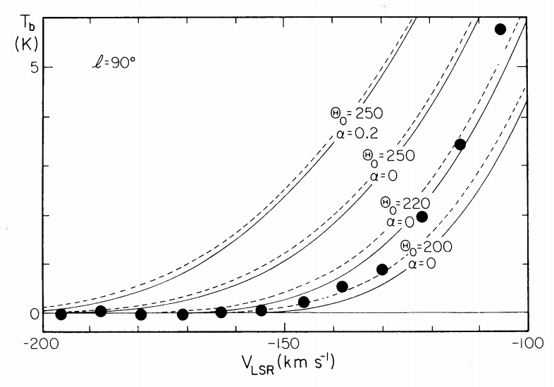
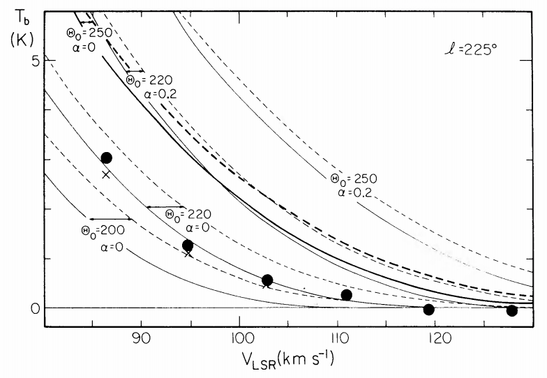
Figure 8.16: Observed HI intensity versus \(v_\mathrm{los}\) toward \(l=90^\circ\) and \(l=225^\circ\) compared to rotation curve models with different \(\Theta_0 =v_c(R_0)\) (Knapp et al. 1978).
We see that the intensity of HI emission (shown here as the brightness temperature \(T_b\)) agrees best with \(v_c(R_0) = 220\,\mathrm{km\,s}^{-1}\) in both of these directions. Based on this good agreement, this has been the standard value of \(v_c(R_0)\) for the last 40 years (Kerr & Lynden-Bell 1986). But the value of \(v_c(R_0)\) continues to be debated until this day and it is clear that this HI-based measurement is not unambiguous. Modern determinations of \(v_c(R_0)\) are made using, among others, the observed kinematics of disk stars based on dynamical-modeling techniques that we introduce in the next few chapters or using modeling of tracers in the stellar halo along the lines that we discussed in Part I.
The most important property of Equation (8.23) is that for rings inside the solar circle, the \((l,v)\) distribution terminates at a positive velocity for \(l > 0\) and a negative value for \(l < 0\). This terminal point at a given \(l\) is where a ring of radius \(R_c = R_0\,|\sin l|\) reaches its extremum in \(l\). At that point, \(v_\mathrm{los}\) is \begin{equation}\label{eq-vterm} v_\mathrm{los, term}(l\in[-90^\circ,90^\circ]) = \left[\Omega(R_0\,|\sin l|)-\Omega(R_0)\right]\,R_0\,\sin l\,. \end{equation} Because this is the locus on which the \((l,v)\) diagram ends or “terminates”, this is known as the terminal velocity curve. Because the terminal velocity is that along the line of sight where the line of sight is tangent to the circle with \(R_c = R_0\,|\sin l|\), this method is also known as the tangent-point method. We can measure the terminal velocity as a function of \(l\) by delineating the line at which the \((l,v)\) distribution ends (because the terminal-velocity curve consists of gas inside of the solar circle, there is no reason to think that there would be no gas observed at this terminal curve, which is different from the “final curve” at large \(R\) that we discussed above). With measurements of \(v_\mathrm{los, term}(l)\) in hand, we can then determine the rotation curve from Equation (8.24) \begin{equation}\label{eq-vterm-vc} v_c(R) = \pm v_\mathrm{los, term}(l) + v_c(R_0)\,\frac{R}{R_0}\,, \end{equation} where \(l = \pm\mathrm{arcsin}(R/R_0)\). Each value of \(|l|\) gives two independent estimates of \(v_c(R)\). Equation (8.25) is one of the main methods with which the Milky Way’s rotation curve has been determined at \(R < R_0\).
We can directly compare the terminal velocity curve for different potentials with the observed \((l,v)\) distribution. In Figure 8.17, we do this for three rotation curve: a flat rotation curve \(v_c(R) = \mathrm{constant}\), a solid-body rotation curve \(v_c(R) = \Omega\,R\), and the rotation curve for a razor-thin exponential disk with \(R_d = 3\,\mathrm{kpc}\). We use \(v_c(R_0) = 220\,\mathrm{km\,s}^{-1}\) for all three rotation curves.
[10]:
figure(figsize=(10,5),dpi=300)
data= gmc_plot_lv(rasterized=True)
ylim(-225.,225.)
ro= 8.*u.kpc
vo= 220.*u.km/u.s
lp= potential.LogarithmicHaloPotential(normalize=1.,
                                       vo=vo,ro=ro)
ls= numpy.linspace(-numpy.pi/2.,numpy.pi/2.,101)*u.rad
line_flat= plot(ls.to(u.deg),lp.vterm(ls).to(u.km/u.s),lw=3.,
               label=r'$v_c(R) = \mathrm{constant}$')
# size R of homogeneous >> considered region
hp= potential.HomogeneousSpherePotential(normalize=1.,R=10.,
                                         vo=vo,ro=ro)
line_solid= plot(ls.to(u.deg),
                 u.Quantity([hp.vterm(l).to(u.km/u.s) for l in ls]),
                 lw=3.,
                 label=r'$\Omega(R) = \mathrm{constant}$')
rp= potential.RazorThinExponentialDiskPotential(normalize=1.,
                                                hr=3.*u.kpc,
                                               vo=vo,ro=ro)
ls= numpy.linspace(0.,numpy.pi/2.,101)*u.rad
line_rp= plot(ls.to(u.deg),rp.vterm(ls).to(u.km/u.s),lw=3.,
             label=r'$v_c(R) = \mathrm{exp.\ disk}$')
plot(-ls.to(u.deg),-rp.vterm(ls).to(u.km/u.s),lw=3.,
     color=line_rp[0].get_color())
legend(handles=[line_flat[0],line_solid[0],
               line_rp[0]],
       fontsize=18.,loc='upper left',frameon=False);

Figure 8.17: The terminal velocity curve for different rotation-curve models overlaid on the longitude-velocity diagram from Figure 8.14.
As expected, the solid-body rotation curve is zero everywhere (remember that solid-body rotation keeps all relative line-of-sight velocities zero within a disk) and it is clear that gas in the Milky Way does not rotate as a solid body. The terminal velocity curve from the razor-thin exponential disk turns over around \(l=20^\circ\), which is not observed in the distribution. The terminal velocity curve of a flat rotation curve rises toward \(l=0\) (from the side of positive \(l\)) in a similar way as observed in the data. We should not over-interpret this good agreement, because it is somewhat accidental: within \(\approx R_0\,\sin 30^\circ = 4\,\mathrm{kpc}\), the Galactic bar dominates the potential and gas is not on circular orbits as we assumed in the derivation so far, so we cannot directly interpret the observed terminal velocity curve at \(|\sin l| < 1/2\) in terms of the rotation curve of an axisymmetric disk (e.g., Chemin et al. 2015).
So far we have only discussed the effect of axisymmetric galactic rotation on the observed \((l,v)\) diagram. Looking more closely at the \((l,v)\) diagrams of HI and of the molecular gas, we see that there are significant overdensities in it. We have explained one of these as the signature of a ring of molecular gas, but others cannot be interpreted in terms of rings and even the ring that we purportedly explained looks distinctly asymmetric in \(l\). Many of these overdensities can be explained through the effect of spiral structure on the gas kinematics, but we will not discuss that further.

 .
. .
. .
.