
6.4. The mass of the Milky Way’s dark matter halo
Given that we know, from, e.g., the escape velocity near the Sun and from the Local Group timing argument, that the Milky Way disk must be surrounded by a massive halo of dark matter, we would like to find out more about its mass profile. Because the disk only extends out to about 15 kpc from the center, any dynamical analysis that wants to determine the mass profile at larger distances must use non-disk tracers, such as globular clusters (see Chapter 5.2) or stars orbiting in the stellar halo. The simplest assumption is that the dark-matter halo is spherical and that it dominates the mass outside of the disk, such that the total potential is also approximately spherical. Then we can use the spherical Jeans equation.
We derived the spherical Jeans equation in Chapter 5.4. Let’s write the spherical Jeans equation (5.48) in terms of the circular velocity rather than the enclosed mass \begin{equation}\label{eq-spher-jeans-anisotropy-vc} v_c^2(r) = -\sigma_r^2\,\left(\frac{\mathrm{d} \ln (\nu\,\sigma_r^2)}{\mathrm{d} \ln r} + 2\,\beta\right)\,. \end{equation} Therefore, to observationally determine the circular velocity curve \(v_c(r)\) using the spherical Jeans equation in the Milky Way, we need to measure \(\nu(r)\), \(\sigma_r(r)\), and \(\beta(r)\) of the tracer population that we are using. It is possible to measure \(\nu(r)\) for large photometric samples of halo stars (e.g., Bell et al. 2008). Because obtaining large data samples with three-dimensional velocities is hard, even in the era of Gaia, determining \(\sigma_r(r)\) and especially \(\beta(r)\) is more difficult. At large \(r\) (\(r \gg R_0\), the solar radius), \(\sigma_r(r)\) is approximately equal to \(\sigma_\mathrm{los}(r)\), because to a good approximation the Sun is sitting at the center of the Galaxy in this case and therefore \(v_\mathrm{los} \approx v_r\). For the same reason, measuring \(\beta(r)\) requires tangential velocities (i.e., proper motions).
Xue et al. (2008) presented a sample of \(\approx 2,400\) blue-horizontal branch (BHB) stars from SDSS with well-measured distances and \(v_\mathrm{los}\). They analyzed these primarily by comparing them to a cosmological simulation, but also applied a simple Jeans analysis that agreed with the more complex analysis. For the SDSS survey volume, they found that \(\sigma_r(r) \approx \sigma_\mathrm{los}(r)\) to good accuracy. From the large sample of BHB stars, they could precisely determine \(\sigma_\mathrm{los}\) and found it to be slowly declining with radius as \begin{equation} \sigma_\mathrm{los}(r) = \left(111\pm1\,\mathrm{km\,s}^{-1}\right)\,\exp\left(-\frac{r}{354^{+91}_{-60}\,\mathrm{kpc}}\right)\,. \end{equation} They combined this with \(\nu(r) \propto r^{-3.5}\) in Equation (6.12) to determine \(v_c(r)\) using \(\beta = 0\) as the simplest, isotropic assumption and using \(\beta = 0.37\), as informed by numerical simulations. Before discussing the results in more detail, we note that both choices lead to \(v_c \approx 200\,\mathrm{km\,s}^{-1}\) and we estimate the uncertainty in \(v_c\) coming from our lack of knowledge of \(\beta\) (a manifestation of the mass–anisotropy degeneracy). From Equation (6.12) we have that \begin{equation}\label{eq-Xue-beta-depend} \Delta v_c \approx -\sigma_r^2\,\beta/v_c \approx -62\,\beta\,\mathrm{km\,s}^{-1}\,, \end{equation} using \(\sigma_r \approx 111\,\mathrm{km\,s}^{-1}\) and \(v_c \approx 200\,\mathrm{km\,s}^{-1}\).
The rotation curve \(v_c(r)\) derived from the Jeans equation in the form (6.12) by Xue et al. (2008) is shown in Figure 6.1.
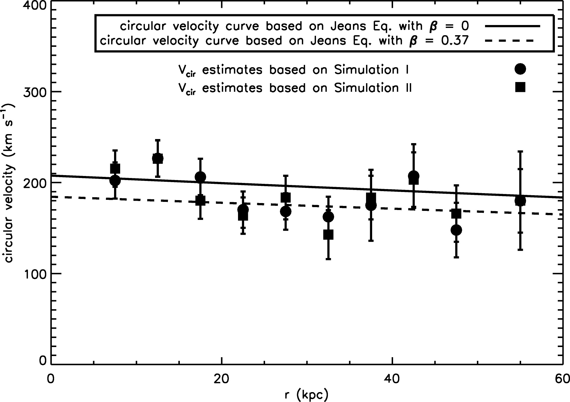
Figure 6.1: The Milky Way’s circular velocity in the halo from Xue et al. (2008).
The solid line shows the derived rotation curve when \(\beta = 0\), while the dashed line uses \(\beta = 0.37\). From Equation (6.14), we expect \(\Delta v_c \approx -23\,\mathrm{km\,s}^{-1}\) and approximately constant across the radial range, which agrees with this figure. Because the uncertainty in \(\beta\) mostly gives rise to a constant offset (unless \(\beta(r)\) has a strong radial variation), the slope of \(v_c(r)\) is robust. The best-fit circular velocity profile is declining, which implies that the mass density declines faster than \(r^{-2}\), as expected for dark-matter halos from cosmological simulations.
Equation (6.14) makes it clear that the anisotropy parameter \(\beta\) has a large effect on the rotation curve that we derive from the halo BHB kinematics. Much effort is therefore going towards determining \(\beta\). For example, Deason et al. (2013) used Hubble-Space-Telescope proper motions for a few halo stars to determine \(\beta = 0.0^{+0.2}_{-0.4}\) around \(r = 25\,\mathrm{kpc}\), indicating that the halo is approximately isotropic in that range. However, the anisotropy in the solar neighborhood has long been known to be strongly radial (e.g., \(\beta \approx 0.5\); Morrison et al. 1990), albeit with a strong metallicity dependence that has a more isotropic distribution at the metallicities of the Xue et al. (2008) BHB stars (e.g., Belokurov et al. 2018). A detailed investigation of the anisotropy out to 100 kpc as a function of metallicity using LAMOST and Gaia data finds a constant anisotropy out to \(r \approx 25\,\mathrm{kpc}\) followed by a linear drop to \(\beta \approx 0.2\) at \(r\approx 100\,\mathrm{kpc}\) (Bird et al. 2019). For the metallicities of the Xue et al. (2008) BHB stars, they find the \(r \lesssim 25\,\mathrm{kpc}\) plateau to lie at \(\beta \approx 0.7\), dropping to about \(\beta \approx 0.4\) at \(r \approx 60\,\mathrm{kpc}\). For this \(\beta(r)\) profile, the rotation curve in Figure 6.1 above would be another \(\Delta v_c \approx 20\,\mathrm{km\,s}^{-1}\) lower at \(r \lesssim 25\,\mathrm{kpc}\) and then be closer to flat to end up at about the same \(v_c\) at \(r =60\,\mathrm{kpc}\).
Because \(v_c^2 = G\,M(<r)/r\), we can model the data in Figure 6.1 with a mass model for the Milky Way. Xue et al. (2008) do this with a simple disk+bulge+halo model, where the disk is modeled as a spherical potential with an exponential density (what could be called the “spherical-cow disk model”). From this they find \(M(<60\,\mathrm{kpc}) = 4.0\pm0.7\times10^{11}\,M_\odot\) and a total mass \(M_\mathrm{MW} = 1.0\pm0.3\times10^{12}\,M_\odot\). This is similar to the total halo mass found from the local escape velocity in Section 6.2 above.

 .
. .
. .
.