
6.8. Estimating masses with multiple populations: cusps vs. cores in dwarf spheroidals
Let us now return to the problem of determining the inner dark-matter profile in dwarf spheroidal galaxies around the Milky Way and introduce a powerful idea in equilibrium dynamical modeling: tracer populations with different spatial distribution and kinematics should give consistent and complimentary determinations of the mass profile. That is, all tracer populations in a given galaxy are orbiting in the same gravitational potential and equilibrium modeling of their density and kinematics should give the same resulting mass profile. This principle could be used, for example, to test the assumption of equilibrium dynamics: if two tracer populations give inconsistent mass distributions, this could be because they are not both in dynamical equilibrium. But we have also seen above that tracer populations measure the mass profile best at a radius determined by their spatial distribution (\(r_3\) for the Wolf estimator). If different tracer populations have very different spatial distributions, they will best determine the mass at different positions, which allows us to robustly build up a mass profile by combining different populations.
One application of this general idea was presented by Walker & Peñarrubia (2011) in the case of dSphs. In Section 6.5 above, we saw how Jeans modeling of the kinematics of Milky Way dSphs allowed their masses to be determined, but we also saw that the degeneracy between mass and anisotropy did not allow strong constraints on the inner density slopes of the mass profile to be derived. Figure 6.7 shows another example of this, from Jeans models of the Fornax dSph.
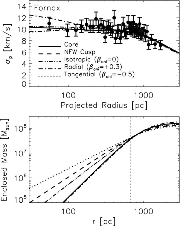
Figure 6.7: Enclosed-mass profile of Fornax from Jeans modeling (Walker & Peñarrubia 2011).
Even though there is lots of data on the velocity dispersion at different radii, the data is consistent with either a cored or a cuspy profile and the difference between cored and cuspy is similar to the range spanned by models with different values of \(\beta\). The bottom panel of the figure above again shows that all of the different mass and \(\beta\) models agree on the enclosed mass within the half-mass radius.
Spectroscopic studies of dSphs around the Milky Way have shown that these galaxies consist of multiple sub-populations with different chemical abundances and density profiles. For example, Tolstoy et al. (2004) found two populations in the Sculptor galaxy, with a centrally-concentrated metal-rich population, and a more diffuse metal-poor population. Similar studies of other dSphs have shown similar results. This presumably happens because these populations form at different times in the life of the dSph, when star-formation is happening on different spatial scales. Because these sub-populations have different spatial distributions, they have different \(R_e\) and \(r_{1/2}\) and will therefore measure the enclosed mass at different radii (see Equation 6.28). Therefore, conceptually we can proceed as follows: obtain spectroscopic data for many stars in dSphs, split them into distinct chemical populations using their chemical abundances, and obtain the enclosed mass \(M(<r_{1/2,i})\) at the different \(\{r_{1/2,i}\}\) of these populations. The profile \([r_{1/2,i},M(<r_{1/2,i})]\) is then a robust measurement of the mass profile and we can, for example, determine the slope \(\Gamma = \mathrm{d} \ln M / \mathrm{d} \ln r\).
An analysis of this sort was performed by Walker & Peñarrubia (2011) for the Carina, Sculptor, and Fornax dSphs, although the details of the implementation are slightly more complicated than what we have presented here. For Carina they did not find evidence for two distinct sub-populations and they could therefore only determine the mass at a single radius. But for Sculptor and Fornax they were able to probabilistically split the data into two populations, determine \(M(<r)\) at two different radii, and constrain \(\Gamma\). Their results are displayed in Figure 6.8.
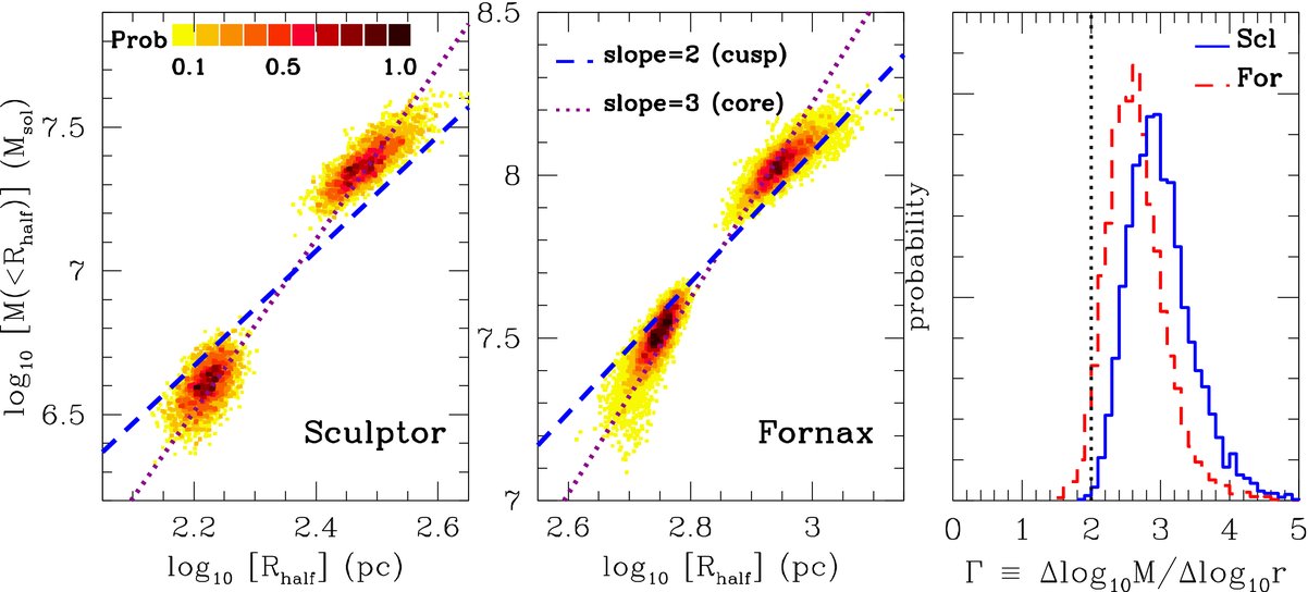
Figure 6.8: Inner dark-matter profile of Fornax from applying a Wolf-like mass estimator to two stellar populations with different half-mass radius (Walker & Peñarrubia 2011).
From the definition of \(\Gamma\), it is clear that a cored profile with \(\rho(r) \propto \mathrm{constant}\) would give \(M(<r) \propto r^3\) and therefore \(\Gamma = 3\), while a cuspy profile \(\rho(r) \propto 1/r\) would give \(M(<r) \propto r^2\) and \(\Gamma = 2\). The data are inconsistent with a cuspy profile at the 95% (for Sculptor) to 99.8% confidence level (for Fornax).
Using simple equilibrium dynamical modeling applied to two tracer sub-populations, we can therefore robustly determine the inner dark-matter slopes of dSphs and rule out that these have the cuspy profile expected from cosmological simulations of the formation of dark matter halos. Instead, these dark-matter halos appear to have constant-density cores with sizes of a few hundred parsecs. This could be because the popular cold-dark-matter model is incorrect or it could result from gravitational interactions between the few stars that these dwarf galaxies contain and the dark matter in their centers. In particular, enough of the energy released in explosions of massive stars as supernovae might be transferred as gravitational energy to the dark matter distribution (this is a type of baryonic feedback; see Chapter 19.3.3). For such gravitational-energy injection to significantly change the phase-space density of dark matter, it has to happen non-adiabatically, that is, on time scales that are short with respect to the dynamical time.
We can explore how non-adiabatic energy injection can destroy a central dark-matter cusp and turn it into a core using the tools from Chapter 5. In particular, we can model the dark-matter distribution in a dSph with an isotropic Hernquist distribution, for which we determined the equilibrium distribution function in Chapter 5.6.1. Let’s use Fornax as an example. We model Fornax as an isotropic Hernquist profile with a total mass \(M = 3\times 10^8\,M_\odot\) and a scale radius \(a = 1\,\mathrm{kpc}\). We then sample this profile with \(10^6\) particles:
[6]:
from galpy.potential import HernquistPotential
from galpy.df import isotropicHernquistdf
totmass= 3.*1e8*u.Msun
hp= HernquistPotential(amp=2.*totmass,a=1.*u.kpc)
dfh= isotropicHernquistdf(pot=hp)
samp= dfh.sample(n=int(1e7))
Next we want to inject gravitational energy in this sample in a non-adiabatic way. We will do this by perturbing all of the velocities with perturbation velocities drawn from an isotropic Gaussian distribution characterized by a dispersion \(\sigma\). This mimics non-adiabatic heating. This instantaneous heating places the system out of equilibrium, so we integrate all orbits for 500 Myr to see what new equilibrium state the system settles in. Integrating all \(10^6\) particles would take a long time, so we only consider a subsample. Because we want to focus on what will happen in the inner regions, we sample approximately equal numbers in equal logarithmic bins in radius. The following code does this subsampling and orbit integration, and it computes the weights of each subsampled particle such that they faithfully represent the underlying phase-space density:
[39]:
# Assumes that n << samp.size
def logr_sample(samp,n):
    return samp[numpy.random.choice(numpy.arange(samp.size),size=n,replace=False,
                                    p=1./samp.r()/numpy.sum(1./samp.r()))]
subsamp= logr_sample(samp,100_000)
subsamp_weight= subsamp.r()/(numpy.sum(subsamp.r()))\
        *totmass.to_value(u.Msun)
ts= numpy.linspace(0.,0.5,101)*u.Gyr
subsamp.integrate(ts,hp,method='dop853_c')
We can compare the density profile of the original sample to that of the subsample at \(t=0\) and after 500 Myr. All agree well with the analytical profile, to within the sampling noise as demonstrated in Figure 6.9.
[40]:
bins= 80
def plot_sample_density(samp,bins,weights,rrange=None,r_plot_unit=u.pc,
                       label=None):
    w,e= numpy.histogram(numpy.log(samp.r().to_value(u.pc)),
                         bins=bins,range=rrange,weights=weights)
    binrs= numpy.exp((numpy.roll(e,-1)+e)[:-1]/2.)
    ploty= w/(4.*numpy.pi*binrs**3.*(e[1]-e[0]))
    loglog(binrs*(u.pc/r_plot_unit).to(u.dimensionless_unscaled),
           ploty,drawstyle='steps-mid',label=label)
    return binrs*u.pc

figure(figsize=(7,5))
plotrs= plot_sample_density(samp,bins,
                            totmass*numpy.ones(samp.size)/samp.size,
                            r_plot_unit=u.kpc,
                            label=r'$\mathrm{Full\ original\ sample}$')
plot_sample_density(subsamp,bins,subsamp_weight,r_plot_unit=u.kpc,
                    label=r'$\mathrm{Original\ subsample}$')
plot_sample_density(subsamp(ts[-1]),bins,subsamp_weight,r_plot_unit=u.kpc,
                    label=r'$\mathrm{Subsample\ after\ 500\ Myr}$')
plot(plotrs.to(u.kpc),hp.dens(plotrs,0.),color='k',
    label=r'$\mathrm{Analytical\ Hernquist\ profile}$')
xlabel(r'$r\,(\mathrm{kpc})$')
ylabel(r'$\rho\,(M_\odot\,\mathrm{pc}^{-3})$')
xlim(0.01,100)
ylim(1e-9,3e1)
gca().xaxis.set_major_formatter(FuncFormatter(
                lambda y,pos: (r'${{:.{:1d}f}}$'.format(int(\
                    numpy.maximum(-numpy.log10(y),0)))).format(y)))
legend(frameon=False,fontsize=18.);

Figure 6.9: Original and evolved samples from a Hernquist profile.
Next we heat the particles in the subsample, by adding velocities drawn from an isotropic Gaussian. To mimic that this heating only happens in the inner part of the galaxy where stars are abundant, we only heat stars within 1 kpc:
[41]:
from galpy.orbit import Orbit
from galpy.util import coords
def heat_orbits(samp,sigma,rmax):
    new_vx= samp.vx()+numpy.random.normal(size=samp.size)*sigma*(samp.r() < rmax)
    new_vy= samp.vy()+numpy.random.normal(size=samp.size)*sigma*(samp.r() < rmax)
    new_vz= samp.vz()+numpy.random.normal(size=samp.size)*sigma*(samp.r() < rmax)
    new_vR, new_vT, _= coords.rect_to_cyl_vec(new_vx,new_vy,new_vz,
                                              samp.R(),samp.phi(),samp.z(),
                                              cyl=True)
    return Orbit([samp.R(),new_vR,new_vT,samp.z(),new_vz,samp.phi()])
def heat_subsample(samp,sigma,rmax):
    heated_subsamp= heat_orbits(subsamp,sigma,rmax=1.*u.kpc)
    ts= numpy.linspace(0.,.5,101)*u.Gyr
    heated_subsamp.integrate(ts,hp)
    return heated_subsamp
We then compare the resulting density distribution for different levels of heating in Figure 6.10 (note that the velocity dispersion of the dark matter is \(\approx 10\,\mathrm{km\,s}^{-1}\) for the unperturbed system).
[42]:
figure(figsize=(7,5.5))
plotrs= plot_sample_density(subsamp(ts[-1]),bins,subsamp_weight,
                            r_plot_unit=u.kpc,
                            label=r'$\mathrm{Heating}\ \sigma = 0$')
heated_subsamp= heat_subsample(subsamp,10.*u.km/u.s,rmax=1.*u.kpc)
plotrs= plot_sample_density(heated_subsamp(ts[-1]),bins,subsamp_weight,
                            r_plot_unit=u.kpc,
                            label=r'$\mathrm{Heating}\ \sigma = 10\,\mathrm{km\,s}^{-1}$')
heated_subsamp= heat_subsample(subsamp,20.*u.km/u.s,rmax=1.*u.kpc)
plotrs= plot_sample_density(heated_subsamp(ts[-1]),bins,subsamp_weight,
                            r_plot_unit=u.kpc,
                            label=r'$\mathrm{Heating}\ \sigma = 20\,\mathrm{km\,s}^{-1}$')
heated_subsamp= heat_subsample(subsamp,40.*u.km/u.s,rmax=1.*u.kpc)
plotrs= plot_sample_density(heated_subsamp(ts[-1]),bins,subsamp_weight,
                            r_plot_unit=u.kpc,
                            label=r'$\mathrm{Heating}\ \sigma = 40\,\mathrm{km\,s}^{-1}$')
plot(plotrs.to(u.kpc),hp.dens(plotrs,0.),color='k',
    label=r'$\mathrm{Analytical\ Hernquist\ profile}$')
xlabel(r'$r\,(\mathrm{kpc})$')
ylabel(r'$\rho\,(M_\odot\,\mathrm{pc}^{-3})$')
xlim(0.01,100)
ylim(1e-9,3e1)
gca().xaxis.set_major_formatter(FuncFormatter(
                lambda y,pos: (r'${{:.{:1d}f}}$'.format(int(\
                    numpy.maximum(-numpy.log10(y),0)))).format(y)))
legend(frameon=False,fontsize=18.);

Figure 6.10: Hernquist profiles heated by feedback in the inner kpc.
We see that the heating indeed causes a core to form (the density in the center becomes constant with radius) and that the size of the core depends on the amount of heating applied, with larger values corresponding to larger cores. Thus, to create a core with a size of a few hundred pc, we need to heat the dark-matter distribution by \(\approx 20\,\mathrm{km\,s}^{-1}\).
The standard explanation for the source of this heating (e.g., Pontzen & Governato 2012) is that it comes from the non-adiabatic changes in the stellar-mass profile that result from repeated supernova explosions of massive stars. Thus, eventually, the source of this gravitational energy has to be related to the energy released by supernovae of massive stars. The total amount of gravitational energy required is \(\approx M(r<1\,\mathrm{kpc})\,\sigma^2 /2 \approx 3\times 10^{53}\,\mathrm{erg}\) (this estimate agrees well with more sophisticated treatments, e.g., Peñarrubia et al. 2012). We can compare that number to the total amount of energy released by supernovae in Fornax, which has a stellar mass of \(\approx 3\times 10^7\,M_\odot\), corresponding to about \(10^8\) stars. According to the standard Kroupa (2001) initial mass function, 0.37% of stars have high enough mass (\(M > 8\,M_\odot\)) to explode as a supernova, or about \(3.7\times 10^5\) for the total stellar population of Fornax. Each supernova releases about \(10^{51}\,\mathrm{erg}\), or a total of \(3.7\times 10^{56}\,\mathrm{erg}\) for Fornax’s stars. Thus, there is plenty of energy released in supernovae available for heating the dark-matter gravitational potential and even transferring only a fraction of 1% of the energy released in supernovae to the dark-matter distribution is enough to turn the cusps predicted by the standard cold-dark-matter paradigm into the observed cores.

 .
. .
. .
.