
8. Gravitation in galactic disks
So far, we have studied orbits and equilibria of spherical mass distributions in detail. We have seen that orbits in such mass distributions are rather simple, because the spherical symmetry leads to the conservation of angular momentum. This means that the orbital plane is fixed for any orbit and that the motion within that plane is also constrained by the conservation of the component of the angular momentum perpendicular to the plane. For static spherical mass distributions, the conservation of energy gives a further strong constraint and closed orbits become quite simple: orbiting bodies oscillate in the radial direction between a close (pericenter) and far (apocenter) point from the center, while “looping” around the center in the azimuthal direction in a fixed direction (either clockwise or counter-clockwise). These radial and azimuthal oscillations are characterized by a radial and azimuthal frequency, which are typically not commensurate and orbits do not close. But for any reasonable galactic potential bodies will perform between 1 and 2 radial oscillations for each loop around the center. In the previous two chapters we discussed the dynamical equilibria in spherical potentials: because of the many conserved quantities, these equilibria are also rather simple. Despite their simplicity, we learned many properties of the mass distributions of approximately spherical galactic systems in the previous chapter: the Milky Way halo, dwarf spheroidals, and ultra-faint dwarf galaxies.
However, many of the galactic systems that we are interested in studying are manifestly non-spherical, but are much better approximated as flat disks. See the following examples:
|
|


(Credit: NGC 5907: NASA/JPL-Caltech/M.L.N. Ashby (Harvard-Smithsonian CfA); M31: NASA/JPL-Caltech)
These are just two examples of large disk galaxies: NGC 5907 and M31 (our nearest large neighbor). Our own Milky Way is another example of a disk galaxy. Disk galaxies are ubiquitous in the Universe, making up about half of all large galaxies in the local Universe. Because these galaxies deviate strongly from spherical symmetry, they are not well described by the framework that we introduced in the previous few chapters and using the spherical approximation as a starting point is not a good approach for most properties in disk potentials. In particular, orbits and the dynamical equilibria of orbits can be quite a bit more complicated than those in spherical potentials. In this part, we therefore focus on the structure and dynamics of disk galaxies. We start on this in this chapter by discussing the observed structure of disk galaxies in more detail. Then we describe techniques for finding good gravitational potentials that describe these disk mass distributions, with a particular emphasis on mass distributions that are axisymmetric—meaning that they are symmetric with respect to rotations around the axis perpendicular to the disk. Such mass distributions are most easily described in cylindrical coordinates. Therefore, we write the density as \(\rho(R,\phi,z)\) for general densities and \(\rho(R,z)\) for axisymmetric densities (which do not depend on \(\phi\)); potentials are written as \(\Phi(R,\phi,z)\) in general and \(\Phi(R,z)\) for axisymmetric potentials.
An axisymmetric approximation to a disk galaxy ignores the effect of, e.g., bars or spiral structure. We will see there that those features can be well described as perturbations to the overall axisymmetric description. Ellipsoidal distributions that are closer to spherical but non-axisymmetric require a different approach, because they are not well approximated as disks; we discuss the properties of triaxial, ellipsoidal potentials more in the next part, starting in Chapter 13.
8.1. The observed structure of disk galaxies
We briefly introduced the structure of disk galaxies in Chapter 2.2. To motivate our discussion of good mass models for disk galaxies, we look at the observations in a little more detail first.
As discussed in Chapter 2.2.1, the radial surface-brightness profile of disk galaxies is overall well described by an exponential function:
Thus, we say that galactic disks are exponential disks. Many decades have passed since Freeman (1970)’s paper in which he first described the exponential nature of galactic disks and we now have photometry for millions of galaxies from surveys such as the Sloan Digital Sky Survey (SDSS) that allow us to investigate the exponential nature of the light distribution in detail. The following picture shows the main different types of profiles for disk galaxies:

(Credit: Pohlen & Trujillo 2006; left panels: r’-band SDSS cut-outs (ellipse: noise limit \(\approx 140\) arcsec); right panels: azimuthally averaged, radial surface-brightness profiles in g’ (triangles) and r’ (circles) with a fit in black.)
The galaxy shown in the top panels, NGC 2776, has a pure exponential profile (known as a type I profile): an exponential decline without any change of (logarithmic) slope from the center to the very outskirts of the galaxy, except for a small central concentration. The other panels display galaxies with more complicated profiles, either a break towards a steeper decline in the outer parts of the galaxy (type II profiles) or a break to a more shallow profile (type III). While there are these different types, the main thing to remember is that all galactic disks have to first approximation exponential profiles.
To take observations of the surface-brightness profiles of disk galaxies and jump to the conclusion that the distribution of stellar mass in disks declines exponentially requires an additional assumption. We have to assume that stellar mass traces observed luminosity with a constant scaling, the mass-to-light ratio. This allows us to convert the observed luminosity to stellar mass and determine the mass profile. The mass-to-light ratio is normally expressed in solar units of (solar mass)/(solar luminosity) and is typically a few in these units. Like other units in astronomy (I’m looking at you log g!), this unit is often dropped and the mass-to-light ratio is specified as, for example, \(M/L = 3\). From models for the relative proportion of different stars born from a molecular cloud in a star-formation event (the initial mass function) and models of stellar evolution, we can compute theoretical mass-to-light ratios. These are typically a few, but vary somewhat for different bands, which is ultimately caused by the fact that light is a very biased tracer of mass: the light in most bands is dominated by luminous, relatively high-mass stars (mass of the Sun or higher), while the mass budget is dominated by the lowest mass stars (far below the mass of the Sun). It is therefore not obvious that the stellar mass profiles of disks are also exponential.
Without going into much more detail, we will just note that in the Milky Way we can measure the amount of mass contained in the disk directly at different distances from the Galactic center. The following shows the surface-mass density as a function of radius as opposed to the surface-brightness profile that we discussed above:

(Credit: Bovy & Rix 2013)
This surface-mass profile is very well represented by an exponential and it therefore does seem to be the case that the stellar mass distribution itself is exponential and that mass-to-light ratios cannot vary too much with radius. But this disconnect between mass and light is important to keep in mind in all of the discussions of mass distributions in this book.
In Chapter 2.2.1, we also discussed how the distribution of stars in the direction vertical to the disk plane is well described by a \(\mathrm{sech}^2\) profile. In cylindrical coordinates, the vertical direction is denoted as \(z\) and the \(\mathrm{sech}^2\) profile is:
where \(h_z\) is a parameter called the scale height. An example of the vertical profile of a disk galaxy is furnished by the observations of NGC 4244 already discussed in Chapter 2.2.1:

(Credit: van der Kruit & Freeman 2011; NGC 4244: top: a pure-disk galaxy seen edge-on; bottom: vertical surface-brightness profiles at a range of distances from the center [profiles are displaced along the X axis to avoid overlap])
At distances \(z \gg h_z\), the profile becomes
Thus, the profile becomes an exponential with an exponential scale height equal to \(h_z\). Ignoring the detailed density profile near the mid-plane, a simple, axisymmetric approximation to the number density profile \(n(R,z)\) in disk galaxies is therefore that they are exponential both in radius \(R\) and height \(|z|\) with scale lengths/heights \(h_R\) and \(h_z\):
This is the double-exponential disk profile. In principle, the scale height \(h_z\) could depend on the radial position \(R\), but many observations like the one shown above demonstrate that at least the overall thickness of the stellar mass distribution in disk galaxies is constant with \(R\), thus, the double-exponential disk profile is an excellent approximation of the stellar density distribution in a typical disk.
In the Milky Way and near the Sun we can measure the vertical profile of stars in exquisite detail. Unlike in most external galaxies, in the Milky Way we can count individual stars and are therefore not limited to making sense of the integrated light of stars (which is dominated by rare, luminous stars). The following three panels display the vertical number density of stars near the Sun from SDSS:

(Credit: Jurić et al. 2008)
The different panels show different vertical ranges, with the top panel the closest to the midplane. Stars with different colors r-i are used to determine the number counts at different heights: the redder stars are dimmer and, in a magnitude-limited survey such as SDSS, found closer to the Sun (which sits close to the midplane); the bluer stars are brighter and can be seen to multiple kpc (bottom panel). The top panel shows that the number density is close to exponential within a few 100 pc, although the middle panel shows a turnover towards a shallower profile (sometimes called a “thick disk”, although the author of this book strongly disagrees with this terminology; Bovy et al. 2012). Even though the stellar profile looks perfectly exponential in the top panel, detailed number counts within 100 pc of the midplane demonstrate that the stellar profile flattens as it reaches the midplane (Bovy 2017b; Bennett & Bovy 2019).
Thus, to a first approximation, we can model the stellar mass distribution in disk galaxies using the double-exponential disk profile. Depending on the context, the most important deviations from this profile are that (a) near the disk mid-plane the vertical density flattens and is better described as a \(\mathrm{sech}^2\) profile, (b) far from the mid-plane the vertical density requires at least another, thicker exponential component to account for the detailed vertical distribution of stars of different ages, and (c) the radial profile may deviate from the pure exponential profile in the inner or outer ranges of the disk.
8.2. Simple gravitational potentials for flattened mass distributions
Determining the gravitational potential for general flattened mass distributions is difficult. Newton’s theorems, which we discussed in Chapter 3.2, do not hold for flattened systems and we can therefore not proceed in the same manner as we did for spherical mass distributions (where we could add the potential from concentric, spherical shells to build up the total potential for any spherical mass distribution). To illustrate the complication, we compare the gravitational potential from a thin spherical shell with that of a thin ring of the same total mass in the following figure (we compare the potentials along \(z = 0.1\,R\) to avoid a singularity that exists when actually crossing through the ring at \(z=0\); we will discuss how the actually compute the potential and force due to a ring of matter below):
[4]:
from galpy.potential import SphericalShellPotential, RingPotential
figsize(8,6)
sp= SphericalShellPotential(amp=1.,a=1.5)
rp= RingPotential(amp=1.,a=1.5)
rs= numpy.linspace(0.1,7.,101)
line_shell= galpy_plot.plot(rs,[sp(r,0.1*r) for r in rs],
                            yrange=[-1.,0.],
                            xlabel=r'$r$',
                            ylabel=r'$\Phi$',
                            label=r'$\mathrm{Shell}$')
line_ring= galpy_plot.plot(rs,[rp(r,0.1*r) for r in rs],overplot=True,
                           label=r'$\mathrm{Ring}$')
legend(handles=[line_shell[0],line_ring[0]],
       fontsize=18.,loc='lower right',frameon=False);
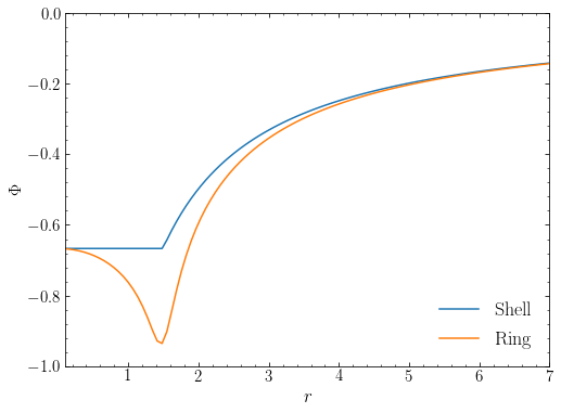
Unlike for the spherical shell, the potential within the ring is not constant and thus Newton’s first shell theorem does not hold (why the theorem doesn’t hold is clear from the geometric proof that we discussed in Chapter 3.2). The potential actually decreases with radius inside of the ring, implying that the gravitational force is pointing towards the closest side of the ring (why this is should again be clear from the geometric proof of Newton’s shell theorem). The following is a plot of the actual gravitational force, now at \(z=0\) to highlight the (integrable) singularity when passing through the ring:
[5]:
from galpy.potential import SphericalShellPotential, RingPotential
figsize(8,6)
sp= SphericalShellPotential(amp=1.,a=1.5)
rp= RingPotential(amp=1.,a=1.5)
rs= numpy.linspace(0.1,7.,101)
line_shell= galpy_plot.plot(rs,[sp.Rforce(r,0.) for r in rs],
                            yrange=[-1.,1.],
                            xlabel=r'$r$',
                            ylabel=r'$g_r$',
                            label=r'$\mathrm{Shell}$')
line_ring= galpy_plot.plot(rs,[rp.Rforce(r,0.) for r in rs],overplot=True,
                           label=r'$\mathrm{Ring}$')
legend(handles=[line_shell[0],line_ring[0]],
       fontsize=18.,loc='lower right',frameon=False);
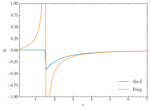
The amplitude of the force due to the ring within its plane is much higher than that of a shell and a ring of matter will therefore accelerate bodies within its plane more than a shell of the same mass. At large distances from the ring, the potential and force approach that of the spherical shell, which is the same as that of a point mass. This is a general rule for mass distributions of finite mass: at large distances their force becomes indistinguishable from that of a point of the same mass.
Thus, the potential of a ring is significantly different from that of a spherical shell. Because thin disks are more accurately approximated as consisting of rings rather than shells, their gravitational forces differ from those of spherical mass distributions in the same way that those of a ring differ from those of a shell: For a given mass, disks cause larger accelerations (and thus, e.g., velocities of a circular orbit) and the mass outside a given radius affects the gravitational acceleration felt by a body. We will discuss a general solution to determining the potential for any mass distribution below, but we will see that it is quite complicated, even in the limit that the distribution is axisymmetric and that the mass distribution is flattened into a zero thickness disk.
An easier method for obtaining gravitational potential models of flattened mass distributions is to posit a potential \(\Phi(R,z)\) (for an axisymmetric potentials) and then compute the corresponding density using the Poisson equation as \(\rho = \nabla^2 \Phi / (4\pi\,G)\). By not solving for the potential for a given density, but rather solving for the density corresponding to a given potential, we get around having to solve a partial differential equation. Naturally, this simplification comes at a cost: (i) we cannot choose the density distribution, but rather have to work with whatever we compute with \(\nabla^2 \Phi / (4\pi\,G)\) (this may not be a good enough model for the system that we are studying) and (ii) there is no guarantee that the density resulting from \(\rho = \nabla^2 \Phi / (4\pi\,G)\) is everywhere positive, so we may end up with a model that is unphysical in certain regions. Despite these issues, there are several useful, simple flattened gravitational potential models that are in wide-spread use and that we discuss in this section.
8.2.1. Razor-thin disk: The Kuzmin model
A simple flattened axisymmetric potential is that given by the following expression
with \(a \geq 0\) a parameter of the model. This potential resembles a point-mass potential \(\Phi(R,z) = -G\,M/\sqrt{R^2+z^2}\): for any \(z > 0\), Equation \(\eqref{eq-kuzmin-pot}\) is equivalent to the potential of a point-mass located at \((R,z) = (0,-a)\), while for any \(z < 0\), Equation \(\eqref{eq-kuzmin-pot}\) is equivalent to the potential of a point-mass located at \((R,z) = (0,a)\). Because the potential at any point \((R,z)\) with \(z \neq 0\) is equivalent to that of a point mass centered on a different point (which therefore has zero density at \((R,z)\)), the density corresponding to the potential in Equation \(\eqref{eq-kuzmin-pot}\) at any point with \(z \neq 0\) must be zero. This reasoning does not hold for points with \(z=0\): For those points, the potential is equivalent to a Plummer sphere, which has non-zero density everywhere (but the density at \(z=0\) is not that of a Plummer sphere, because the equivalence only holds for \(z=0\) exactly, and not for \(z=\epsilon\) and therefore not for the derivatives of the potential). The density corresponding to the potential in Equation \(\eqref{eq-kuzmin-pot}\) is therefore of the form
where \(\delta(z)\) is the Dirac delta function (Appendix B.1.1). This represents a zero-thickness disk or a razor-thin disk. The function \(\Sigma(R,\phi)\) is the surface density, which has units of mass over length squared. For the potential in Equation \(\eqref{eq-kuzmin-pot}\) the density will clearly be axisymmetric and, thus, \(\Sigma(R,\phi) = \Sigma(R)\).
To determine the relation between the surface density \(\Sigma(R)\) and the potential for any razor-thin disk, we integrate the Poisson equation over a volume \(\mathcal{V}\)
and plug in Equation \(\eqref{eq-razorthin-dens}\), switching to cylindrical coordinates
We can use the divergence theorem to write the volume integral on the left-hand side as an integral over the surface \(\mathcal{S}\) of the volume \(\mathcal{V}\). Then this becomes
were \(\mathrm{d}\mathcal{S}\cdot\) indicates integration over the surface of the component of \(\nabla \Phi(R,z)\) perpendicular to the surface. We now choose the volme \(\mathcal{V}\) such that it is a small wedge centered on \(z=0\) that includes a part of the \(z=0\) plane that is so small that we can assume that \(\Sigma(R)\) does not vary over it and that extends to the same height above and below the \(z=0\) plane and lies between lines of constant \(\phi\). Then the contribution to the surface integrand at constant \(R\) cancel each other, the contributions at constant \(\phi\) are zero because the potential is axisymmetric, and the contribution from the portions above and below the plane, at constant \(z\), are equal to each other and multiplied by the surface area of the wedge, \(R\,\mathrm{d} R\,\mathrm{d} \phi\). In the limit that the thickness of the volume goes to zero, this gives
where \(z=0\pm\) indicates that the limit is taken from the positive or negative \(z\) side. This equation holds in general for any razor-thin, axisymmetric disk.
For the potential in Equation \(\eqref{eq-kuzmin-pot}\), applying Equation \(\eqref{eq-razorthin-potderiv-surfdens}\) gives
The potential–density pair in Equations \(\eqref{eq-kuzmin-pot}\) and \(\eqref{eq-kuzmin-surfdens}\) was introduced by Kuzmin (1956) and later independently re-discovered by Toomre (1963) as part of a more general family of potential–density pairs. It is known as the Kuzmin model or Toomre’s model 1.
The Kuzmin model demonstrates the success of the first approach to finding gravitational-potential models for flattened mass distributions: By starting from the simple form for the potential in Equation \(\eqref{eq-kuzmin-pot}\), we have ended up with a model corresponding to a razor-thin disk. This model could therefore be a good first approximation to the gravitational potential of a disk. It also shows that gravitational potentials for disks do not have to be particularly complicated. The form in Equation \(\eqref{eq-kuzmin-pot}\) is of a similar complexity to most of the spherical potentials that we discussed in Chapter 3.4.
For disk potentials, we can compute the rotation curve in the mid-plane \(z=0\) by balancing the centripetal acceleration \(a_R = v_c^2/R\) with the radial force as in
Therefore, the rotation curve in the mid-plane is given by
The rotation curve for the Kuzmin disk is then given by
We can compare this rotation curve to the one we would get if the relation \(v_c^2(R) = G\,M(<R)/R\) that holds for spherical potentials would also hold for disks. For this we need to cumulative mass profile, which for the Kuzmin disk is
To plot the rotation curve of a spherical potential with this cumulative mass distribution, we define a new class of potentials in galpy. This can be easily done in the galpy framework. Because we are only interested (for now) in using this potential to get \(v_c(R)\), all we need to implement is \(F_R(R,z=0)\) (but for generality’s sake, we will properly implement \(F_R(R,z)\)):
[11]:
from galpy import potential
class EquivalentMassSphericalPotential(potential.Potential):
    def __init__(self,amp=1.,cumulmassfunc=None,ro=None,vo=None):
        potential.Potential.__init__(self,amp=amp,ro=ro,vo=vo)
        self._cumulmassfunc= cumulmassfunc
    def _Rforce(self,R,z,phi=0.,t=0.):
        r= numpy.sqrt(R**2.+z**2.)
        return -self._cumulmassfunc(r)*R/r**3.
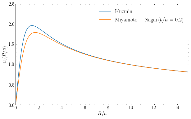
The rotation curve as a function of \(R/a\) for the Kuzmin model together with the equivalent-mass spherical model is given in the following figure
[23]:
from galpy import potential
figsize(10,6)
a= 1.
kzp= potential.KuzminDiskPotential(amp=5.,a=a)
kzp_spher= EquivalentMassSphericalPotential(amp=5.,\
                cumulmassfunc=lambda R: 1.-a/numpy.sqrt(R**2+a**2))
line_kuzmin= kzp.plotRotcurve(Rrange=[0.,15.],\
                label=r'$\mathrm{Kuzmin}$',yrange=[0.,1.75],
                xlabel=r'$R/a$',ylabel=r'$v_c(R/a)$')
line_kuzmin_spher= kzp_spher.plotRotcurve(Rrange=[0.,15.],\
                label=r'$\mathrm{Spherical\ with\ same}\ M(<R)$',
                overplot=True)
legend(handles=[line_kuzmin[0],line_kuzmin_spher[0]],
       fontsize=18.,loc='upper right',frameon=False);
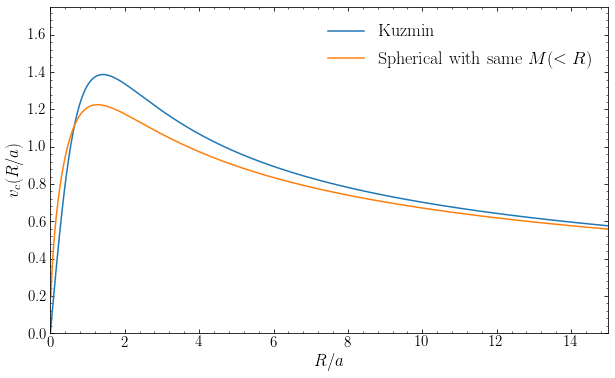
At \(R/a \ll 1\) the rotation curve of the Kuzmin disk in Equation \(\eqref{eq-vc-kuzmin}\) goes as \(v_c(R) \propto R\); this is similar to the behavior in a homogeneous-density sphere, because the surface density is constant at \(R/a \ll 1\) (see Equation \([\ref{eq-kuzmin-surfdens}]\)). At \(R/a \gg 1\), the rotation curve drops as \(v_c(R) \propto R^{-1/2}\), similar to the rotation curve of a point-mass. Because the rotation curve goes from rising linearly to falling, the rotation curve reaches a peak. From Equation \(\eqref{eq-vc-kuzmin}\) it is straightforward to compute the location of the peak, which is
These features are all obvious in the figure above. The shape of the Kuzmin rotation curve is a typical disk rotation curve for \(a \approx R_d\), the scale length of the disk. Comparing the Kuzmin rotation curve to that of the spherical mass distribution with the same enclosed-mass profile, we see that the rotation curves are quite similar even though the shape of the density distributions is completely different. This is an excellent demonstration of a general rule for disk rotation curves: they are largely set by the overall radial behavior of the mass distribution and only mildly dependent on its shape. This is why many useful insights in galactic dynamics can be obtained by approximating mass distributions as easy-to-work-with spherical distributions.
8.2.2. Thickened disk: the Miyamoto-Nagai model
The Kuzmin model provides a simple, convenient model of a razor-thin disk. But we would also like to have simple models for disks with a finite thickness. The Milky Way disk is razor-thin to a good approximation with a ratio of the scale length \(R_d\) to the scale height \(z_d\) of the mass profile of \(R_d / z_d \approx 10\), but at the next level of approximation taking into account the non-zero \(z_d\) is important, especially when looking at the properties of orbits in the disk mass distribution.
To get a thickened-disk model starting from the Kuzmin model, we can use a similar approach as that we used in Chapter 3.4: There we saw several examples of extended spherical mass distributions that were obtained by different types of smoothing of the \(\Phi(r) \propto 1/r\) behavior of the point-mass potential. The smoothing was done by replacing \(1/r\) by expressions such as \(1/\sqrt{r^2+b^2}\) (Plummer), \(1/(b+\sqrt{r^2+b^2})\) (isochrone), and \(1/(r+a)\) (Hernquist). Similarly, we can obtain a thickened Kuzmin model by replacing \(|z|\) in Equation \(\eqref{eq-kuzmin-pot}\) by \(\sqrt{z^2+b^2}\), with \(b\) a new parameter of the model, which gives the potential
Beside reducing to the razor-thin Kuzmin disk when \(b \rightarrow 0\), this potential reduces to that of a Plummer sphere when \(a\rightarrow0\), a spherical density distribution. Therefore it is clear that the ratio \(b/a\) controls how flattened the mass distribution is: \(b/a \gg 1\) gives an approximately spherical distribution with a density profile similar to that of a Plummer sphere, while \(b/a \ll 1\) corresponds to a significantly flattened distribution, with a surface-density profile similar to that of the Kuzmin model. The potential in Equation \(\eqref{eq-pot-mn}\) is a Miyamoto-Nagai potential and it remains a very popular simplified model for the gravitational potential of disks (Miyamoto & Nagai 1975).
The density corresponding to the potential in Equation \(\eqref{eq-pot-mn}\) can be computed using the Poisson equation, which gives the following complicated expression
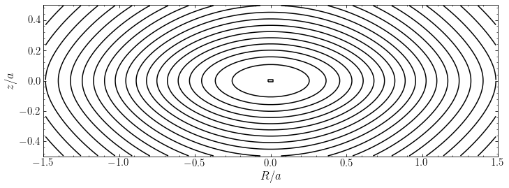
As an example of the density and potential flattening, let’s look at a Miyamoto-Nagai potential with \(b/a = 0.2\). Contours of the density in in the \((R,z)\) plane are:
[6]:
from galpy import potential
figsize(11.675,4)
mnp= potential.MiyamotoNagaiPotential(amp=10.,a=1.,b=0.2)
mnp.plotDensity(justcontours=True,rmin=-1.5,rmax=1.5,nrs=100,nzs=100)
gca().set_aspect('equal')
xlabel(r'$R/a$')
ylabel(r'$z/a$');
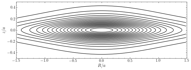
We see that the density is indeed highly flattened (the aspect ratio of this figure is such that a spherical density would appear circular). Contours of the potential are
[7]:
from galpy import potential
figsize(11.675,4)
mnp= potential.MiyamotoNagaiPotential(amp=10.,a=1.,b=0.2)
mnp.plot(justcontours=True,rmin=-1.5,rmax=1.5,nrs=100,nzs=100)
gca().set_aspect('equal')
xlabel(r'$R/a$')
ylabel(r'$z/a$');
The potential is also flattened, but much less so than the density. This is a general rule for flattened potentials: the flattening (as a deviation from sphericity) in the potential is always much smaller than that in the density. The Kuzmin model above provides another extreme example of this. There the density is contained in an infinitely thin disk, while the potential is extended in \(z\).
The radial behavior of the Miyamoto-Nagai density in Equation \(\eqref{eq-dens-mn}\) is quite different from that observed for galactic disks, which as we saw in Chapter 2.2.1 is approximately exponential \(\rho(R,z=0) \propto e^{-R/R_d}\). At \(z=0\), the density in Equation \(\eqref{eq-dens-mn}\) behaves as \(R^{-3}\) for \(R \gg a\) and the large-radius density fall-off is therefore simply a power-law of \(R\) rather than exponential. This means in particular that the density of the Miyamoto-Nagai model remains too high at large radii (e.g., at \(R \gg 15\,\mathrm{kpc}\) for the Milky Way) compared to realistic models of galactic disks. However, because the model also has a large flattening (\(b/a \ll 1\)) the total mass at large radii in the disk component at large radii is still much smaller than that in the dark halo at similar radii. Therefore, unless one is looking at orbits exactly in the mid-plane of the disk at radii much beyond the disk, the Miyamoto-Nagai model provides a reasonable model for a disk.
Because of its simplicity, the Miyamoto-Nagai model is perhaps the most often used model for a galactic disk in orbit modeling. This is because computing the gravitational potential for more realistic density distribution, such as that of an exponential disk, is significantly more complex and comes at large computational cost (as we will see below). However, it is important to keep the limitations of the Miyamoto-Nagai disk in mind when using it as an approximation for a galactic disk, in particular its problematic large \(R\) behavior.
We can compute the rotation curve for the Miyamoto-Nagai potential using Equation \(\eqref{eq-vc-midplane-general}\). Let’s compare the rotation curves of a Kuzmin potential and a Miyamoto-Nagai potential with the same mass \(M\) and the same scale length \(a\), but with a flattening \(b/a = 0.2\):
[13]:
from galpy import potential
figsize(10,6)
kzp= potential.KuzminDiskPotential(amp=10.,a=1.)
mnp= potential.MiyamotoNagaiPotential(amp=10.,a=1.,b=0.2)
line_kuzmin= kzp.plotRotcurve(Rrange=[0.,15.],\
                    label=r'$\mathrm{Kuzmin}$',yrange=[0.,2.5],
                    xlabel=r'$R/a$',ylabel=r'$v_c(R/a)$')
line_mn= mnp.plotRotcurve(Rrange=[0.,15.],\
                    label=r'$\mathrm{Miyamoto-Nagai}\,(b/a = 0.2)$',
                    overplot=True)

legend(handles=[line_kuzmin[0],line_mn[0]],
       fontsize=18.,loc='upper right',frameon=False);
We see that the rotation curve of the Miyamoto-Nagai model rises somewhat less quickly than that of the Kuzmin potential and reaches a lower peak rotation velocity at a slightly larger radius. At \(R > 2a\), the Miyamoto-Nagai rotation curve quickly approaches that of the Kuzmin model from below.
8.2.3. Models with flat rotation curves: flattened logarithmic potential
The Miyamoto-Nagai model above is a good and simple model for the potential of a galactic disk, but to represent the total mass distribution of a galaxy it needs to be combined with a bulge component and a dark-halo component. Because the Miyamoto-Nagai model itself has three parameters (mass \(M\), scale length \(a\), and scale height \(b\)) and each of the additional components require at least two parameters each (a mass and scale parameter, see the examples of spherical potentials in Section 3.4), the total number of parameters to represent a galaxy’s mass distribution becomes quite large. In general this is a good thing: the large number of parameters gives us much flexibility in the types of mass distributions that we can build from these simple building blocks. But sometimes we want to represent a galaxy with the least parameters as possible, trading flexibility in the mass model for an even simpler parameterization.
In Chapter 3.4.5 we discussed the logarithmic potential: a spherical potential \(\Phi(r) = v_c^2\, \ln r\) for which \(v_c(r) = \mathrm{constant}\). Because the logarithmic potential has a flat rotation curve, which is the rotation curve that many galaxies are observed to have, it is a simple, one-parameter (\(v_c\)) model for the total mass distribution of a galaxy. However, it is a spherical model and therefore does not form a good model for a disk galaxy with a flat rotation curve: Even when the dark-matter halo is approximately spherical, the total mass distribution that combines the halo and disk (and possible other components) will be significantly flattened for large disk galaxies. Therefore, we would like to construct a flattened version of the spherical logarithmic potential to represent the total mass distribution of disk galaxies.
A general approach to flattening any spherical potential is to replace every occurrence of \(r\) with
The parameter \(q\) is known as the flattening. This can be done either in the expression for the potential or in that of the density. However, it cannot be done in both at the same time without breaking the Poisson equation: you have to choose whether to flatten the potential or the density. The contours in the \((R,z)\) plane of a spherical potential \(\Phi(r)\) flattened to \(\Phi_\mathrm{flat}(R,z) = \Phi(m)\) through Equation \(\eqref{eq-flatten-m}\) will be ellipses with axis ratio \(q\); when the density \(\rho(r)\) is flattened to \(\rho_\mathrm{flat}(R,z) = \rho(m)\) the contours of the density are ellipses with axis ratio \(q\). It is easier to flatten the potential through Equation \(\eqref{eq-flatten-m}\) and to calculate the resulting density using the Poisson equation as \(\rho = \nabla^2 \Phi / (4\pi\,G)\) than to flatten the density and solving the Poisson equation for the potential. Therefore, flattening the potential is the more popular approach. But as always when positing a form for the potential rather than the density, this approach comes at the cost of not controlling the resulting density and having to work with whatever density comes out of \(\rho = \nabla^2 \Phi / (4\pi\,G)\).
When we apply Equation \(\eqref{eq-flatten-m}\) to the spherical logarithmic potential, we get the flattened logarithmic potential
Like the spherical logarithmic potential, this flattened version has a flat rotation curve in the mid-plane: \(v_c(R) = v_c\).
The potential contours in \((R,z)\) of a flattened logarithmic potential with \(q=0.7\) are the following
[14]:
from galpy import potential
figsize(11.675,4)
lp= potential.LogarithmicHaloPotential(amp=1.,q=0.7)
lp.plot(justcontours=True,rmin=-1.5,rmax=1.5,nrs=100,nzs=100)
gca().set_aspect('equal')
xlabel(r'$R$')
ylabel(r'$z$');
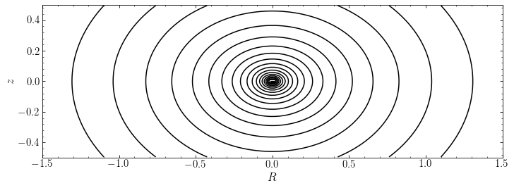
These contours appear only mildly flattened (compare, e.g., to the potential contours of the Miyamoto-Nagai model with \(b/a = 0.2\) displayed above), as would be appropriate for a disk plus a spherical dark-matter halo. However, when we look at the density corresponding to this potential, we see something funny going on
[15]:
from galpy import potential
# Code to create a colormap that plots NaN as gray, all else white
from matplotlib import cm
from matplotlib.colors import LinearSegmentedColormap
cdict1 = {'red':   ((0.0, 1.0, 1.0),
                    (1.0, 1.0, 1.0)),
         'green': ((0.0, 1.0, 1.0),
                   (1.0, 1.0, 1.0)),
         'blue':  ((0.0, 1.0, 1.0),
                   (1.0, 1.0, 1.0))}
all_white= LinearSegmentedColormap('BlueRed1', cdict1)
all_white.set_bad('0.5')
figsize(11.675,4)
p= lp.plotDensity(justcontours=False,rmin=-1.5,rmax=1.5,
                  nrs=100,nzs=100,log=True,aspect=1.)
p.set_cmap(all_white)
Rs= numpy.linspace(-0.3,0.3,101)
line, = plot(Rs,Rs/numpy.sqrt(1./0.7**2.-2.),lw=4.)
plot(Rs,-Rs/numpy.sqrt(1./0.7**2.-2.),color=line.get_color(),lw=4.)
gca().set_aspect('equal')
xlabel(r'$R$')
ylabel(r'$z$');
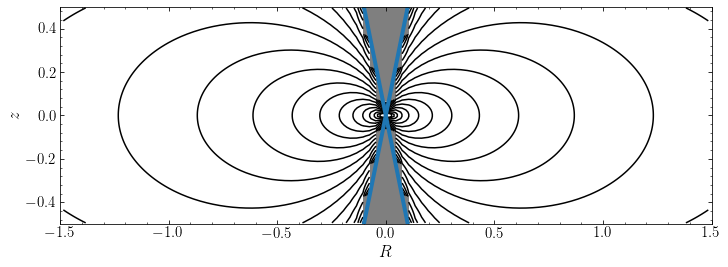
The above figure shows contours of the logarithm of the density in the \((R,z)\) plane and we have setup the colormap such that all values are white, except for where the density is negative. We see that there is a large vertical region around \(R \approx 0\) where the density is negative; this region is bounded by the blue curves (see below). In the positive-density region, the density is indeed flattened, although it has a somewhat odd dumbbell shape (compare again to the Miyamoto-Nagai density contours displayed above).
We see that even with a mild flattening of \(q=0.7\), the flattened logarithmic potential defined in Equation \(\eqref{eq-pot-flatlog}\) has regions with negative density. In those regions, the potential can therefore not be considered a physical model. This is not to say that the model with \(q=0.7\) is completely useless: as long as we stay far away from the negative density region, the potential can still provide a reasonable model galactic model.
Let’s take a closer look at the density for the flattened logarithmic potential. The density is given by
This density is negative when \(R^2 < z^2\,(1/q^2-2)\). When \(q \geq 1/\sqrt{2}\) we have that \((1/q^2-2) \leq 0\) and the density is nowhere negative. When \(q < 1/\sqrt{2}\) the density is negative in regions with \(z^2 > R^2/(1/q^2-2)\); this includes the entire \(z\) range at \(R=0\) and is bounded by the curves \(z = \pm R/\sqrt{1/q^2-2}\). These curves are displayed as the blue lines in the plot of the density above.
If we approximate the density contours in \((R,z)\) with ellipses (clearly not the greatest approximation if one looks at the density contours above), the axis ratio of these ellipses is \(q_\rho\) with
For mildly flattened distributions, we have \(1-q \approx (1-q_\rho)/3\). That is, the deviation from sphericity in the density is about three times larger than that in the potential. This is a useful rule of thumb to relate the flattening in the density and that in the potential for any potential, but don’t expect exact results from this, deviations from this particular rule can be tens of percent!
8.3. Gravitational potentials from disk density distributions
So far we have discussed models for disk density distribution that derive from simple models of the potential. While we have been successful in obtaining some simple models that can be used as a rough approximation to the mass distribution of a disk, all of the models discussed above have some issues. The density of the Miyamoto-Nagai potential falls of much slower than that of the exponential disks that we observe. The flattened logarithmic potential that can describe the overall potential of a disk plus halo system has signficant regions with negative densities as soon as the flattening becomes more than mild and can therefore not be a physically realistic model. When we flatten the density instead of the potential (e.g., using Equation \([\ref{eq-flatten-m}]\)) we avoid the issue of negative densities, but this comes at the cost of having to solve the Poisson equation for flattened densities. We will tackle that problem in this section for highly flattened systems and come back to this problem for mildly flattened systems in Chapter 13.
8.3.1. Some general considerations
We start with some general considerations about solving for the potential for a highly flattened density, which we will represent as \(\rho(R,\phi,z) = \Sigma(R,\phi|z)\,\zeta(z)\), with \(\Sigma(R,\phi|z)\) the surface density of a layer at height \(z\) and \(\zeta(z)\) defined such that \(\int \mathrm{d}z\,\zeta(z) = 1\). For such a density, the Poisson equation is best written down in cylindrical coordinates. Using the expression for the Laplacian in cylindrical coordinates in Equation (A.24) the Poisson equation becomes
To make headway in solving this equation, we introduce the Fourier transform \(f_m(\phi)\) over \(\phi\) of a function \(f(\phi)\)
with the inverse transformation given by
Taking the Fourier transform over \(\phi\) of Equation \(\eqref{eq-poisson-cylindrical}\) leads to
where every function with subscript \(m\) is defined by Equation \(\eqref{eq-fourier-phi}\). Expanding out the first term and multiplying both sides with \(R^2\) gives
Compare this equation to the differential equation that defines Bessel functions of the first kind \(J_m(x)\) (Equation B.11), which we can re-write as
The left-hand side of this equation is equal to the first three terms in Equation \(\eqref{eq-poisson-cylindrical-intermed1}\). Therefore, we can expect that solutions to Equation \(\eqref{eq-poisson-cylindrical-m}\) will be given as a sum over terms of the form \(\tilde{\Phi}_m(k,z)\,J_m(k\,R)\), because for such a form, the left-hand side of Equation \(\eqref{eq-poisson-cylindrical-intermed1}\) becomes that of an ordinary differential equation
We will continue with this solution in Section 8.3.5, where we will see that \(\tilde{\Phi}_m(k,z)\) is the Hankel transform of order \(m\) and we can solve the above equation in terms of the Hankel transform of \(\Sigma_m(R|z)\,\zeta(z)\). But we will first consider the easier case of an axisymmetric, razor-thin disk and generalize this to a finite-thickness disk before coming back to the general solution.
8.3.2. Potentials for razor-thin disks
As we already discussed in section 8.2.1 on the Kuzmin disk above, a razor-thin disk, is a disk with density \(\rho(R,\phi,z) = \Sigma(R,\phi)\,\delta(z)\). Such a disk is characterized by its surface density \(\Sigma(R,\phi)\). We start by considering an axisymmetric razor-thin disk and follow the approach introduced by Toomre (1963) for determining the potential of a disk with surface density \(\Sigma(R)\).
The approach we follow is this. Based on the considerations above, we guess a class of potential–density pairs for razor-thin disks. Then it will turn out that the set of densities forms a complete basis for all smooth \(\Sigma(R)\) mass distributions and that there is a simple way of decomposing any \(\Sigma(R)\) into a sum over the density basis functions. The potential is then obtained as the same sum over the set of potentials corresponding to the density basis functions.
For an axisymmetric disk only the \(m=0\) component of Equation \(\eqref{eq-poisson-cylindrical-m}\) is non-trivial and we have that \(\Sigma_0(R) = \Sigma(R)\) and therefore \(\Phi_0(R,z) = \Phi(R,z)\). For a razor-thin disk, this equation becomes
It is easy to check that the function
with \(k\) some constant is a solution of this equation [keeping in mind the definition of the Bessel function of the first kind in Equation \([\ref{eq-bessel-def}]\), that \(\mathrm{d}\, |z| / \mathrm{d} \,z = \mathrm{sign}(z)\), and that \(\mathrm{d} \,\mathrm{sign}(z) / \mathrm{d}\, z = 2\,\delta(z)\)], with the corresponding \(\tilde{\Sigma}(R;k)\) given by (e.g., Equation \([\ref{eq-razorthin-potderiv-surfdens}]\))
Therefore, if we can write the surface density \(\Sigma(R)\) of a razor-thin disk that we are interested in as a sum over contributions \(S_0(k)\,\tilde{\Sigma}(R;k)\) with amplitudes \(S_0(k)\), then the potential is the sum over contributions \(S_0(k)\,\tilde{\Phi}(R;k)\), because of the linearity of the Poisson equation. Thus, we write
where we can determine the \(S_0(k)\) as
because of the Fourier-Bessel theorem (Equation B.16). \(S_0(k)\) is the zero-th order Hankel transform of \(\Sigma(R)\). The gravitational potential is then given by
Equation \(\eqref{eq-pot-razorthin}\) is the general solution for the potential of a razor-thin, axisymmetric disk. The gravitational potential in the \(z=0\) mid-plane is
The circular velocity in the mid-plane can be obtained from this, noting that \(\mathrm{d}\,J_0(t)/\mathrm{d}\,t = -J_1(t)\) (Equation B.14)
When we use the expressions above to compute the potential, rotation curve, and radial and vertical forces for a given surface density profile with numerical integration, care must be taken because the Bessel functions are highly oscillatory. In the next section we consider examples where we can do all integrals analytically, and so we do not have to worry about this issue. The form of the integral for the gravitational potential in Equation \eqref{eq-pot-razorthin} is that of the Laplace transformation of \(J_0(kR)\,S_0(k)\), so razor-thin disk surface densities for which the potential has a closed form are those with known Laplace transformations.
Before continuing with a few examples, let’s consider the limit \(R,z \rightarrow \infty\) for a razor-thin mass distribution with a finite mass \(M\). Physically, we expect that the potential \(\Phi(R,z)\) should approach that of a point-mass with mass \(M\), because at distances \(r \gg\) the scale of the disk, the details of how the mass \(M\) is distributed should not matter. We can write Equation \(\eqref{eq-pot-razorthin}\) using that \(\mathrm{d} M(<R') = 2\pi\,R'\Sigma(R')\,\mathrm{d}R'\) and using integration by parts as
because \(M(0) = 0\) and \(M\,J_0(\infty) = 0\). Re-arranging this and using \(J_1(kR')\,k = -\mathrm{d} J_0(kR') / \mathrm{d}\,R'\) we find that
To solve the integral in square brackets, we need the Laplace transformation of a product of two Bessel functions of the first kind of order zero and the result is (e.g., Kausel & Irfan Baig 2012)
where \(K(m)\) is the complete elliptic integral of the first kind (see Equation B.34). At large distances, we can assume that \(M(<R') = M\) at all \(R'\) that contribute significantly to the integral in Equation \(\eqref{eq-razorthin-larger-deriv0}\) and we can then use the fundamental theorem of calculus to obtain the potential at large distances
Because \(K(0) = \pi/2\). Thus, we find that at large distances from a finite-mass, razor-thin mass distribution the potential approaches that of a point-mass of the same mass. In particular, this means that the rotation curve of any finite-mass disk will tend to the Keplerian behavior \(v_c(R) \propto R^{-1/2}\) at large distances.
8.3.3. Examples of razor-thin disks
8.3.3.1. The Mestel disk
The simplest example of using Equation \(\eqref{eq-pot-razorthin}\) is for the Mestel disk (Mestel 1963). This is the razor-thin disk with surface density
For this surface density, \(S_0(k)\) is easily computed using Equation \(\eqref{eq-hankel-surfdens-0}\)
because \(\int_0^\infty\mathrm{d} t\,J_m(t) = 1\) for all \(m\). The gravitational potential is then given by Equation \(\eqref{eq-pot-razorthin}\)
(the integral can be solved by noting that the derivative of the integral with respect to \(|z|\) is \(v_c^2\,\int_0^\infty\mathrm{d}k\,e^{-k|z|}\,J_0(kR) = 1/\sqrt{R^2+|z|^2}\) by Equation B.17). The circular velocity in the mid-plane from Equation \(\eqref{eq-vc-razorthin}\) is given by
which is simply constant (again using that \(\int_0^\infty\mathrm{d} t\,J_m(t) = 1\) for all \(m\)).
The Mestel disk therefore has a flat rotation curve and can be considered the infinitely thin limit of the flattened logarithmic potential, which also has a flat rotation curve. It is interesting to write the rotation curve \(v_c(R)\) in terms of the mass contained within \(R\) for the Mestel disk. The mass is given by
and therefore
This is the same relation between \(v_c(R)\) and \(M(<R)\) as that that holds for any spherical potential. As we discussed at the beginning of this chapter, for general disk mass distributions the mass outside of \(R\) affects the rotation curve inside of \(R\), but this is not the case for the Mestel disk!
8.3.3.2. The razor-thin exponential disk
As we discussed in Chapter 2.2.1, the surface density profiles of disk galaxies are exponential with
which we will also find convenient to write as \(\Sigma(R) = \Sigma(0)\,e^{-\alpha R}\) below (we write the central surface density as \(\Sigma(0)\) to avoid confusion with \(\Sigma_0\), the \(m=0\) component of the surface density). For future reference, we compute the enclosed mass \(M(<R)\)
For a razor-thin exponential disk, we can compute \(S_0(k)\) using Equation \(\eqref{eq-hankel-surfdens-0}\)
using a trick introduced by Kuijken & Gilmore (1989c) and again using Equation (B.17). We could work out the derivative with respect to \(\alpha\), but will find it convenient to keep it. Using this result, we can compute the potential in the mid-plane using Equation \(\eqref{eq-pot-razorthin-midplane}\)
where \(I_m(\cdot)\) and \(K_m(\cdot)\) are the modified Bessel functions of the first and second kind, respectively, defined in Equation (B.19). We have also used that \(\mathrm{d}\,I_0(x) / \mathrm{d}\,x = I_1(x)\) and \(\mathrm{d}\,K_0(x) / \mathrm{d}\,x = -K_1(x)\) (Equations B.21 and B.22). The rotation curve is then most easily computed as the derivative of this expression for \(\Phi(R,0)\) (using that \(\mathrm{d}\,I_1(x) / \mathrm{d}\,x = I_0(x)-I_1(x)/x\) and \(\mathrm{d}\,K_1(x) / \mathrm{d}\,x = -K_0(x)-K_1(x)/x\); Equations B.23 and B.24)
a result first derived by Freeman (1970). Thus, we see that using the formalism introduced in the previous section, we have been able to analytically compute the rotation curve for a realistic disk surface density. That’s pretty good!
Before showing the rotation curve of the razor-thin exponential disk, we can compute where it reaches a maximum, by finding \(\mathrm{d}\,v_c^2(R) / \mathrm{d}\,R = 0\). The derivative of \(v_c^2(R)\) is
This is a rather complicated looking function. Let’s plot it as a function of \(R/R_d\), dropping the prefactor \(\pi\,G\,\Sigma(0)\)
[18]:
from scipy import special
xs= numpy.linspace(0.,5.,101)
def dvc2dr(x):
    return 2*x*special.i0(x/2.)*special.k0(x/2.)\
         -x**2.*(special.i0(x/2.)*special.k1(x/2.)
                  -special.i1(x/2.)*special.k0(x/2.))
plot(xs,dvc2dr(xs))
xlabel(r'$R/R_d$')
ylabel(r'$\mathrm{d}\,v_c^2(R) / \mathrm{d}\,R$');
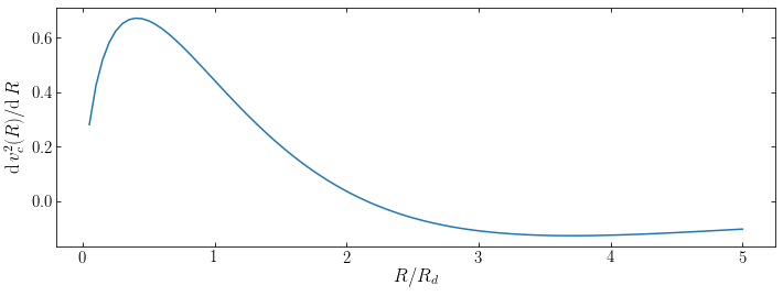
The derivative becomes zero somewhere in the range \(2 < R/R_d < 3\). We cannot solve for this zero crossing analytically, but let’s find it numerically
[19]:
from scipy import optimize
opt= optimize.brentq(dvc2dr,2.,3.)
print("The exponential-disk rotation curve peaks at R/R_d = %.3f" % opt)
The exponential-disk rotation curve peaks at R/R_d = 2.150
Thus, we find the classical result that the rotation curve of a razor-thin exponential disk peaks at \(R \approx 2.15\,R_d\).
Let’s now compare the rotation curve for the razor-thin exponential disk to that of the razor-thin Kuzmin disk with the same total mass and with scale length \(a\) such that the rotation curves peak at the same radius. Remember that the rotation curve of a Kuzmin disk peaks at \(R = \sqrt{2}\,a\).
[20]:
from galpy import potential
figsize(10,6)
kzp= potential.KuzminDiskPotential(amp=10.,a=2.15/numpy.sqrt(2.))
rp= potential.RazorThinExponentialDiskPotential(amp=10./(2.*numpy.pi),hr=1.)
line_rp= rp.plotRotcurve(Rrange=[0.,15.],\
                    label=r'$\mathrm{Exponential}$',yrange=[0.,2.5],
                    xlabel=r'$R/R_d$',ylabel=r'$v_c(R/R_d)$')
line_kuzmin= kzp.plotRotcurve(Rrange=[0.,15.],\
                    label=r'$\mathrm{Kuzmin}$',
                    overplot=True)
legend(handles=[line_rp[0],line_kuzmin[0]],
       fontsize=18.,loc='upper right',frameon=False);
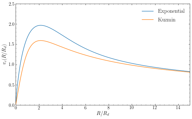
For the same mass and peak radius, the exponential disk has a higher maximum circular velocity than the Kuzmin disk. Indeed, the circular velocity for the exponential disk is larger than that for the equivalent Kuzmin disk at all radii. This is essentially because the exponential disk is more centrally concentrated than the Kuzmin disk.
We can also compare the rotation curve of the razor-thin exponential disk to that of the spherical mass distribution with the same enclosed mass, in this case given by Equation \(\eqref{eq-razorexp-encmass}\). Using the EquivalentMassSphericalPotential galpy potential class that we defined above we get
[21]:
from galpy import potential
figsize(10,6)
Rd= 1.
rp= potential.RazorThinExponentialDiskPotential(amp=10./(2.*numpy.pi),hr=Rd)
rp_spher= EquivalentMassSphericalPotential(amp=10.,\
                cumulmassfunc=lambda R: Rd**2.-Rd*(R+Rd)*numpy.exp(-R/Rd))
line_rp= rp.plotRotcurve(Rrange=[0.,15.],\
                    label=r'$\mathrm{Exponential}$',yrange=[0.,2.5],
                    xlabel=r'$R/R_d$',ylabel=r'$v_c(R/R_d)$')
line_rp_spher= rp_spher.plotRotcurve(Rrange=[0.,15.],\
                    label=r'$\mathrm{Spherical\ with\ same}\ M(<R)$',
                    overplot=True)
legend(handles=[line_rp[0],line_rp_spher[0]],
       fontsize=18.,loc='upper right',frameon=False);
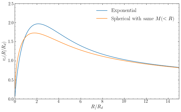
We see that the razor-thin exponential disk’s rotation curve rises to a higher peak rotation velocity and then approaches the rotation curve of the equivalent-mass spherical distribution slowly from above. As for the Kuzmin disk above, we see that the rotation curve of this disk mass distribution is only slightly different from that of the equivalent-mass spherical distribution, with the main difference being that the disky density gives a somewhat elevated circular velocity for the same radial profile.
8.3.3.3. A thin ring … and any razor-thin disk
Now that we are well warmed up in our use of Bessel functions and elliptic integrals, we can tackle the problem of computing the gravitational potential of a thin ring that we showed earlier in this chapter to demonstrate the essential differences between spherical and flattened potentials. We’ll consider an infinitely thin, axisymmetric ring of radius \(a\) with density
Therefore, the surface density is \(\Sigma(R) = M\,\delta(R-a)/(2\pi a)\). The parameter \(M\) is the total mass of the ring, as can be readily shown by integrating the surface density over all \((R,\phi)\). Using Equation \eqref{eq-hankel-surfdens-0}, we can compute the function \(S_0(k)\)
So far so good. The next step is where things get more complicated. Using Equation \eqref{eq-pot-razorthin}, we can compute the potential
To solve this integral, we again need the Laplace transformation of a product of two Bessel functions of the first kind of order zero and the result is (e.g., Kausel & Irfan Baig 2012)
where \(K(m)\) is again the complete elliptic integral of the first kind (see Equation B.34). Using the expression for the derivative of \(K(m)\) (Equation B.37), we can determine the forces for this potential. Taking the limit where \(R, z \gg a\), we again see that \(\Phi(R,z) \rightarrow -GM/r\), the potential of a point-mass (because \(K(0) = \pi/2\)).
Because we can decompose any razor-thin axisymmetric disk as an infinite collection of thin rings with infinitesimal masses \(\delta M(a)\) at radii \(a\) as
or
Substituting \(\delta M(a)\) for \(M\) in Equation \eqref{eq-thinring-pot} and integrating over \(a\) then gives the potential of any razor-thin surface density
Another way of obtaining this result is by swapping the order of integration in Equation \eqref{eq-pot-razorthin} and using the integral that we used in going from Equation \eqref{eq-thinring-almostpot} to Equation \eqref{eq-thinring-pot}.
8.3.4. Potentials for disks with finite thickness
So far we have discussed solving the Poisson equation to obtain the gravitational potential and rotation curves for razor-thin disks. But real disks are not razor-thin: their aspect ratios \(R_d/z_d\) are \(\approx10\) and the thickness of the disk has a significant effect on the orbits of stars in the disk. This will become clearer when we discuss orbits in disk mass distributions in Chapter 10.
To compute the potential for a disk with finite thickness, we can treat each layer as a razor-thin disk, obtain the contribution to the gravitational potential from each layer using Equation \(\eqref{eq-pot-razorthin}\), and then add all of these contributions together to compute the total potential. In general this is cumbersome, because the \(S_0(k)\) factor in the integral for the potential will depend on the height of each layer. Fortunately, observations of disks demonstrate that the thickness is roughly independent of radius and therefore to a good approximation we can approximate the density of galactic disks as
where we define \(\zeta(z)\) such that \(\int \mathrm{d}z\,\zeta(z) = 1\), such that \(\Sigma(R,\phi)\) is the surface density. If the disk is axisymmetric, this becomes \(\rho(R,z) = \Sigma(R)\,\zeta(z)\). For such a density distribution, the surface density of a layer at \(z=z'\) is given by \(\Sigma(R)\,\zeta(z')\,\mathrm{d}z\). When we only consider this layer, \(\zeta(z')\) is a constant and the potential \(\mathrm{d}\Phi(R,z)\) of this layer at \((R,z)\) is then given by Equation \(\eqref{eq-pot-razorthin}\)
The total potential is therefore given by
and the radial and vertical component of the force are
8.3.4.1. The double-exponential disk
As an example of a disk with a finite thickness, let’s look at a finite-thickness version of the razor-thin exponential disk that we discussed above. We thicken the disk by replacing the \(\delta(z)\) vertical profile by an exponential
where we \(z_d = 1/\beta\) is the scale height. Because of the two exponentials, this disk is known as the double-exponential disk. It is a very popular model for disk galaxies.
Computing the gravitational potential and forces of the double-exponential disk can be done through the equations given in the previous subsection. These can be somewhat simplified, as described in Appendix A of Kuijken & Gilmore (1989c). We won’t go into that level of detail here. Instead, we will gain some analytical insight on the dependence of the rotation curve on the thickness of the disk.
To compute the rotation curve of the double-exponential disk, we first compute \(\Phi(R,0)\). Equation \(\eqref{eq-pot-thickdisk}\) applied with \(\zeta(z') = \beta\,e^{-\beta|z|}/2\) gives
where \(S_0(k)\) is given by Equation \(\eqref{eq-S0-razorthinexp}\). This is a tough integral to solve! In the limit of a thin disk, \(\beta \gg 1\) and we can approximate \(1/(\beta+k) \approx (1-k/\beta)/\beta\). Note that the approximation we are making is not entirely warranted: the integral extends over all \(k\), but we require \(k/\beta \ll 1\) for this to be a good approximation. However, for large \(k\), \(S_0(k) \propto 1/k\) and the amplitude of the oscillatory \(J_0(kR) \propto 1/\sqrt{k}\), so contributions to the integral at high \(k\) are small. In this approximation we have that
where to go to the second line we have substituted the razor-thin potential for the first term and to go to the third line we have used Equation \(\eqref{eq-invhankel-surfdens-0}\). The circular velocity curve is then approximately
where we have used that \(\mathrm{d}\,\Sigma(R) / \mathrm{d}\,R = -\Sigma(R)/R_d\) for the exponential disk. Thus, we see that a thickened exponential disk has a lower circular velocity than the razor-thin disk with the same surface-density profile; the difference in \(v_c^2(R)\) is proportional to the aspect ratio \(z_d/R_d\) of the disk and proportional to \(R\,e^{-R/R_d}\). To get a better sense of the magnitude of the difference, we use that \(v_{c,\mathrm{razor-thin}}^2(R) \approx 2\,\pi\,G\,\Sigma(0)\,R/5\) up to a numerical factor close to 1 at \(R\approx 2R_d\) (near the peak of the rotation curve) and therefore the relative difference in the rotation curve is
Thus, we see that the rotation curve is only affected by \(\lesssim 10\,\%\) for thick, exponential disks compared to the razor-thin case. The disk thickness causes the rotation curve to be lower than that for a razor-thin disk: very flattened mass is able to sustain a higher rotation velocity than less flattened mass.
The following figure compares the rotation curve for the double-exponential disk with \(z_d/R_d = 0.2\), numerically computed using galpy, to that of the razor-thin disk and to the approximation in Equation \(\eqref{eq-vc-dblexp-approx}\):
[22]:
from galpy import potential
from matplotlib.ticker import FuncFormatter
figsize(10,6)
# The way galpy is currently written, it does not properly compute
# v_c for the double-exp disk at R > 5, so need to use a smaller Rd
# to go all the way to R=15 Rd
Rd= 0.2
zd= 0.2*0.2
rp= potential.RazorThinExponentialDiskPotential(amp=10.,hr=Rd)
dp= potential.DoubleExponentialDiskPotential(amp=10./2./zd,hr=Rd,hz=zd)
line_rp= rp.plotRotcurve(Rrange=[0.,3.],\
                    label=r'$\mathrm{Razor-thin\ exponential}$',
                    yrange=[0.,2.5],
                    xlabel=r'$R/R_d$',ylabel=r'$v_c(R/R_d)$')
line_dp= dp.plotRotcurve(Rrange=[0.,3.],\
                    label=r'$\mathrm{Double\ exponential}\,(z_d/R_d = 0.2)$',
                    overplot=True)
# Also compute the approximation above
Rs= numpy.linspace(0.,3.,1001)
line_approx= plot(Rs,numpy.sqrt(numpy.pi*rp._amp*Rs**2./Rd\
                  *(special.i0(Rs/2./Rd)*special.k0(Rs/2/Rd)
                      -special.i1(Rs/2/Rd)*special.k1(Rs/2./Rd))\
                    -2*numpy.pi*rp._amp*Rs*zd/Rd*numpy.exp(-Rs/Rd)),
                 label=r'$\mathrm{Approximation}$',ls='--')
# To get the ticklabels correct, need to multiply the labels
def perRd(x,pos):
    return r'$%.0f$' % (x*5.)
gca().xaxis.set_major_formatter(FuncFormatter(perRd))
legend(handles=[line_rp[0],line_dp[0],line_approx[0]],
       fontsize=18.,loc='upper right',frameon=False);
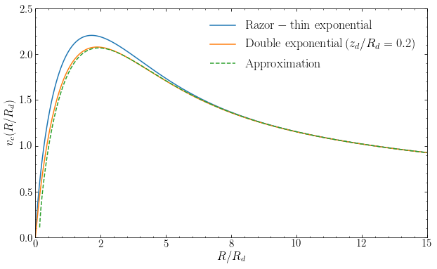
We see that the approximation does an excellent job of correcting the razor-thin rotation curve for the effect of disk thickness.
8.3.5. Gravitational potentials for non-axisymmetric density distributions
We are now ready to discuss the general solution of the Poisson equation for a disky, non-axisymmetric mass distribution. For simplicity, we will assume that the vertical and planar parts of the density separate as \(\rho(R,\phi,z) = \Sigma(R,\phi)\,\zeta(z)\), but everything we derive is easy to generalize to the general case: the Fourier and Hankel transforms of \(\Sigma(R,\phi)\) that we perform to obtain a solution would depend on \(z\) in the general case, but otherwise all expressions would be the same.
As discussed in Section 8.3.1, we start by taking the Fourier transform over \(\phi\), to get the Poisson equation for \(\Phi_m(R,z)\) (Equation \([\ref{eq-poisson-cylindrical-m}]\), which we repeat here for the case where the density separates)
Similar to what we did in Section 8.3.2, we can then easily check using the definition of the Bessel functions that the function
is a solution of the Poisson equation, with surface density
Just like for the axisymmetric case, if we can write the target surface density \(\Sigma_m(R)\) as a sum over contributions \(S_m(k)\,\tilde{\Sigma}_m(R;k)\) with amplitudes \(S_m(k)\), then the potential is the sum over contributions \(S_m(k)\,\tilde{\Phi}_m(R;k)\), because of the linearity of the Poisson equation. Thus, we write
where we can determine the \(S_m(k)\) as
because of the Fourier-Bessel theorem (Equation B.16). \(S_m(k)\) is the m-th order Hankel transform of \(\Sigma_m(R)\). Like for the thick, axisymmetric disks in Equation \(\eqref{eq-pot-thickdisk}\), we obtain the total gravitational potential \(\Phi_m(R,z)\) by combining the contributions from all of the different layers and then use the inverse Fourier transform (Equation \([\ref{eq-fourier-phi-inv}]\)) to get \(\Phi(R,\phi,z)\). After all is said and done we arrive at
Equation \(\eqref{eq-pot-disk-general}\) is the general solution for the potential of a disk. This is clearly a complicated expression: the solution involves a quadruple integral and an infinite sum over \(m\). It is therefore best to think of this as a formal full solution that can be usefully applied in cases of higher symmetry, such as those that we discussed above. For example, it can be used to get the potential for a razor-thin, non-axisymmetric disk with \(\zeta(z) = \delta(z)\) and a simple Fourier transform in \(\phi\) (e.g., an elliptical disk which only has non-zero \(\Sigma_m\) for \(m=0\) and \(m=2\)).